Fast Derandomized Low-rank Approximation and Extensions Thanks: The results of this paper have been presented at the Eleventh International Computer Science Symposium in Russia (CSR’2016), in St. Petersbourg, Russia, June 2016 (see [PZ16]).
Abstract
- •
Low-rank approximation of a matrix by means of structured random sampling has been consistently efficient in its extensive empirical studies around the globe, but adequate formal support for this empirical phenomenon has been missing so far.
- •
Based on our novel insight into the subject, we provide such an elusive formal support and derandomize and simplify the known numerical algorithms for low-rank approximation and related computations.
- •
Our techniques can be applied to some other areas of fundamental matrix computations, in particular to the Least Squares Regression, Gaussian elimination with no pivoting and block Gaussian elimination.
- •
Our formal results and our numerical tests are in good accordance with each other.
Key Words:
Low-rank approximation, Random sampling, Derandomization
2000 Math. Subject Classification:
15A52, 68W20, 65F30, 65F20
1 Introduction
1.1 The problem of low-rank approximation and our progress briefly
Low-rank approximation of a matrix has a variety of applications to the most fundamental matrix computations [HMT11] and numerous problems of data mining and analysis, “ranging from term document data to DNA SNP data” [M11]. Classical solution algorithms use SVD or rank-revealing factorizations, but the alternative solution by means of random sampling is numerically reliable, robust, and computationally and conceptually simple and has become highly and increasingly popular in the last decade (see [HMT11], [M11], and [GL13, Section 10.4.5] for surveys and ample bibliography).
In particular the paper [HMT11] proves that random sampling algorithms applied with Gaussian multipliers produce low-rank approximation with a probability close to 1, but empirically the algorithms work as efficiently with various random structured multipliers.
Adequate formal support for this empirical evidence has been elusive so far, but based on our new insight we obtain such a support and furthermore derandomize these algorithms and simplify them by applying them with some sparse and structured multipliers. The known links enable immediate extensions of our results to various important computations in numerical linear algebra and data mining and analysis, but we also extend them to other fundamental computational problems solved by using random multipliers. We outline our results in this section. They are in good accordance with our numerical tests of Section 5.
1.2 Some definitions
- •
Typically we use the concepts “large”, “small”, “near”, “close”, “approximate”, “ill-conditioned” and “well-conditioned” quantified in the context, but we specify them quantitatively as needed.
- •
Hereafter “” means “much less than”; “flop” stands for “floating point arithmetic operation”.
- •
is the identity matrix. is a matrix filled with zeros. is a vector filled with zeros.
- •
denotes a block matrix with the blocks .
- •
denotes a block diagonal matrix with diagonal blocks .
- •
, , and denote the rank, numerical rank, and the spectral norm of a matrix , respectively.
- •
and , and denote its transpose and Hermitian transpose, respectively.
- •
An matrix is called unitary if or if . If this matrix is known to be real, then it is also and preferably called orthogonal.
( and if the matrix is unitary.)
- •
is compact SVD of a matrix of rank with and denoting the unitary matrices of its singular vectors and the diagonal matrix of its singular values in non-increasing order, . ()
- •
denotes the condition number of a matrix . A matrix is called ill-conditioned if its condition number is large in context and is called well-conditioned if this number is reasonably bounded.
(An matrix is ill-conditioned if and only if it has a matrix of a smaller rank nearby or equivalently if and only if its rank exceeds its numerical rank; an matrix is well-conditioned if and only if it has full numerical rank . A matrix is unitary if and only if .)
- •
“Likely” means “with a probability close to 1”, the acronym “i.i.d.” stands for “independent identically distributed”, and we refer to “standard Gaussian random” variables just as “Gaussian”.
- •
We call an matrix Gaussian and denote it if all its entries are i.i.d. Gaussian variables.
- •
, , and denote the classes of Gaussian, real, or complex matrices, respectively.
- •
, , and , for , denote the classes of matrices (of rank at most ) where both matrix and matrix are Gaussian, real, and complex, respectively.
- •
If and , then we call an factor-Gaussian matrix of expected rank . (In this case the matrices , and have rank with probability 1 by virtue of Theorem A.1.)
1.3 The basic algorithm
A matrix can be represented (respectively, approximated) by a product of two matrices and if and only if (respectively, ), and our main goal is the computation of such a representation or approximation.
We begin with the following basic algorithm for the fixed rank problem, where the integer or is known. Otherwise we can compute it by means of binary search based on recursive application of the algorithm or proceed, e.g., as in our Algorithm 1.2 of Section 1.5.
Algorithm 1.1.
Range Finder (See Figure 1 and compare [HMT11, Algorithms 4.1 and 4.2]).
- Input:
-
An matrix , a nonnegative tolerance , and an integer such that .
- Initialization:
-
Fix an integer such that . Generate an matrix .
- Computations:
-
- 1.
Compute the matrix . Remove its columns that have small norms.
- 2.
Orthogonalize its remaining columns (cf. [GL13, Theorem 5.2.3]), compute and output the resulting matrix where .
- 3.
Estimate the error norm for .
If , output SUCCESS; otherwise FAILURE.
- 1.
At Stage 3 probabilistic estimate for the norm can be given by the norm for a random matrix and a reasonably small positive integer (this would extend the Frievalds’ probabilistic test of [F77] (cf. [MR95], [AS00])). [HMT11, Algorithm 4.2] chooses random matrix at Stage 1 and then proceeds with and .
If Stage 3 outputs SUCCESS, then a rank- approximation to the matrix is given by the matrix ,11 1 By applying rank-revealing orthogonalization at Stage 2 we can remove some extraneous columns and obtain rank- approximation of the matrix . but the papers [HMT11, Section 5] and [CW13] avoid costly multiplication of by . Their alternative solution relies on the extension of Stage 1 to randomized approximation of the leading part of the compact SVD of the matrix , associated with its largest singular values.
The complexity of these algorithms is dominated at Stage 1, which uses flops in the case of generic matrices and . With intricate application of sparse embedding multipliers , the paper [CW13] computes a low-rank approximation (with failure probability at most 1/5) by using about flops for generic input , but alternative computations using flops can be still of interest (see Section 1.8).
1.4 The choice of multipliers: basic observations
We readily verify the following theorem (see Section 4.3):
Theorem 1.1.
Given an matrix with and a reasonably small positive tolerance , Algorithm 1.1 outputs SUCCESS if and only if .
Definition 1.1.
For two integers and , , and any fixed multiplier , partition the set of matrices with into the set of “-good” matrices such that and the set of “-bad” matrices such that .
The following simple observations should be instructive.
Theorem 1.2.
(Cf. Remark 1.2.) Consider a vector of dimension , an unitary matrix , and an unitary matrix , so that matrix is unitary. Then
(i) , that is, the map multiplies the class of -good matrices by the unitary matrix ,
(ii) , that is, appending a column to a multiplier can only expand the class , and
(iii) this class fills the whole space or if .
Proof.
Part (i) follows because . Part (ii) follows because . Part (iii) follows because if is an unitary matrix. ∎
1.5 A recursive algorithm
Based on Theorem 1.2 we devise the following algorithm where is not known.
Algorithm 1.2.
Recursive low-rank representation/approximation of a matrix. See Figure 2 and cf. [HMT11, Algorithm 4.2].
- Input:
-
An matrix and a nonnegative tolerance .
- Computations:
-
- 1.
Generate an unitary matrix .
- 2.
Fix positive integers such that (in particular for all if ) and represent the matrix as a block vector where the block has size for .
- 3.
Recursively, for , apply Algorithm 1.1 to the matrix by substituting for and for . Stop when the algorithm outputs SUCCESS.
- 1.
By virtue of part (iii) of Theorem 1.2 the algorithm stops and outputs SUCCESS either at the th Stage (when ) or earlier, and we are surely interested in yielding SUCCESS already for and in saving flops for matrix multiplications at Stage 3.
Remark 1.1.
Remark 1.2.
Clearly, the blocks and of the unitary matrix are unitary as well, but we can readily extend both Theorem 1.2 and Algorithm 1.2 to the case where we apply them to a nonsingular and well-conditioned (rather than unitary) matrix . In that case all multipliers and all their blocks are also well-conditioned matrices of full rank, and moreover and for all and (cf. [GL13, Corollary 8.6.3]).
1.6 Benefits of using Gaussian and random structured multipliers
Theorem 1.3.
Let Algorithm 1.1 be applied with a Gaussian multiplier . Then
(i) with probability 1 if (cf. Theorem 4.1) and
(ii) it is likely that if , and the probability that approaches 1 fast as increases from (cf. Theorem 4.3).
The theorem implies that Algorithm 1.2 is likely to output SUCCESS at Stage for the smallest such that in the case where denotes a Gaussian (rather than unitary) matrix.
An matrix of subsample random Fourier or Hadamard transform22 2 Hereafter we use the acronyms SRFT and SRHT. is defined by random variables (see Remark 3.3), and we can pre-multiply it by a vector by using flops, for of order , (see [HMT11, Sections 4.6 and 11], [M11, Section 3.1], and [T11]). For comparison, an Gaussian matrix is defined by its random entries, and we need flops in order to pre-multiply it by a vector.
SRFT and SRHT multipliers are universal, like Gaussian ones: Algorithm 1.1 applied with such a multiplier is likely to approximate closely a matrix having numerical rank at most , although the estimated failure probability , for with Gaussian multipliers increases to order of in the case of SRFT and SRHT multipliers (cf. [HMT11, Theorems 10.9 and 11.1], [M11, Section 5.3.2], and [T11]).
Empirically Algorithm 1.1 with SRFT multipliers fails very rarely even for , although for some special input matrices it is likely to fail if (cf. [HMT11, Remark 11.2] or [M11, Section 5.3.2]). Researchers have consistently observed similar empirical behavior of the algorithm applied with SRHT and various other multipliers (see [HMT11], [M11], [W14], [PQY15], and the references therein),33 3 In view of part (i) of Theorem 1.2, the results cited for the classes of SRFT and SRHT matrices also hold for the products of these classes with any unitary matrix, in particular for the class of submatrices of an circulant matrix, each made up of randomly chosen columns (see Remark 3.3). but so far no adequate formal support for that empirical observation has appeared in the huge bibliography on this highly popular subject.
1.7 Our goals, our dual theorem, and its implications
In this paper we are going to
(i) fill the void in the bibliography by supplying a missing formal support for the cited observation, with far reaching implications (see parts (ii) and (iv) below),
(ii) define new more efficient policies of generation and application of multipliers for low-rank approximation,
(iii) test our policies numerically, and
(iv) extend our progress to other important areas of matrix computations.
Our Dual Theorem 1.4 below reverses the assumptions of our Primal Theorem 1.3 that a multiplier is Gaussian, while a matrix is fixed.
Theorem 1.4.
Let and
(in which case
and, with a probability close to 1,
). Furthermore let
and
. Then
(i) Algorithm 1.1
outputs a rank- representation of a matrix
with probability 1
if and if , and
(ii) it
outputs a rank- approximation of that matrix
with a probability close to 1 if
and approaching 1 fast as the integer increases from .
Proof.
See Theorem 4.4. ∎
Corollary 1.1.
Part (ii) of Theorem 1.4 implies that Algorithm 1.1 succeeds for the average input matrix that has a small numerical rank (and thus in a sense to most of such matrices) if the multiplier is any unitary matrix (or even any well-conditioned matrix of full rank) and if the average matrix is defined under the Gaussian probability distribution. The former provision, that , is natural for otherwise we could have replaced the multiplier by an matrix for some integer . The latter customary provision is natural in view of the Central Limit Theorem.
For an immediate implication of Theorem 1.4, on the average input having numerical rank at most , Algorithm 1.2 applied with any unitary or even any nonsingular and well-conditioned multiplier outputs SUCCESS at its earliest recursive Stage at which the dimension exceeds . This can be viewed as derandomization of Algorithms 1.1 and 1.2 versus their application with Gaussian sampling.
1.8 Related work, our novelties, and extension of our progress
Part (ii) of our Theorem 1.3 is implied by [HMT11, Theorem 10.8], but our specific supporting estimates are more compact, cover the case of any (whereas [HMT11] assumes that ), and we deduce them by using a shorter proof (see Remark 4.3). Our approach and our results of Section 1.7 are new, and so are our families of sparse and structured multipliers and the policies of their generation, combination, and application in Sections 2 and 3 as well.
By applying the well-known links, we can extend our results for low-rank approximation to various fundamental problems of matrix computations and data mining and analysis, but our duality techniques can be extended to other important computational problems as well. In Section 6 (Conclusions) we show such an extension to the Least Squares Regression.44 4 Hereafter we use the acronym “LSR”. Another extension in [PZa] supports numerically safe performance of Gaussian elimination with no pivoting55 5 Pivoting, that is, row or column interchange of an input matrix for avoiding numerical problems in Gaussian elimination, is communication intensive and has become the bottleneck of Gaussian elimination in the present day computer environment. Preprocessing with randomized and derandomized multipliers is a natural means for overcoming this problem (cf. [BBBDD14], [PQY15], [PZa]). and block Gaussian elimination. The extensions provide new insights and new opportunities and should motivate further effort and further progress.
Extensive decade-long work of a number of authors on an alternative approach to Low-Rank Approximation and Least Squares Regression has culminated in the paper [CW13]. Its algorithms succeed for these problems with a probability at least 4/5, whereas we only reach solution for the average input. Our study, however, leads to some benefits, which should compensate for this deficiency.
1. We show the power of a very large class of multipliers, including various sparse and structured ones. This can be interesting, e.g., for some special structured inputs (see Remark 3.2), but not only for them. Indeed, see our Remark 3.4 and compare the following excerpt from [BCDHKS14]: “The traditional metric for the efficiency of a numerical algorithm has been the number of arithmetic operations it performs. Technological trends have long been reducing the time to perform an arithmetic operation, so it is no longer the bottleneck in many algorithms; rather, communication, or moving data, is the bottleneck”.
2. In order to make the probability of failure less than , the complexity bound of [CW13] involve overhead of order , which greatly exceeds the overhead in the case of our average case estimates.
3. [CW13] studies the fixed rank problem; in the case where the input numerical rank is not known, our Algorithm 1.2 substantially decreases the computational overhead versus binary search.
4. Unlike [CW13] we cover the case where the ratio is not very large, which can still be interesting in some applications.
5. Our analysis is quite simple and conceptually distinct and should be of independent interest because it provides elusive explanation of a well-known empirical phenomenon (cf. Section 1.1).
1.9 Organization of the paper
We organize our presentation as follows:
- •
- •
In Section 3 we present some efficient sparse and structured multipliers for low-rank approximation.
- •
- •
Section 5 (the contribution of the second and the third authors) covers our numerical tests.
- •
In Section 6 we extend our approach to the LSR computations.
- •
The Appendix covers some auxiliary results for computations with random matrices.
2 Preventing and managing the unlikely failure of Algorithm 1.1
Our conflicting goals and simple recipes.
We try to decrease:
(i) the cost of the generation of a multiplier and of the computation of the matrix ,
(ii) the chances for the failure of Algorithm 1.1, and
(iii) the rank of the computed approximation of a matrix .
Towards goal (i) we propose using sparse and structured multipliers in the next section. They are pre-multiplied by a vector and by a matrix at a low cost even for .
Towards goal (ii) we can expect to succeed whenever integer parameter exceeds , but our chances for success grow fast as increases. Such an increase is in conflict with our goal (iii), but we can alleviate the problem by using the following simple technique.
Randomized Compression Algorithm (see Figure 3).
- 1.
Fix a sufficiently large dimension , which is still much smaller than , generate a sparse and structured multiplier , and compute the product (by using flops).
- 2.
Fix a smaller integer such that , generate a Gaussian multiplier , and compute and output the matrix (by using flops, dominated at Stage 1 if ).
By virtue of Theorem 1.3 this algorithm is likely to succeed, but in our extensive tests in Section 5 even the following simple heuristic recipe has always worked.
Heuristic Compression Algorithm (linear combination of failed multipliers): if the first recursive steps of Algorithm 1.2 have failed for , then apply Algorithm 1.1 with a multiplier where for all and for a fixed or random choice of the signs . (More generally, one can choose complex values on the unit circle, letting for all .)
Remark 2.1.
In our study above we rely on the results of Theorem 1.4, which cover the average input matrices. Real computations can deal with “rare special” input matrices , not covered by Theorem 1.4, but in our tests in Section 5 with a variety of inputs, our small collection of sparse and structured multipliers of the next section turned out to be powerful enough for handling various important classes of special matrices as well.
Remark 2.2.
Reusing multipliers. Recall from [HMT11, Sections 8 and 9] that for all the matrices and , for , , and , are the orthogonal projections of the matrices and , respectively, onto the range of the matrix . Hence , and so at the -th stage of Algorithm 1.2, for , we can reuse such projections computed at its Stage rather than recompute them.
3 Generation of multipliers. Counting flops and random variables
In our tests we have consistently succeeded by using multipliers from a limited family of very sparse and highly structured orthogonal matrices of classes 13–17 of Section 5.3, but in this section we also cover a greater variety of other sparse and structured matrices, which form an extended family of multipliers.
We proceed in the following order. Given two integers and , , we first generate four classes of very sparse primitive unitary matrices, then combine them into some basic families of matrices (we denote them in this section), and finally define multipliers as submatrices made up of columns, which can be fixed (e.g., leftmost) or chosen at random. The matrix is unitary if so is the matrix , and more generally (cf. [GL13, Theorem 8.6.3]).
3.1 matrices of four primitive types
- 1.
- 2.
A diagonal matrix , with fixed or random diagonal entries such that for all (and so all entries lie on the unit circle , being either nonreal or ).
- 3.
An -circular shift matrix
and its transpose for a scalar such that either or . We write , call unit down-shift matrix, and call the special permutation matrix the unit circulant matrix.
- 4.
The latter primitive matrices are very sparse, have nonzero entries evenly distributed throughout, and can be pre-multiplied by a vector by using from 0 to flops.
All our primitive matrices, except for the matrix , are unitary or real orthogonal. Hence, for the average input matrix , Algorithm 1.1 succeeds with any of their submatrix by virtue of Theorem 1.4, and similarly with any submatrix of the matrix of full rank .
For specific input matrices the algorithm can fail with some of our primitive multipliers (e.g., this is frequently the case where both input matrix and multiplier are sparse), but in the next subsections we readily combine primitives 1–4 into families of sparse and/or structured matrices, and in Section 5 we consistently and successfully test their submatrices as multipliers.
3.2 Family (i): multipliers based on the Hadamard and Fourier processes
At first we recall the following recursive definition of dense and orthogonal (up to scaling by constants) matrices of Walsh-Hadamard transform for (cf. [M11, Section 3.1] and our Remark 3.1):
| (3.1) |
for , , and the Hadamard primitive matrix of type 4 for .
For demonstration, here are the matrices and shown with their entries,
but for larger dimensions , recursive representation (3.1) enables much faster pre-multiplication of a matrix by a vector, namely it is sufficient to use additions and subtractions for .
Next we sparsify this matrix by defining it by a shorter recursive process, that is, by fixing a recursion depth , , and applying equation (3.1) where , , and for . For two positive integers and , we denote the resulting matrix and for call it –Abridged Hadamard (AH) matrix. In particular,
For a fixed , the matrix is still orthogonal up to scaling, has nonzero entries in every row and column, and hence is sparse unless is a small integer.
Then again, for larger dimensions , we can pre-multiply such a matrix by a vector much faster if, instead of the representation by its entries, we apply recursive process (3.1), which involves just additions and subtractions and allows highly efficient parallel implementation (cf. Remark 3.4).
We similarly obtain sparse matrices by shortening a recursive process of the generation of the matrix of discrete Fourier transform (DFT) at points, for :
| (3.2) |
In particular ,
The matrix is unitary up to scaling by . We can pre-multiply it by a vector by using flops, and we can efficiently parallelize this computation if, instead of representation by entries, we apply following recursive representation (cf. [P01, Section 2.3] and our Remark 3.1):66 6 This is a representation of FFT, called decimation in frequency (DIF) radix-2 representation. Transposition turns it into an alternative representation of FFT, called decimation in time (DIT) radix-2 representation.
| (3.3) |
Here is the matrix of odd/even permutations such that , , , , , ; , , and is the scalar 1.
We sparsify this matrix by defining it by a shorter recursive process, that is, by fixing a recursion depth , , replacing for by the identity matrix , and then applying equation (3.3) for , .
For and , we denote the resulting matrix and call it -Abridged Fourier (AF) matrix. It is also unitary (up to scaling), has nonzero entries in every row and column, and thus is sparse unless is a small integer. We can represent such a matrix by its entries, but then again its pre-multiplication by a vector involves just flops and allows highly efficient parallel implementation if we rely on recursive representation (3.3).
By applying fixed or random permutation and scaling to AH matrices and AF matrices , we obtain the families of –Abridged Scaled and Permuted Hadamard (ASPH) matrices, , and –Abridged Scaled and Permuted Fourier (ASPF) matrices, where and are two matrices of permutation and diagonal scaling of primitive classes 1 and 2, respectively. Likewise we define the families of ASH, ASF, APH, and APF matrices, , , , and , respectively. Each random permutation or scaling contributes up to random parameters.
Remark 3.1.
The following equations are equivalent to (3.1) and (3.3):
where denotes a Hadamard’s primitive matrix of type 4. By extending the latter recursive representation we can define matrices that involve more random parameters. Namely we can recursively incorporate random permutations and diagonal scaling as follows:
| (3.4) |
Here are random permutation matrices of primitive class 1 and are random matrices of diagonal scaling of primitive class 2, for all . Then again we define –abridged matrices and by applying only recursive steps (3.4) initiated at the primitive matrix , for .
With these recursive steps we can pre-multiply matrices and by a vector by using at most additions and subtractions and at most flops, respectively, provided that divides .
3.3 -circulant, sparse -circulant, and uniformly sparse matrices
An -circulant matrix
for the matrix of -circular shift, is defined by a scalar and by the first column and is called circulant if and skew-circulant if . Such a matrix is nonsingular with probability 1 (see Theorem A.1) and is likely to be well-conditioned [PSZ15] if and if the vector is Gaussian.
Remark 3.2.
One can compute the product of an circulant matrix with an Toeplitz or Toeplitz-like matrix by using flops (see [P01, Theorem 2.6.4 and Example 4.4.1]).
FAMILY (ii) of sparse -circulant matrices is defined by a fixed or random scalar , , and by the first column having exactly nonzero entries, for . The positions and the values of nonzeros can be randomized (and then the matrix would depend on up to random values).
Such a matrix can be pre-multiplied by a vector by using at most flops or, in the real case where and for all , by using at most additions and subtractions.
The same cost estimates apply in the case of the generalization of to a uniformly sparse matrix with exactly nonzeros entries, , in every row and in every column for . Such a matrix is the sum for fixed or random matrices and of primitive types 1 and 2, respectively.
3.4 Abridged -circulant matrices
First recall the following well-known expression for a -circulant matrix:
where , , , , and (cf. [P01, Theorem 2.6.4]). For , the expression is simplified: , , and is a circulant matrix:
| (3.5) |
Pre-multiplication of an -circulant matrix by a vector is reduced to pre-multiplication of each of the matrices and by a vector and in addition to performing flops (or flops in case of a circulant matrix). This involves flops overall and then again allows highly efficient parallel implementation.
For a fixed scalar and , we can define the matrix by any of the two vectors or . The matrix is unitary (up to scaling) if and if for all and is defined by real parameters (or by such parameters for a fixed ), which we can fix or choose at random.
Now suppose that , , and are integers, and substitute a pair of AF matrices of recursion length for two factors in the above expressions. Then the resulting abridged -circulant matrix of recursion depth is still unitary (up to scaling), defined by or parameters and , is sparse unless the positive integer is small, and can be pre-multiplied by a vector by using flops. Instead of AF matrices, we can substitute a pair of ASPF, APF, ASF, AH, ASPH, APH, or ASF matrices for the factors . All such matrices form FAMILY (iii) of –abridged -circulant matrices.
Remark 3.3.
Recall that an SRFT and SRHT matrices are the products and , respectively, where and are the matrices of (3.1) and (3.2), , are i.i.d. variables uniformly distributed on the circle , and is the submatrix formed by columns of the identity matrix chosen uniformly at random. Equation (3.5) shows that we can obtain a SRFT matrix by pre-multiplying a circulant matrix by the matrix and post-multiplying it by the above matrix .
3.5 Inverses of bidiagonal matrices
FAMILY (iv) is formed by the inverses of bidiagonal matrices
for a matrix of primitive type 2 and the down-shift matrix . In particular,
if
In order to pre-multiply a matrix by a vector , however, we do not compute its entries, but solve the linear system of equations by using flops or, in the real case, just additions and subtractions.
We can randomize the matrix by choosing up to random diagonal entries of the matrix (whose leading entry makes no impact on ).
Finally, because nonzero entries of the lower triangular matrix have absolute values 1, and clearly . Hence (the spectral condition number of ) cannot exceed for , and the same bound holds for .
3.6 Summary of estimated numbers of flops and random variables involved
Table 3.1 shows upper bounds on
(a) the numbers of random variables involved into the matrices of the four families (i)–(iv) and
(b) the numbers of flops for pre-multiplication of such a matrix by
a vector.77
7
The asterisks in the table
show that the matrices
of families (i) AF, (i) ASPF, and (iii) involve nonreal roots of unity.
For comparison, using a Gaussian multiplier involves random variables
and flops.
One can readily extend the estimates to submatrices of the matrices .
| family | (i) AH | (i) ASPH | (i) AF | (i) ASPF | (ii) | (iii) | (iv) |
| random variables | 0 | 0 | |||||
| flops complex | |||||||
| flops in real case | * | * | * |
Remark 3.4.
Other observations besides flop estimates can be decisive. E.g., a special recursive structure of an ARSPH matrix and an ARSPF matrix allows highly efficient parallel implementation of their pre-multiplication by a vector based on Application Specific Integrated Circuits (ASICs) and Field-Programmable Gate Arrays (FPGAs), incorporating Butterfly Circuits [DE].
3.7 Other basic families
There is a number of other interesting basic matrix families. According to [HMT11, Remark 4.6], “among the structured random matrices …. one of the strongest candidates involves sequences of random Givens rotations”. They are dense unitary matrices
for the DFT matrix , three random diagonal matrices , and of primitive type 2, and two chains of Givens rotations and , each of the form
for a random permutation matrix ,
Here denote random angles of rotation uniformly distributed in the range .
The DFT factor makes the resulting matrices dense, but we can sparsify them by replacing that factor by an AF, ASF, APF, or ASPF matrix having recursion depth . This would also decrease the number of flops involved in pre-multiplication of such a multiplier by a vector from order to .
We can turn Givens sequences into distinct candidate families of efficient multipliers by replacing either or both of the Givens products with sparse matrices of Householder reflections matrices of the form for fixed or random sparse vectors (cf. [GL13, Section 5.1]).
We can obtain a variety of efficient multiplier families by properly combining the matrices of basic families (i)–(iv) and the above matrices. We can use just linear combinations, but can also apply block representation as in the following real block matrix for two vectors and and a matrix of primitive class 2.
We can define new matrix families by intertwining the Hadamard and Fourier recursive steps.
4 Proof of Theorems 1.1, 1.3, and 1.4
4.1 Low-rank representation: proof
Hereafter denotes the range (column span) of a matrix .
Theorem 4.1.
(i) For an input matrix of rank , its rank- representation is given by the products provided that is an matrix such that and that is a matrix obtained by means of column orthogonalization of .
(ii) , for and an matrix , with probability if is Gaussian, and
(iii) with a probability at least if an matrix has i.i.d. random entries sampled uniformly from a finite set of cardinality .
4.2 Low-rank approximation: a basic step
Hereafter denotes the Frobenius norm of a matrix and denotes the Moore–Penrose pseudo inverse of a matrix of rank having compact SVD . (Note that .)
Lemma 4.1.
(Cf. [GL13, Theorem 2.4.8].) For an integer and an matrix where , set to 0 the singular values , for , let denote the resulting matrix, which is a closest rank- approximation of , and write Then
Theorem 4.2.
Proof.
Next apply part (i) of Theorem 4.1 for matrix replacing , recall that , and obtain
Furthermore . Therefore
Consequently, , and so (cf. Lemma 4.1)
| (4.3) |
Apply [PQY15, Corollary C.1], for and replaced by , and obtain
| (4.4) |
In our applications the value is small, and so the value is small unless the norm is large.
4.3 Proof of Theorem 1.1
If , then , . In this case is not small because , and so Algorithm 1.1 applied to with the multiplier outputs FAILURE.
4.4 Detailed estimates for primal and dual low-rank approximation
The following theorem, proven in the next subsection, bounds the approximation errors and the probability of success of Algorithm 1.1 for . Together these bounds imply part (ii) of Theorem 1.3.
Theorem 4.3.
Suppose that Algorithm 1.1 has been applied to an matrix having numerical rank and that the multiplier is an Gaussian matrix.
(i) Then the algorithm outputs an approximation of a matrix by a rank- matrix within the error norm bound such that where and and are random variables of Definition A.1.
(ii) , for and .
Remark 4.1.
Theorem 4.4.
Suppose that Algorithm 1.1, applied to a small-norm perturbation of an factor-Gaussian matrix with expected rank , uses an multiplier such that and .
(i) Then the algorithm outputs a rank- matrix that approximates the matrix within the error norm bound such that , where , , and and are random variables of Definition A.1.
(ii) , for and .
Remark 4.2.
The expected value converges to 0 as provided that . Consequently the expected value converges to the optimal value as provided that is a well-conditioned matrix of full rank and that .
Remark 4.3.
Remark 4.4.
Remark 4.5.
The Power Scheme of increasing the output accuracy of Algorithm 1.1. See [RST09], [HMST11]. Define the Power Iterations , . Then for all and [HMT11, equation (4.5)]. Therefore, at a reasonable computational cost, one can dramatically decrease the ratio and thus decrease the bounds of Theorems 4.3 and 4.4 accordingly.
4.5 Primal theorem: completion of the proof
Theorem 4.5.
For , , and of Definition A.1, it holds that
| (4.5) |
Proof.
Let be compact SVD.
By applying Lemma A.1, deduce that is a Gaussian matrix.
Denote it and obtain .
Write and let be compact SVD where is a unitary matrix.
It follows that is an unitary matrix.
Hence and are compact SVDs of the matrices and , respectively.
Therefore .
Substitute and and obtain the theorem. ∎
4.6 Dual theorem: completion of the proof
Theorem 4.6.
Suppose that , , , , and is a well-conditioned matrix of full rank such that and . Then
| (4.6) |
If in addition , that is, if is an factor-Gaussian matrix with expected rank , then
| (4.7) |
Proof.
Combine compact SVDs and and obtain . Here , , , , , , , , and are matrices of the sizes , , , , , , , , and , respectively.
Now observe that is a Gaussian matrix, by virtue of Lemma A.1 (since is a Gaussian matrix). Therefore , for .
Let denote compact SVD where and and are unitary matrices of sizes and , respectively.
Both products and are unitary matrices, and we obtain compact SVD where , , and . Therefore
Note that because and are square nonsingular diagonal matrices. Consequently
and (4.6) follows. ∎
We also need the following result implied by [S98, Corollary 1.4.19] for :
Theorem 4.7.
Suppose and are two nonsingular matrices of the same size and
Then
e.g., if .
5 Numerical Tests
Numerical experiments have been performed by Xiaodong Yan for Tables 5.2–5.4 and by John Svadlenka and Liang Zhao for the other tables. The tests have been run by using MATLAB in the Graduate Center of the City University of New York on a Dell computer with the Intel Core 2 2.50 GHz processor and 4G memory running Windows 7; in particular the standard normal distribution function randn of MATLAB has been applied in order to generate Gaussian matrices.
We calculated the -rank, i.e., the number of singular values exceeding , by applying the MATLAB function ”svd()”. We have set in Sections 5.1 and 5.2 and in Section 5.3.
5.1 Tests for inputs generated via SVD
In the tests of this subsection we generated input matrices by extending the customary recipes of [H02, Section 28.3]. Namely, we first generated matrices and by means of the orthogonalization of Gaussian matrices. Then we defined matrices by their compact SVDs, , for ; , , and . (Hence and .)
Table 5.1 shows the average output error norms over 1000 tests of Algorithm 1.1 applied to these matrices for each pair of and , , , and each of the following three groups of multipliers: 3-AH multipliers, 3-ASPH multipliers, both defined by Hadamard recursion (3.3), for , and dense multipliers having i.i.d. entries and 0, each value chosen with probability 1/3.
| 3-AH | 3-ASPH | |||
|---|---|---|---|---|
| 256 | 8 | 2.25e-08 | 2.70e-08 | 2.52e-08 |
| 256 | 32 | 5.95e-08 | 1.47e-07 | 3.19e-08 |
| 512 | 8 | 4.80e-08 | 2.22e-07 | 4.76e-08 |
| 512 | 32 | 6.22e-08 | 8.91e-08 | 6.39e-08 |
| 1024 | 8 | 5.65e-08 | 2.86e-08 | 1.25e-08 |
| 1024 | 32 | 1.94e-07 | 5.33e-08 | 4.72e-08 |
Tables 5.2–5.4 show the mean and maximal values of such an error norm in the case of (a) real Gaussian multipliers and dense real Gaussian subcirculant multipliers , for , each defined by its first column filled with either (b) i.i.d. Gaussian variables or (c) random variables . Here and hereafter in this section we assigned each random signs or with probability 0.5.
| mean | max | ||
|---|---|---|---|
| 8 | 256 | ||
| 8 | 512 | ||
| 8 | 1024 | ||
| 32 | 256 | ||
| 32 | 512 | ||
| 32 | 1024 |
| mean | max | ||
|---|---|---|---|
| 8 | 256 | ||
| 8 | 512 | ||
| 8 | 1024 | ||
| 32 | 256 | ||
| 32 | 512 | ||
| 32 | 1024 |
| mean | max | ||
|---|---|---|---|
| 8 | 256 | ||
| 8 | 512 | ||
| 8 | 1024 | ||
| 32 | 256 | ||
| 32 | 512 | ||
| 32 | 1024 |
Table 5.5 displays the average error norms in the case of multipliers of eight kinds defined below, all generated from the following Basic Sets 1, 2 and 3 of multipliers:
Basic Set 1: 3-APF multipliers defined by three Fourier recursive steps of equation (3.3), for , with no scaling, but with a random column permutation.
Basic Set 2: Sparse real circulant matrices of family (ii) of Section 3.3 (for ) having the first column vectors filled with zeros, except for ten random coordinates filled with random integers .
Basic Set 3: Sum of two scaled inverse bidiagonal matrices. We first filled the main diagonals of both matrices with the integer 101 and their first subdiagonals with . Then we multiplied each matrix by a diagonal matrix , where were random integers uniformly chosen from 0 to 3.
For multipliers we used the western (leftmost) blocks of matrices of the following classes:
- 1.
a matrix from Basic Set 1;
- 2.
a matrix from Basic Set 2;
- 3.
a matrix from Basic Set 3;
- 4.
the product of two matrices of Basic Set 1;
- 5.
the product of two matrices of Basic Set 2;
- 6.
the product of two matrices of Basic Set 3;
- 7.
the sum of two matrices of Basic Sets 1 and 3, and
- 8.
the sum of two matrices of Basic Sets 2 and 3.
The tests produced the results similar to the ones of Tables 5.1–5.4.
In sum, for all classes of input pairs and and all pairs of integers and , Algorithm 1.1 with our preprocessing has consistently output approximations to rank- input matrices with the average error norms ranged from or to about in all our tests.
| class 1 | class 2 | class 3 | class 4 | class 5 | class 6 | class 7 | class 8 | ||
| 256 | 8 | 5.94e-09 | 4.35e-08 | 2.64e-08 | 2.20e-08 | 7.73e-07 | 5.15e-09 | 4.08e-09 | 2.10e-09 |
| 256 | 32 | 2.40e-08 | 2.55e-09 | 8.23e-08 | 1.58e-08 | 4.58e-09 | 1.36e-08 | 2.26e-09 | 8.83e-09 |
| 512 | 8 | 1.11e-08 | 8.01e-09 | 2.36e-09 | 7.48e-09 | 1.53e-08 | 8.15e-09 | 1.39e-08 | 3.86e-09 |
| 512 | 32 | 1.61e-08 | 4.81e-09 | 1.61e-08 | 2.83e-09 | 2.35e-08 | 3.48e-08 | 2.25e-08 | 1.67e-08 |
| 1024 | 8 | 5.40e-09 | 3.44e-09 | 6.82e-08 | 4.39e-08 | 1.20e-08 | 4.44e-09 | 2.68e-09 | 4.30e-09 |
| 1024 | 32 | 2.18e-08 | 2.03e-08 | 8.72e-08 | 2.77e-08 | 3.15e-08 | 7.99e-09 | 9.64e-09 | 1.49e-08 |
We summarize the results of the tests of this subsection for and in Figure 4.

5.2 Tests for inputs generated via the discretization of a Laplacian operator and via the approximation of an inverse finite-difference operator
Next we present the test results for Algorithm 1.1 applied to input matrices for computational problems of two kinds, both replicated from [HMT11], namely, the matrices of
(i) the discretized single-layer Laplacian operator and
(ii) the approximation of the inverse of a finite-difference operator.
Input matrices (i). We considered the Laplacian operator , from [HMT11, Section 7.1], for two contours and on the complex plane. Its dscretization defines an matrix where for a constant such that and for the arc of the contour defined by the angles in the range .
We applied Algorithm 1.1 supported by three iterations of the Power Scheme of Remark 4.5 and used with multipliers being the leftmost submatrices of matrices of the following five classes:
- •
Gaussian multipliers,
- •
Gaussian Toeplitz multipliers for i.i.d. Gaussian variables ,.
- •
Gaussian circulant multipliers , for i.i.d. Gaussian variables and the unit circular matrix of Section 3.1.
- •
Abridged permuted Fourier (3-APF) multipliers, and
- •
Abridged permuted Hadamard (3-APH) multipliers.
As in the previous subsection, we defined each 3-APF and 3-APH matrix by applying three recursive steps of equation (3.3) followed by a single random column permutation.
We applied Algorithm 1.1 with multipliers of all five listed classes. For each setting we repeated the test 1000 times and calculated the mean and standard deviation of the error norm .
| multiplier | mean | std | ||
|---|---|---|---|---|
| 200 | Gaussian | 3.00 | 1.58e-05 | 1.24e-05 |
| 200 | Toeplitz | 3.00 | 1.83e-05 | 7.05e-06 |
| 200 | Circulant | 3.00 | 3.14e-05 | 2.30e-05 |
| 200 | 3-APF | 3.00 | 8.50e-06 | 5.15e-15 |
| 200 | 3-APH | 3.00 | 2.18e-05 | 6.48e-14 |
| 400 | Gaussian | 3.00 | 1.53e-05 | 1.37e-06 |
| 400 | Toeplitz | 3.00 | 1.82e-05 | 1.59e-05 |
| 400 | Circulant | 3.00 | 4.37e-05 | 3.94e-05 |
| 400 | 3-APF | 3.00 | 8.33e-06 | 1.02e-14 |
| 400 | 3-APH | 3.00 | 2.18e-05 | 9.08e-14 |
| 2000 | Gaussian | 3.00 | 2.10e-05 | 2.28e-05 |
| 2000 | Toeplitz | 3.00 | 2.02e-05 | 1.42e-05 |
| 2000 | Circulant | 3.00 | 6.23e-05 | 7.62e-05 |
| 2000 | 3-APF | 3.00 | 1.31e-05 | 6.16e-14 |
| 2000 | 3-APH | 3.00 | 2.11e-05 | 4.49e-12 |
| 4000 | Gaussian | 3.00 | 2.18e-05 | 3.17e-05 |
| 4000 | Toeplitz | 3.00 | 2.52e-05 | 3.64e-05 |
| 4000 | Circulant | 3.00 | 8.98e-05 | 8.27e-05 |
| 4000 | 3-APF | 3.00 | 5.69e-05 | 1.28e-13 |
| 4000 | 3-APH | 3.00 | 3.17e-05 | 8.64e-12 |
Input matrices (ii). We similarly applied Algorithm 1.1 to the input matrix being the inverse of a large sparse matrix obtained from a finite-difference operator of [HMT11, Section 7.2] and observed similar results with all structured and Gaussian multipliers.
We performed 1000 tests for every class of pairs of or matrices of classes (i) or (ii), respectively, and multipliers for every fixed triple of , , and or pair of and .
Tables 5.6 and 5.7 display the resulting data for the mean values and standard deviation of the error norms, and we summarize the results of the tests of this subsection in Figure 5.
| multiplier | mean | std | |||
|---|---|---|---|---|---|
| 88 | 160 | Gaussian | 5.00 | 1.53e-05 | 1.03e-05 |
| 88 | 160 | Toeplitz | 5.00 | 1.37e-05 | 1.17e-05 |
| 88 | 160 | Circulant | 5.00 | 2.79e-05 | 2.33e-05 |
| 88 | 160 | 3-APF | 5.00 | 4.84e-04 | 2.94e-14 |
| 88 | 160 | 3-APH | 5.00 | 4.84e-04 | 5.76e-14 |
| 208 | 400 | Gaussian | 43.00 | 4.02e-05 | 1.05e-05 |
| 208 | 400 | Toeplitz | 43.00 | 8.19e-05 | 1.63e-05 |
| 208 | 400 | Circulant | 43.00 | 8.72e-05 | 2.09e-05 |
| 208 | 400 | 3-APF | 43.00 | 1.24e-04 | 2.40e-13 |
| 208 | 400 | 3-APH | 43.00 | 1.29e-04 | 4.62e-13 |
| 408 | 800 | Gaussian | 64.00 | 6.09e-05 | 1.75e-05 |
| 408 | 800 | Toeplitz | 64.00 | 1.07e-04 | 2.67e-05 |
| 408 | 800 | Circulant | 64.00 | 1.04e-04 | 2.67e-05 |
| 408 | 800 | 3-APF | 64.00 | 1.84e-04 | 6.42e-12 |
| 408 | 800 | 3-APH | 64.00 | 1.38e-04 | 8.65e-12 |

5.3 Tests with additional classes of multipliers
In this subsection we display the mean values and standard deviations of the error norms observed when we repeated the tests of the two previous subsections for the same three classes of input matrices (that is, SVD-generated, Laplacian, and matrices obtained by discretization of finite difference operators), but now we applied Algorithm 1.1 with seventeen additional classes of multipliers (besides its control application with Gaussian multipliers).
We tested Algorithm 1.1 applied to SVD-generated input matrices having numerical nullity , to Laplacian input matrices having numerical nullity , and to matrices having numerical nullity and representing finite-difference inputs.
Then again we repeated the tests 1000 times for each class of input matrices and each size of an input and a multiplier, and we display the resulting average error norms in Table 5.8 and Figures 6–8.
We used multipliers defined as the seventeen sums of matrices of the following basic families:
- •
3-ASPH matrices
- •
3-APH matrices
- •
Inverses of bidiagonal matrices
- •
Random permutation matrices
Here every 3-APH matrix has been defined by three Hadamard’s recursive steps (3.1) followed by random permutation. Every 3-ASPH matrix has been defined similarly, but also random scaling has been applied with a diagonal matrix having the values of random i.i.d. variables uniformly chosen from the set .
We permuted all inverses of bidiagonal matrices except for Class 5 of multipliers.
Describing our multipliers we use the following acronyms and abbreviations: “IBD” for “the inverse of a bidiagonal”, “MD” for “the main diagonal”, “SB” for “subdiagonal”, and “SP” for “superdiagonal”. We write “MD”, “th SB” and “th SP” in order to denote that the main diagonal, the th subdiagonal, or the th superdiagonal of a bidiagonal matrix, respectively, was filled with the integer .
- •
Class 0: Gaussian
- •
Class 1: Sum of a 3-ASPH and two IBD matrices:
B1 with MD and 2nd SB and B2 with MD and 1st SP - •
Class 2: Sum of a 3-ASPH and two IBD matrices:
B1 with MD and 2nd SB and B2 with MD and 1st SP - •
Class 3: Sum of a 3-ASPH and two IBD matrices:
B1 with MD and 1st SB and B2 with MD and 1st SP - •
Class 4: Sum of a 3-ASPH and two IBD matrices:
B1 with MD and 1st SB and B2 with MD and 1st SP - •
Class 5: Sum of a 3-ASPH and two IBD matrices:
B1 with MD and 1st SB and B2 with MD and 1st SP - •
Class 6: Sum of a 3-ASPH and three IBD matrices:
B1 with MD and 2nd SB, B2 with MD and 1st SP and B3 with MD and 9th SB - •
Class 7: Sum of a 3-ASPH and three IBD matrices:
B1 with MD and 2nd SB, B2 with MD and 1st SP, and B3 with MD and 8th SP - •
Class 8: Sum of a 3-ASPH and three IBD matrices:
B1 with MD and 1st SB, B2 with MD and 1st SP, and B3 with MD and 4th SB - •
Class 9: Sum of a 3-ASPH and three IBD matrices:
B1 with MD and 1st SB, B2 with MD and 1st SP, and B3 with MD and 3rd SP - •
Class 10: Sum of three IBD matrices:
B1 with MD and 1st SB, B2 with MD and 1st SP, and B3 with MD and 3rd SP - •
Class 11: Sum of a 3-APH and three IBD matrices:
B1 with MD and 2nd SB, B2 with MD and 1st SP, and B3 with MD and 8th SP - •
Class 12: Sum of a 3-APH and two IBD matrices:
B1 with MD and 1st SB and B2 with MD and 1st SP - •
Class 13: Sum of a 3-ASPH and a permutation matrix
- •
Class 14: Sum of a 3-ASPH and two permutation matrices
- •
Class 15: Sum of a 3-ASPH and three permutation matrices
- •
Class 16: Sum of a 3-APH and three permutation matrices
- •
Class 17: Sum of a 3-APH and two permutation matrices


5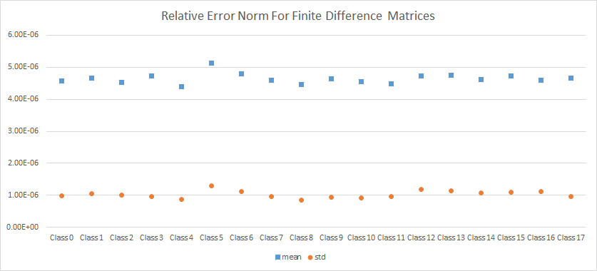
| SVD-generated Matrices | Laplacian Matrices | Finite Difference Matrices | ||||
| Class No. | Mean | Std | Mean | Std | Mean | Std |
| Class 0 | 3.54E-09 | 3.28E-09 | 4.10E-14 | 2.43E-13 | 1.61E-06 | 1.35E-06 |
| Class 0 | 1.07E-08 | 3.82E-09 | 2.05E-13 | 1.62E-13 | 4.58E-06 | 9.93E-07 |
| Class 1 | 1.16E-08 | 6.62E-09 | 6.07E-13 | 5.20E-13 | 4.67E-06 | 1.04E-06 |
| Class 2 | 1.23E-08 | 5.84E-09 | 1.69E-13 | 1.34E-13 | 4.52E-06 | 1.01E-06 |
| Class 3 | 1.25E-08 | 1.07E-08 | 2.46E-13 | 3.44E-13 | 4.72E-06 | 9.52E-07 |
| Class 4 | 1.13E-08 | 6.09E-09 | 1.93E-13 | 1.48E-13 | 4.38E-06 | 8.64E-07 |
| Class 5 | 1.12E-08 | 8.79E-09 | 9.25E-13 | 2.64E-12 | 5.12E-06 | 1.29E-06 |
| Class 6 | 1.16E-08 | 7.42E-09 | 5.51E-13 | 5.35E-13 | 4.79E-06 | 1.12E-06 |
| Class 7 | 1.33E-08 | 1.00E-08 | 1.98E-13 | 1.30E-13 | 4.60E-06 | 9.52E-07 |
| Class 8 | 1.08E-08 | 4.81E-09 | 2.09E-13 | 3.60E-13 | 4.47E-06 | 8.57E-07 |
| Class 9 | 1.18E-08 | 5.51E-09 | 1.87E-13 | 1.77E-13 | 4.63E-06 | 9.28E-07 |
| Class 10 | 1.18E-08 | 6.23E-09 | 1.78E-13 | 1.42E-13 | 4.55E-06 | 9.08E-07 |
| Class 11 | 1.28E-08 | 1.40E-08 | 2.33E-13 | 3.44E-13 | 4.49E-06 | 9.67E-07 |
| Class 12 | 1.43E-08 | 1.87E-08 | 1.78E-13 | 1.61E-13 | 4.74E-06 | 1.19E-06 |
| Class 13 | 1.22E-08 | 1.26E-08 | 2.21E-13 | 2.83E-13 | 4.75E-06 | 1.14E-06 |
| Class 14 | 1.51E-08 | 1.18E-08 | 3.57E-13 | 9.27E-13 | 4.61E-06 | 1.08E-06 |
| Class 15 | 1.19E-08 | 6.93E-09 | 2.24E-13 | 1.76E-13 | 4.74E-06 | 1.09E-06 |
| Class 16 | 1.26E-08 | 1.16E-08 | 2.15E-13 | 1.70E-13 | 4.59E-06 | 1.12E-06 |
| Class 17 | 1.31E-08 | 1.18E-08 | 1.25E-14 | 5.16E-14 | 1.83E-06 | 1.55E-06 |
The tests show quite accurate outputs even where we applied Algorithm 1.1 with very sparse multipliers of classes 13–17.
6 Conclusions: Sample Extension to the Computations for Least Squares Regression (LSR)
Our duality techniques for the average inputs can be extended to the acceleration of various matrix computations involving random multipliers. In this concluding section we describe such a sample extension to the following fundamental problem of matrix computations (cf. [GL13]).
Problem 6.1.
Least Squares Solution of an Overdetermined Linear System of Equations. Given two integers and such that , a matrix , and a vector , compute a vector that minimizes the norm .
If a matrix has full rank , then unique solution is given by the vector , satisfying the linear system of normal equations . Otherwise solution is not unique, and a solution having the minimum norm is given by the vector . In the important case where and an approximate solution is acceptable, Sarlós in [S06] proposed to simplify the computations as follows:
Algorithm 6.1.
Least Squares Regression (LSR).
- Initialization:
-
Fix an integer such that .
- Computations:
-
- 1.
Generate a scaled Gaussian matrix .
- 2.
Compute the matrix and the vector .
- 3.
Output a solution to the compressed Problem 6.1 where the matrix and the vector are replaced by the matrix and the vector , respectively.
- 1.
Now write and and compare the error norms (of the output of the latter algorithm) and (of the solution of the original Problem 6.1).
Theorem 6.1.
[W14, Theorem 2.3]. Suppose that we are given two tolerance values and , and , three integers , and such that and
for a certain constant , and a matrix . Then, with a probability at least , it holds that
for all matrices and all vectors normalized so that .
The theorem implies that with a probability at least , Algorithm 6.1 outputs an approximate solution to Problem 6.1 within the error norm bound provided that and .88 8 Such approximate solutions serve as preprocessors for practical implementation of numerical linear algebra algorithms for Problem 6.1 of least squares computation [M11, Section 4.5], [RT08], [AMT10].
For , the computational cost of performing the algorithm for approximate solution dramatically decreases versus the cost of computing exact solution, but can still be prohibitively high at the stage of computing the matrix product for . In a number of papers the former cost estimate has been dramatically decreased by means of replacing a multiplier with various random sparse and structured matrices (see [W14, Section 2.1]), for which the bound of Theorem 6.1 still holds for all matrices , although at the expense of increasing significantly the dimension .
Can we achieve similar progress without such an increase? [CW13] provides positive probabilistic answer based on the Johnson–Lindenstrauss Theorem, while the following theorem does this by using our duality approach in the case where is the average matrix in under the Gaussian probability distribution:
Theorem 6.2.
Dual LSR. The bound of Theorem 6.1 holds with a probability at least where and is an orthogonal matrix.
Proof.
Theorem 6.2 supports the computation of an approximate randomized solution of LSR Problem 6.1 for any orthogonal multiplier (e.g., an abridged scaled Hadamard’s multiplier or a count sketch multiplier) and for an input matrix average under the Gaussian probability distribution.
It follows that in this case Algorithm 6.1 can fail only for a narrow class of pairs and where denotes orthogonal matrices in and denotes matrices in , and even in the unlikely case of failure we can still have good chances for success if we apply heuristic recipes of our Section 2.
Appendix
Appendix A Randomized Matrix Computations
Theorem A.1.
Suppose that is an matrix of full rank , and are and matrices, respectively, for , and the entries of these two matrices are nonconstant linear combinations of finitely many i.i.d. random variables .
Then the matrices , , , and have full rank
(i) with probability 1 if are Gaussian variables and
(ii) with a probability at least if they are random variables sampled under the uniform probability distribution from a finite set having cardinality .
Proof.
The determinant, , of any block of a matrix , , , or is a polynomial of degree in the variables , and so the equation defines an algebraic variety of a lower dimension in the linear space of these variables (cf. [BV88, Proposition 1]). Clearly, such a variety has Lebesgue and Gaussian measures 0, both being absolutely continuous with respect to one another. This implies part (i) of the theorem. Derivation of part (ii) from a celebrated lemma of [DL78], also known from [Z79] and [S80], is a well-known pattern, specified in some detail in [PW08]. ∎
Lemma A.1.
(Rotational invariance of a Gaussian matrix.) Suppose that , , and are three positive integers, is an Gaussian matrix, and and are and orthogonal matrices, respectively.
Then and are Gaussian matrices.
We state the following estimates for real matrices, but similar estimates in the case of complex matrices can be found in [D88], [E88], [CD05], and [ES05]:
Definition A.1.
Norms of random matrices and expected value of a random variable. Write , , and , for a Gaussian matrix , and write for the expected value of a random variable . (, , and , for all pairs of and .)
Theorem A.2.
(Cf. [DS01, Theorem II.7].) Suppose that and are positive integers, , . Then
(i) Probability and
(ii) .
Theorem A.3.
Let denote the Gamma function and let . Then
(i) Probability for ,
(ii) Probability for ,
(iii) , provided that and .
Proof.
The probabilistic upper bounds of Theorem A.3 on are reasonable already in the case of square matrices, that is, where , but are strengthened very fast as the difference grows from 1.
Theorems A.2 and A.3 combined imply that an Gaussian matrix is well-conditioned unless the integer is large or the integer is close to 0. With some grain of salt we can still consider such a matrix well-conditioned even where the integer is small or vanishes provided that the integer is not large. Clearly, these properties can be extended immediately to all submatrices.
Acknowledgements: Our research has been supported by NSF Grant CCF 1116736 and PSC CUNY Award 68862–00 46. We are also grateful to Vsevolod Oparin for a pointer to relevant bibliography.
References
- [AMT10] H. Avron, P. Maymounkov, S. Toledo, Blendenpik: Supercharging LAPACK▓s Least-squares Solver, SIAM Journal on Scientific Computing, 32, 1217–1236, 2010.
- [AS00] N. Alon, J. Spencer, The Probabilistic Method, Wiley, 2000 (second edition).
- [B10] S. Börm, Efficient Numerical Methods for Non-local Operators: -Matrix Compression, Algorithms and Analysis, European Math. Society, 2010.
- [BBBDD14] M. Baboulin, D. Becker, G. Bosilca, A. Danalis, J. Dongarra, An Efficient Distributed Randomized Algorithm for Solving Large Dense Symmetric Indefinite Linear Systems, Parallel Computing (7th Workshop on Parallel Matrix Algorithms and Applications), 40, 7, 213–223, 2014.
- [BCDHKS14] G. Ballard, E. Carson, J. Demmel, M. Hoemmen, N. Knight, O. Schwartz, Communication Lower Bounds and Optimal Algorithms for Numerical Linear Algebra. Acta Numerica, 23, 1–155, 2014.
- [BGH03] S. Börm, L. Grasedyck, W. Hackbusch, Introduction to Hierarchical Matrices with Applications, Engineering Analysis with Boundary Elements, 27, 5, 405–422, 2003.
- [BGP05] A. Bini, L. Gemignani, V. Y. Pan, Fast and Stable QR Eigenvalue Algorithms for Generalized Semiseparable Matrices and Secular Equation, Numerische Mathematik, 100, 3, 373–408, 2005.
- [BV88] W. Bruns, U. Vetter, Determinantal Rings, Lecture Notes in Math., 1327, Springer, 1988.
- [C00] B. A. Cipra, The Best of the 20th Century: Editors Name Top 10 Algorithms, SIAM News (Society for Industrial and Applied Mathematics), 33, 4, 2, May 16, 2000.
- [CCF04] M. Charikar, K. Chen, M. Farach-Colton, Finding Frequent Items in Data Streams, Theoretical Computer Science, 312, 1, 3–15, 2004.
- [CD05] Z. Chen, J. J. Dongarra, Condition Numbers of Gaussian Random Matrices, SIAM. J. on Matrix Analysis and Applications, 27, 603–620, 2005.
- [CGR88] J. Carrier, L. Greengard, V. Rokhlin, A Fast Adaptive Algorithm for Particle Simulation, SIAM Journal on Scientific Computing, 9, 669–686, 1988.
- [CW13] K. L. Clarkson, D. P. Woodruff, Low Rank Approximation and Regression in Input Sparsity Time, Proceedings of the Forty-fifth Annual ACM Symposium on Theory of Computing (STOC ’13), 81–90, ACM New York, NY, USA, 2013. Full Version in arXiv:1207.6365.
- [D88] J. Demmel, The Probability That a Numerical Analysis Problem Is Difficult, Math. of Computation, 50, 449–480, 1988.
- [DE] Dillon Engineering, http://www.dilloneng.com/fft ip/parallel-fft.
- [DL78] R. A. Demillo, R. J. Lipton, A Probabilistic Remark on Algebraic Program Testing, Information Processing Letters, 7, 4, 193–195, 1978.
- [DS01] K. R. Davidson, S. J. Szarek, Local Operator Theory, Random Matrices, and Banach Spaces, in Handbook on the Geometry of Banach Spaces (W. B. Johnson and J. Lindenstrauss editors), pages 317–368, North Holland, Amsterdam, 2001.
- [E88] A. Edelman, Eigenvalues and Condition Numbers of Random Matrices, SIAM J. on Matrix Analysis and Applications, 9, 4, 543–560, 1988.
- [EGH13] Y. Eidelman, I. Gohberg, I. Haimovici, Separable Type Representations of Matrices and Fast Algorithms, volumes 1 and 2, Birkhäuser, 2013.
- [ES05] A. Edelman, B. D. Sutton, Tails of Condition Number Distributions, SIAM J. on Matrix Analysis and Applications, 27, 2, 547–560, 2005.
- [F77] R. Freivalds, Probabilistic Machines Can Use Less Running Time, IFIP Congress 1977, 839–842, 1977.
- [GH03] L. Grasedyck, W. Hackbusch, Construction and Arithmetics of H-Matrices, Computing, 70, 4, 295–334, 2003.
- [GL13] G. H. Golub, C. F. Van Loan, Matrix Computations, The Johns Hopkins University Press, Baltimore, Maryland, 2013 (fourth edition).
- [GR87] L. Greengard, V. Rokhlin, A Fast Algorithm for Particle Simulation, Journal of Computational Physics, 73, 325–348, 1987.
- [H02] N. J. Higham, Accuracy and Stability in Numerical Analysis, SIAM, Philadelphia, 2002.
- [HMST11] N. Halko, P. G. Martinsson, Y. Shkolnisky, M. Tygert, An Algorithm for the Principal Component Analysis of Large Data Sets, SIAM J. Scientific Computation, 33, 5, 2580–2594, 2011.
- [HMT11] N. Halko, P. G. Martinsson, J. A. Tropp, Finding Structure with Randomness: Probabilistic Algorithms for Approximate Matrix Decompositions, SIAM Review, 53, 2, 217–288, 2011.
- [M11] M. W. Mahoney, Randomized Algorithms for Matrices and Data, Foundations and Trends in Machine Learning, NOW Publishers, 3, 2, 2011. Preprint: arXiv:1104.5557 (2011) (Abridged version in: Advances in Machine Learning and Data Mining for Astronomy, edited by M. J. Way et al., pp. 647–672, 2012.)
- [MR95] R. Motwani, P. Raghavan, Randomized Algorithms, Cambridge UNiversity Press, 1995,
- [MRT05] P. G. Martinsson, V. Rokhlin, M. Tygert, A Fast Algorithm for the Inversion of General Toeplitz Matrices, Comput. Math. Appl., 50, 741–752, 2005.
- [P01]
V. Y. Pan,
Structured Matrices and Polynomials: Unified Superfast Algorithms,
Birkhäuser/Springer, Boston/New York, 2001. - [P15] V. Y. Pan, Transformations of Matrix Structures Work Again, Linear Algebra and Its Applications, 465, 1–32, 2015.
- [PQY15] V. Y. Pan, G. Qian, X. Yan, Random Multipliers Numerically Stabilize Gaussian and Block Gaussian Elimination: Proofs and an Extension to Low-rank Approximation, Linear Algebra and Its Applications, 481, 202–234, 2015.
- [PSZ15] V. Y. Pan, J. Svadlenka, L. Zhao, Estimating the Norms of Circulant and Toeplitz Random Matrices and Their Inverses, Linear Algebra and Its Applications, 468, 197–210, 2015.
- [PW08] V. Y. Pan, X. Wang, Degeneration of Integer Matrices Modulo an Integer, Linear Algebra and Its Applications, 429, 2113–2130, 2008.
- [PZ16] V. Y. Pan, L. Zhao, Low-rank Approximation of a Matrix: Novel Insights, New Progress, and Extensions, Proc. of the Eleventh International Computer Science Symposium in Russia (CSR’2016), (Alexander Kulikov and Gerhard Woeginger, editors), St. Petersburg, Russia, June 2016, Lecture Notes in Computer Science (LNCS), 9691, 352–366, Springer International Publishing, Switzerland (2016).
- [PZa] V. Y. Pan, L. Zhao, Numerically Safe Gaussian Elimination with No Pivoting, arxiv 1501.05385 CS, submitted on January 22, 2015, revised in June 2016.
- [RST09] V. Rokhlin, A. Szlam, M. Tygert, A Randomized Algorithm for Principal Component Analysis, SIAM Journal on Matrix Analysis and Applications, 31, 3, 1100–1124, 2009.
- [RT08] V. Rokhlin, M. Tygert, A Fast Randomized Algorithm for Overdetermined Linear Least-squares Regression, Proc. Natl. Acad. Sci. USA, 105, 36, 13212–13217, 2008.
- [S80] J. T. Schwartz, Fast Probabilistic Algorithms for Verification of Polynomial Identities, Journal of ACM, 27, 4, 701–717, 1980.
- [S98] G. W. Stewart, Matrix Algorithms, Vol I: Basic Decompositions, SIAM, Philadelphia, 1998.
- [S06] T. Sarlós, Improved Approximation Algorithms for Large Matrices via Random Projections, Proceedings of IEEE Symposium on Foundations of Computer Science (FOCS), 143–152, 2006.
- [SST06] A. Sankar, D. Spielman, S.-H. Teng, Smoothed Analysis of the Condition Numbers and Growth Factors of Matrices, SIAM J. on Matrix Analysis and Applics., 28, 2, 446–476, 2006.
- [T00] E.E. Tyrtyshnikov, Incomplete Cross-Approximation in the Mosaic-Skeleton Method, Computing, 64, 367–380, 2000.
- [T11] J. A. Tropp, Improved Analysis of the Subsampled Randomized Hadamard Transform, Adv. Adapt. Data Anal., 3, 1–2 (Special issue ”Sparse Representation of Data and Images”), 115–126, 2011. Also arXiv math.NA 1011.1595.
- [TZ12] M. Thorup, Y. Zhang, Tabulation-based 5-independent Hashing with Applications to Linear Probing and Second Moment Estimation, SIAM J. on Computing, 41, 2, 293–331, 2012.
- [VVGM05] R. Vandebril, M. Van Barel, G. Golub, N. Mastronardi, A Bibliography on Semiseparable Matrices, Calcolo, 42, 3–4, 249–270, 2005.
- [VVM07/08] R. Vandebril, M. Van Barel, N. Mastronardi, Matrix Computations and Semiseparable Matrices (Volumes 1 and 2), The Johns Hopkins University Press, Baltimore, Maryland, 2007.
- [VVVF10] M. Van Barel, R. Vandebril, P. Van Dooren, K. Frederix, Implicit Double Shift -algorithm for Companion Matrices, Numerische Mathematik, 116, 177–212, 2010.
- [W14] D.P. Woodruff, Sketching As a Tool for Numerical Linear Algebra, Foundations and Trends in Theoretical Computer Science, 10, 1–2, 1–157, 2014.
- [X12] J. Xia, On the Complexity of Some Hierarchical Structured Matrix Algorithms, SIAM J. Matrix Anal. Appl., 33, 388–410, 2012.
- [X13] J. Xia, Randomized Sparse Direct Solvers, SIAM J. Matrix Anal. Appl., 34, 197–227, 2013.
- [XXCB14] J. Xia, Y. Xi, S. Cauley, V. Balakrishnan, Superfast and Stable Structured Solvers for Toeplitz Least Squares via Randomized Sampling, SIAM J. Matrix Anal. Appl., 35, 44–72, 2014.
- [XXG12] J. Xia, Y. Xi, M. Gu, A Superfast Structured Solver for Toeplitz Linear Systems via Randomized Sampling, SIAM J. Matrix Anal. Appl., 33, 837–858, 2012.
- [Z79] R. E. Zippel, Probabilistic Algorithms for Sparse Polynomials, Proceedings of EUROSAM’79, Lecture Notes in Computer Science, 72, 216–226, Springer, Berlin, 1979.