Independent Resampling Sequential Monte Carlo Algorithms

Roland Lamberti Yohan Petetin François Desbouvries François Septier ^†^†thanks: R. Lamberti, Y. Petetin and F. Desbouvries are with Samovar, Telecom Sudparis, CNRS, Université Paris-Saclay, 9 rue Charles Fourier, 91011 Evry, France^†^†thanks: F. Septier is with Telecom Lille & UMR CNRS CRIStAL, Rue Guglielmo Marconi, 59653 Villeneuve d’Ascq, France

Abstract

Sequential Monte Carlo algorithms, or Particle Filters, are Bayesian filtering algorithms which propagate in time a discrete and random approximation of the a posteriori distribution of interest. Such algorithms are based on Importance Sampling with a bootstrap resampling step which aims at struggling against weights degeneracy. However, in some situations (informative measurements, high dimensional model), the resampling step can prove inefficient. In this paper, we revisit the fundamental resampling mechanism which leads us back to Rubin’s static resampling mechanism. We propose an alternative rejuvenation scheme in which the resampled particles share the same marginal distribution as in the classical setup, but are now independent. This set of independent particles provides a new alternative to compute a moment of the target distribution and the resulting estimate is analyzed through a CLT. We next adapt our results to the dynamic case and propose a particle filtering algorithm based on independent resampling. This algorithm can be seen as a particular auxiliary particle filter algorithm with a relevant choice of the first-stage weights and instrumental distributions. Finally we validate our results via simulations which carefully take into account the computational budget.

Index Terms:

Sequential Monte Carlo algorithms; Particle Filters; Importance Sampling; Auxiliary Particle Filter; Resampling.

I Introduction

Let $\{X_{k}\in\mathbb{R}^{m}\}_{k\geq 0}$ (resp. $\{Y_{k}\in\mathbb{R}^{n}\}_{k\geq 0}$ ) be a hidden (resp. observed) process. Let $X_{0:k}$ , say, denote $\{X_{i},0\leq i\leq k\}$ , $x_{0:k}=\{x_{i},0\leq i\leq k\}$ , and let $p(x)$ (resp. $p(x|y)$ ), say, denote the probability density function (pdf) of random variable (r.v.) $X$ (resp. of $X$ given $Y=y$ ); capital letters are used for r.v. and lower case ones for their realizations. We assume that $\{(X_{k},Y_{k})\}_{k\geq 0}$ is a Hidden Markov chain, i.e. that

\displaystyle p(x_{0:k},y_{0:k})=p(x_{0})\prod_{i=1}^{k}f_{i}(x_{i}|x_{i-1})\prod_{i=0}^{k}g_{i}(y_{i}|x_{i})\text{.}

(1)

Roughly speaking, pdf $f_{k}(x_{k}|x_{k-1})$ describes the dynamical evolution of the Markovian hidden process $\{X_{k}\}_{k\geq 0}$ between time $k-1$ and time $k$ while the likelihood $g_{k}(y_{k}|x_{k})$ describes the relation at time $k$ between an observation $y_{k}$ and the associated hidden state $x_{k}$ . We address the problem of computing a moment of some function $f({\bf.})$ w.r.t. the filtering pdf $p(x_{k}|y_{0:k})$ , i.e. the pdf of the hidden state given the past observations:

\Theta_{k}=\int f(x_{k})p(x_{k}|y_{0:k}){\rm d}x_{k}\text{.}

(2)

As is well known, $\Theta_{k}$ can be exactly computed only in very specific models, and one needs to resort to approximations in the general case. In this paper, we focus on a popular class of approximations called sequential Monte Carlo (SMC) algorithms or Particle Filters (PF), see e.g. [1, 2, 3] PF propagate over time a set of $N$ Monte Carlo (MC) weighted samples $\{w_{k}^{i},x_{k}^{i}\}_{i=1}^{N}$ which defines a discrete approximation $\sum_{i=1}^{N}w_{k}^{i}\delta_{x_{k}^{i}}$ of $p(x_{k}|y_{0:k})$ and enables to compute an estimate $\widehat{\Theta}_{k}$ of $\Theta_{k}$ :

\widehat{\Theta}_{k}=\sum_{i=1}^{N}w_{k}^{i}f(x_{k}^{i})\text{.}

(3)

More precisely, the computation of the set $\{w_{k}^{i},x_{k}^{i}\}_{i=1}^{N}$ is based on the sequential application of the Importance Sampling (IS) mechanism [4]. This mechanism consists in sampling particles according to an importance distribution and next weighting these samples in order to correct the discrepancy between the target and the importance distribution. However the direct sequential application of the IS mechanism in model (1) fails in practice since after a few time steps most weights get close to to zero, while only a few particles have non neglictible weights. Consequently IS alone becomes more and more inefficient since a lot of computational effort is devoted to sampling particles which will hardly contribute to the estimate $\widehat{\Theta}_{k}$ in (3).

As is well known, a traditional rescue against weights degeneracy consists in resampling the particles (- either at each time step or depending on some criterion such as the number of efficient particles [5] [6] [7] [8]), i.e. of re-drawing each particle with a probability equal to its weight. This yields the class of Sampling Importance Resampling (SIR) algorithms [9] [1] [10] [11]. This resampling (i.e., bootstrap) mechanism has proved to be beneficial in the long run, but its instantaneous effects are mitigated; though the resampling step indeed discards particles with low weights (such particles are likely never to be resampled), particles with significant weights are resampled several times, which results in dependency among the resampled points and support shrinkage. Consequently, particle filters based on the resampling mechanism can give poor results in some Markovian models (1), such as informative models where the likelihood $g_{k}(y_{k}|x_{k})$ is sharp. Our aim in this paper is thus to revisit this key rejuvenation scheme in order to design new PF algorithms which would keep the benefits of the resampling mechanism, while avoiding the local impoverishment of the resulting MC approximation of the filtering distribution.

To that end we begin with revisiting the SIR mechanism at one single time step $k\rightarrow k+1$ . This leads us back to an analysis of Rubin’s static SIR mechanism [12, §2] [13] [9] [14, §9.2], in which, roughly speaking, one obtains samples $x^{j}$ approximately drawn from a target distribution $p$ by drawing intermediate samples $\{\tilde{x}^{i}\}_{i=1}^{N}$ from an instrumental distribution $q$ , and next selecting $x^{j}$ among $\{\tilde{x}^{i}\}_{i=1}^{N}$ with a probability proportional to $\frac{p(\tilde{x}^{i})}{q(\tilde{x}^{i})}$ . We first observe that the samples $\{x^{j}\}$ produced by this SIR mechanism are dependent and marginally distributed from some compound pdf $\tilde{q}_{N}=\phi(p,q,N)$ which takes into account the effects of both pdfs $p$ and $q$ . Here the dependency is detrimental, because samples that would be i.i.d from $\tilde{q}_{N}$ would produce, whichever the number of sampled and resampled particles, a moment estimate with reduced variance; this result is further illustrated by a central limit theorem (CLT) which is compared to the existing CLTs for the static IS estimate (based on the pre-resampling samples $\{\tilde{x}^{i}\}_{i=1}^{N}$ ), on the one hand, and for the SIR estimate (based on the post-resampling ones $\{x^{j}\}_{j=1}^{M_{N}}$ ), on the other hand.

We next propose a procedure to obtain i.i.d. samples from $\tilde{q}_{N}$ , which leads to the computation of two point estimates of $\Theta=\int f(x)p(x){\rm d}x$ . The first one is based on unweighted i.i.d. samples and is an improved version of the classical (i.e., dependent) SIR estimate; the second one is based on post-resampling-weighted i.i.d. samples and can be seen as new IS estimate, based on the compound pdf $\tilde{q}_{N}$ . Finally we adapt these results to the sequential computation of $\Theta_{k}$ in model (1). We thus propose two new PF algorithms. One of them has an interesting interpretation in terms of Auxiliary Particle Filter (APF); more precisely, that algorithm naturally produces a relevant importance mixture distribution from which it is easy to sample. We finally illustrate our results via simulations, and carefully compare our algorithms with existing ones in terms of Root Mean Square Error (RMSE) and computational cost. The rest of this paper is organized as follows. Section II is devoted to the static case. In section III we address the sequential case, and derive new PF based on the results of section II. In section IV we perform simulations and discuss implementation issues, and we end the paper with a conclusion.

II IS with resampling viewed as a compound IS scheme

As recalled in the introduction, resampling from time to time is a standard rescue when applying IS in the sequential case. In this section we thus focus on one such time step $k\rightarrow k+1$ . This amounts to revisiting Rubin’s static SIR mechanism (see section (II-A)), which consists in resampling points $\{x_{i}\}_{i=1}^{M_{N}}$ from the weighted distribution $\sum_{i=1}^{N}w_{i}\delta_{\tilde{x}_{i}}$ where $\tilde{x}_{i}\stackrel{{\scriptstyle i.i.d.}}{{\sim}}q$ and the pre-resampling weights $w_{i}\propto\frac{p(\tilde{x}_{i})}{q(\tilde{x}_{i})}$ with $\sum_{i=1}^{N}w_{i}=1$ . As is well known, when $N\rightarrow\infty$ the resampled points $\{x_{i}\}_{i=1}^{M_{N}}$ become asymptotically i.i.d. from the target distribution $p$ . For finite $N$ however, these samples are dependent and drawn from some pdf $\tilde{q}_{N}$ which differs from $p$ and can indeed be seen as a compound IS density $\tilde{q}_{N}=\phi(p,q,N)$ produced by the succession of the sampling (S), weighting (W) and resampling (R) steps. We discuss on the benefits of drawing independent samples from $\tilde{q}_{N}$ (see section II-B), and next on reweighting these independent samples with post-resampling weights $w^{\prime}_{i}\propto\frac{p(x_{i})}{\tilde{q}_{N}(x_{i})}$ (see section II-C). In all this section we assume the scalar case for simplicity. We end the section with a summary (see section II-D).

II-A The dependent SIR mechanism

Let us begin with a brief review of Rubin’s classical SIR sampling mechanism and of the properties of the sampled and resampled particles.

II-A1 Properties of the sampled particles $\{\tilde{x}^{i}\}_{i=1}^{N}$

In the context of this paper we first recall the principle of IS. Let $p(x)$ be a probability density function and assume that we want to compute

\Theta=\int f(x)p(x){\rm d}x={\rm E}_{p}(f(X))\text{.}

(4)

In the Bayesian framework $p(x)$ is generally only known up to a constant, i.e. $p(x)\propto p_{u}(x)$ (subscript $u$ is for unnormalized) and it is not possible to obtain samples directly drawn from $p(x)$ . A solution is to introduce an importance distribution $q(x)$ which satisfies $q(x)>0$ when $p(x)>0$ and to rewrite $\Theta$ as the ratio of two expectations w.r.t. $q$ ,

\Theta=\frac{\int f(x)\frac{p_{u}(x)}{q(x)}q(x){\rm d}x}{\int\frac{p_{u}(x)}{q(x)}q(x){\rm d}x}=\frac{{\rm E}_{q}(f(X)\frac{p(X)}{q(X)})}{{\rm E}_{q}(\frac{p(X)}{q(X)})}\text{.}

(5)

Next, each expectation is approximated by a Monte Carlo method based on $N$ i.i.d. samples $(\tilde{x}^{1},\cdots,\tilde{x}^{N})$ drawn from $q(.)$ ; the IS estimate of $\Theta$ is given by

\widehat{\Theta}_{N}^{{\rm IS}}=\sum_{i=1}^{N}w^{i}f(\tilde{x}^{i})={\rm E}_{\hat{p}}(f(X))

(6)

where

\hat{p}(x)=\sum_{i=1}^{N}w^{i}\delta_{\tilde{x}^{i}}(x)

(7)

and where $w^{i}$ (the $i$ -th normalized importance weight) reads

w^{i}=\frac{\frac{p_{u}(\tilde{x}^{i})}{q(\tilde{x}^{i})}}{\sum_{j=1}^{N}\frac{p_{u}(\tilde{x}^{j})}{q(\tilde{x}^{j})}}=\frac{\frac{p(\tilde{x}^{i})}{q(\tilde{x}^{i})}}{\sum_{j=1}^{N}\frac{p(\tilde{x}^{j})}{q(\tilde{x}^{j})}}\text{.}

(8)

As is well known [4], under mild assumptions

\widehat{\Theta}_{N}^{{\rm IS}}\stackrel{{\scriptstyle\rm a.s.}}{{\rightarrow}}\Theta,

(9)

and a CLT is available too ( ${\mathcal{D}}{\rightarrow}$ denotes the convergence in distribution):

\sqrt{N}(\widehat{\Theta}^{\rm IS}_{N}-\Theta)\overset{\mathcal{D}}{\rightarrow}\mathcal{N}\left(0,{\rm E}_{q}\left(\frac{p^{2}(X)}{q^{2}(X)}(f(X)-\Theta)^{2}\right)\right).

(10)

II-A2 Properties of the resampled particles $\{x^{i}\}_{i=1}^{M_{N}}$

From (9) and (10), $\hat{p}$ can be seen as a discrete approximation of the target density $p$ , and one expects that for large $N$ , (re)sampling from $\hat{p}$ would produce samples approximately drawn from $p$ . This is the rationale of Rubin’s SIR mechanism [12, §2], [13], [9], [14, §9.2]. More precisely, let us as above draw $N$ i.i.d. samples $\tilde{x}^{i}$ from $q$ , and next $M_{N}$ i.i.d samples $x^{i}$ from $\hat{p}$ in (7). It is indeed well-known (see [9] [12]) that when $N\rightarrow\infty$ , each r.v. $x^{i}$ produced by this mechanism converges in distribution to $p(.)$ , so Rubin’s technique can be seen as a two-step sampling mechanism which transforms samples drawn from $q$ into samples (approximately) drawn from $p$ .

This convergence result can be completed by a CLT which involves the estimate of $\Theta$ based on the unweighted set $\{(\frac{1}{M_{N}},x^{i})\}_{i=1}^{M_{N}}$ :

\widehat{\Theta}^{\rm SIR}_{M_{N}}=\frac{1}{M_{N}}\sum_{i=1}^{M_{N}}f(x^{i})\text{.}

(11)

Let $N\rightarrow\infty$ , let $M_{N}$ be a non decreasing sequence with $M_{N}\rightarrow\infty$ , and let ${\rm lim}\frac{N}{M_{N}}=\alpha>0$ (possibly $\infty$ ); then under mild conditions (see e.g. [14, §9])

\displaystyle\sqrt{M_{N}}(\widehat{\Theta}^{\rm SIR}_{M_{N}}-\Theta)

\displaystyle\overset{\mathcal{D}}{\rightarrow}\mathcal{N}(0,{\rm var}_{p}(f(X))+\alpha^{-1}{\rm E}_{q}\left((\frac{p^{2}(X)}{q^{2}(X)}(f(X)-\Theta)^{2})\right))\text{.}

(12)

If $\alpha\rightarrow\infty$ then the asymptotic variance tends to ${\rm var}_{p}(f(X))$ , which shows that the SIR estimate asymptotically has the same behavior as a crude Monte Carlo estimate directly deduced from $M_{N}$ samples according to the target distribution $p(.)$ , provided the number $N$ of intermediate samples is large compared to $M_{N}$ .

However, for computational reasons, the number of samples $N$ and $M_{N}$ should not be too large in practice. Consequently we now focus on the samples produced by the SIR procedure from a non asymptotical point of view and we have the following result (the proof is given in the Appendix).

Proposition 1

Let us consider the samples $\{x^{i}\}_{i=1}^{M_{N}}$ produced by the SIR mechanism described above. Then these samples are identically distributed according to a pdf $\tilde{q}_{N}$ , with

	$\displaystyle\tilde{q}_{N}(x)$	$\displaystyle=$	$\displaystyle Nh_{N}(x)q(x)\text{,}$		(13)
	$\displaystyle h_{N}(x)$	$\displaystyle=$	$\displaystyle\int\int\frac{\frac{p(x)}{q(x)}}{\frac{p(x)}{q(x)}+\sum_{l=1}^{N-1}\frac{p(x^{l})}{q(x^{l})}}\prod_{l=1}^{N-1}q(x^{l}){\rm d}x^{l}\text{.}$		(14)

So for fixed sample size $N$ , the SIR mechanism produces dependent samples $\{x^{i}\}_{i=1}^{M_{N}}$ distributed from $\tilde{q}_{N}$ (these samples are independent given the intermediate set $\{\tilde{x}^{i}\}_{i=1}^{N}$ , but become dependent when this conditioning is removed). In practice, this dependency results in support shrinkage since, by construction, an intermediate sample $\tilde{x}^{i}$ can be resampled several times, and $\{x^{i}\}_{i=1}^{M_{N}}$ is a subset of $\{\tilde{x}^{i}\}_{i=1}^{N}$ . For instance let $M_{N}=N$ . If we assume that $w^{j}=1$ for some $j$ and $w^{i}=0$ for $i\neq j$ , then $x^{i}=\tilde{x}^{j}$ for all $i$ . By contrast, if $w^{i}=1/N$ for all $i$ , then the average number of different samples $\{x^{i}\}_{i=1}^{N}$ is approximately $N/3$ [15]. Nevertheless the resampling step remains useful in a dynamic setup (see section III): even though locally it leads to an impoverishment of the diversity, this step is critical for recreating diversity at the next time step.

II-B The independent SIR mechanism

Observe that the two factors in (13) reflect the effects of the sampling and resampling step: pdf $q$ is used in the S step, while $h_{N}(x)$ , which can be interpreted as the conditional expectation of a normalized importance weight when its associated particle is $x$ , results from the (W,R) steps. So particles drawn from $\tilde{q}_{N}$ are likely to be in regions where 1) $q$ is large (since these particles have first been sampled); and 2) which have also been resampled because their associated weight was large enough. Now our objective is to propose an alternative mechanism which, in the sequential case, will produce the same positive effect as the classical SIR mechanism (i.e. fighting against weight degeneracy by eliminating the samples with weak importance weights), while ensuring the diversity of the final support. Such a support diversity is ensured if we draw samples independently from the continuous pdf $\tilde{q}_{N}(.)$ . We first study the potential benefits of this sampling mechanism (see section II-B1) and next discuss its implementation (see section II-B2).

II-B1 Statistical properties

Let us now assume that we have at our disposal a set of $M_{N}$ i.i.d. samples $\{\overline{x}^{i}\}_{i=1}^{M_{N}}$ drawn from $\tilde{q}_{N}(.)$ defined in (13) (14). Before addressing the practical computation of such a set (see section II-B2), let us study its properties by considering the crude estimate of $\Theta$ based on these $M_{N}$ i.i.d samples:

\widehat{\Theta}^{\rm I-SIR}_{M_{N}}=\frac{1}{M_{N}}\sum_{i=1}^{M_{N}}f(\overline{X}^{i})\text{.}

(15)

(I in notation I-SIR stands for independent). Our aim is to compare $\widehat{\Theta}^{\rm I-SIR}_{M_{N}}$ to $\widehat{\Theta}^{\rm SIR}_{M_{N}}$ , and more generally $\widehat{\Theta}^{\rm IS}_{N}$ , $\widehat{\Theta}^{\rm SIR}_{M_{N}}$ and $\widehat{\Theta}^{\rm I-SIR}_{M_{N}}$ . We first have the following result (the proof is given in the Appendix).

Proposition 2

Let us consider the three estimates $\widehat{\Theta}^{\rm IS}_{N}$ , $\widehat{\Theta}^{\rm SIR}_{M_{N}}$ and $\widehat{\Theta}^{\rm I-SIR}_{M_{N}}$ defined in (6), (11) and (15) respectively. Then

	$\displaystyle{\rm E}(\widehat{\Theta}^{\rm IS}_{N})$	$\displaystyle=$	$\displaystyle{\rm E}(\widehat{\Theta}^{\rm SIR}_{M_{N}})={\rm E}(\widehat{\Theta}^{\rm I-SIR}_{M_{N}})\text{,}$		(16)
	$\displaystyle{\rm var}(\widehat{\Theta}^{\rm SIR}_{M_{N}})$	$\displaystyle=$	$\displaystyle{\rm var}(\widehat{\Theta}^{\rm I-SIR}_{M_{N}})+\frac{M_{N}-1}{M_{N}}{\rm var}(\widehat{\Theta}^{\rm IS}_{N})\text{.}$		(17)

Equation (17) ensures that an estimate based on independent samples obtained from $\tilde{q}_{N}$ outperforms the classical SIR estimate; the gain of $\widehat{\Theta}^{\rm I-SIR}_{M_{N}}$ w.r.t. $\widehat{\Theta}^{\rm SIR}_{M_{N}}$ depends on the variance of ${\rm var}(\widehat{\Theta}^{\rm IS}_{N})$ . On the other hand it is well known (see e.g. [14, p. 213]) that ${\rm var}(\widehat{\Theta}^{\rm SIR}_{M_{N}})=$ ${\rm var}(\widehat{\Theta}^{\rm IS}_{N})+{\rm E}({\rm var}(\widehat{\Theta}^{\rm SIR}_{M_{N}}|\{\tilde{x}^{i}\}_{i=1}^{N}))$ ; so both $\widehat{\Theta}^{\rm I-SIR}_{M_{N}}$ and $\widehat{\Theta}^{\rm IS}_{N}$ are preferable to $\widehat{\Theta}^{\rm SIR}_{M_{N}}$ .

On the other hand, comparing the variance of $\widehat{\Theta}^{\rm IS}_{N}$ to that of $\widehat{\Theta}^{\rm I-SIR}_{M_{N}}$ is more difficult, because we have to compare $\frac{1}{M_{N}}{\rm var}_{\tilde{q}_{N}}(f(\overline{X}))$ to ${\rm var}(\sum_{i=1}^{N}w^{i}(\tilde{X}^{1},\cdots,\tilde{X}^{N})f(\tilde{X}_{i}))$ where $\tilde{X}^{i}\overset{\rm i.i.d}{\sim}q(.)$ . However, we have the following CLT (the proof is given in the Appendix).

Theorem 1

Let us consider the independent SIR estimate defined in (15). Let assume that $N\rightarrow\infty$ , $M_{N}$ is a non decreasing sequence with $M_{N}\rightarrow\infty$ and $\displaystyle{\lim_{N\rightarrow\infty}}\frac{N}{M_{N}}=\alpha>0$ . Then $\widehat{\Theta}^{\rm I-SIR}_{M_{N}}$ satisfies

\sqrt{M_{N}}(\widehat{\Theta}^{\rm I-SIR}_{M_{N}}-\Theta)\overset{\mathcal{D}}{\rightarrow}\mathcal{N}\left(0,{\rm var}_{p}(f(X))\right)\text{.}

(18)

Let us comment this result. First Theorem 1 enables again to compare $\widehat{\Theta}^{\rm I-SIR}_{M_{N}}$ to $\widehat{\Theta}^{\rm SIR}_{M_{N}}$ . Comparing (12) and (18) confirms (17), since the asymptotic variance of $\widehat{\Theta}^{\rm I-SIR}_{M_{N}}$ is always lower than that of $\widehat{\Theta}^{\rm SIR}_{M_{N}}$ . Also note that in the independent case the asymptotic variance of $\widehat{\Theta}^{\rm I-SIR}_{M_{N}}$ no longer depends on $\alpha>0$ .

Next Theorem 1 also gives some elements for comparing $\widehat{\Theta}^{\rm I-SIR}_{M_{N}}$ to $\widehat{\Theta}^{\rm IS}_{N}$ . Let for simplicity $M_{N}=N$ . Then the comparison of both estimates relies on that of the asymptotic variances in (10) and (18):

	$\displaystyle\sigma^{2,\rm IS}_{\infty}(q)$	$\displaystyle=$	$\displaystyle{\rm E}_{q}\left(\frac{p^{2}(X)}{q^{2}(X)}(f(X)-\Theta)^{2}\right),$		(19)
	$\displaystyle\sigma^{2,\rm I-SIR}_{\infty}$	$\displaystyle=$	$\displaystyle{\rm var}_{p}(f(X)).$		(20)

For a given target pdf $p({\bf.})$ and function $f({\bf.})$ , $\sigma^{2,\rm IS}_{\infty}(q)$ depends on the importance pdf $q({\bf.})$ and is well known [16, §2.9] [4, Theorem 3] to be minimum for $q^{\star}(x)\propto p(x)|f(x)-\Theta|$ ; for that $q^{\star}$ , $\sigma^{2,{\rm IS}}_{\infty}(q^{\star})=(\int|f(x)-\Theta|p(x){\rm d}x)^{2}\leq{\rm var}_{p}(f(X))$ , so $\widehat{\Theta}^{\rm IS}_{N}(q^{\star})$ outperforms $\widehat{\Theta}^{\rm I-SIR}_{N}$ for large values of $N$ . On the other hand for other importance distributions $\sigma^{2,\rm IS}_{\infty}(q)$ may become larger than $\sigma^{2,\rm I-SIR}_{\infty}$ . Also note that the variances in (19) and (20) depend on function $f({\bf.})$ ; on the other hand, for large $N$ , $\widehat{\Theta}^{\rm I-SIR}_{N}$ has the same behavior as a crude estimate built from samples drawn from $p(.)$ and so is adapted for a large class of functions $f({\bf.})$ .

II-B2 Sampling procedure

It remains to describe a procedure to obtain i.i.d. samples from $\tilde{q}_{N}$ . Algorithm 1 ensures that the final samples $\{x^{i},\cdots,x^{M_{N}}\}$ are drawn independently from $\tilde{q}_{N}$ .

Input : an importance distribution

q

N

and

M_{N}

Result:

\{x^{i}\}_{i=1}^{M_{N}}

\overset{\rm i.i.d.}{\sim}\tilde{q}_{N}

for $1\leq i\leq M_{N}$ do

for $1\leq j\leq N$ do

\tilde{x}^{i,j}\sim q(.)

;

w^{i,j}\propto p_{u}(\tilde{x}^{i,j})/q(\tilde{x}^{i,j})

\sum_{j=1}^{N}w^{i,j}=1

;

end for

x^{i}\sim\sum_{j=1}^{N}w^{i,j}\delta_{\tilde{x}^{i,j}}

end for

Algorithm 1 The independent SIR algorithm

Compared to the classical SIR procedure, the independent SIR algorithm described in Algorithm 1 relies on a sampling step of $N\times M_{N}$ intermediate samples $\tilde{x}$ and $M_{N}$ independent resampling steps. Consequently, for a given budget of sampling and resampling steps, the independent procedure should be compared with a classical SIR one in which we sample $N\times M_{N}$ points and resample $M_{N}$ of them. In this last case, we obtain $M_{N}$ dependent samples drawn from $\tilde{q}_{N\times M_{N}}$ . First, using (12) with $\alpha=\lim_{N\rightarrow\infty}\frac{N\times M_{N}}{M_{N}}=\infty$ , we see that both estimates $\widehat{\Theta}^{\rm I-SIR}_{M_{N}}$ and $\widehat{\Theta}^{\rm SIR}_{M_{N}}$ with $N\times M_{N}$ intermediate samples have the same asymptotic behavior. However the independent procedure can be easily parallelized because the resampling steps are by nature independent contrary to the SIR procedure where the $N\times M_{N}$ intermediate samples are directly resampled.

II-C Reweighting the independent samples?

We finally discuss the final weights which are attributed to the resampled particles. In the SIR procedure, each final sample is weighted by $1/M_{N}$ . From an IS point of view, this weighting traduces the fact that the final samples become drawn from the target distribution $p(.)$ and independent when $N\rightarrow\infty$ [12]. Moreover the convergence results of $\widehat{\Theta}^{\rm I-SIR}_{M_{N}}$ to $\Theta$ (see e.g. [17] [14]) confirm that these weights are valid from an asymptotical point of view. In the independent SIR procedure, the only difference is that the final samples are independent, even from a non-asymptotical point of view.

Now, if $N$ is finite, one can wonder if weights $1/M_{N}$ are optimal. In Algorithm 1, samples $\{X^{i}\}_{i=1}^{M_{N}}$ are independent and sampled from $\tilde{q}_{N}$ . Consequently, for a given $N$ , $\tilde{q}_{N}$ can be seen as a post-resampling compound importance distribution $\tilde{q}_{N}=\phi(p,q,N)$ , and a final sample $x^{i}$ should be weighted by a post-resampling weight proportional to $p_{u}(x^{i})/\tilde{q}_{N}(x^{i})$ . This yields a new estimate $\widehat{\Theta}^{\rm I-SIR-w}$ of (4) (superscript $w$ stands for weighted)

\widehat{\Theta}^{\rm I-SIR-w}_{M_{N}}=\sum_{i=1}^{M_{N}}\frac{\frac{p_{u}(x^{i})}{\tilde{q}_{N}(x^{i})}}{\sum_{j=1}^{M_{N}}\frac{p_{u}(x^{j})}{\tilde{q}_{N}(x^{j})}}f(x^{i})\text{,}

(21)

which coincides with the IS estimate (6) with importance distribution $\tilde{q}_{N}(.)$ . It is difficult to compare $\widehat{\Theta}^{\rm I-SIR}_{M_{N}}$ and $\widehat{\Theta}^{\rm I-SIR-w}_{M_{N}}$ because the expression of the weights in this last case depends on $N$ . However, it is interesting to note that contrary to $\widehat{\Theta}^{\rm I-SIR}_{M_{N}}$ , $M_{N}$ impacts the bias of the estimate $\widehat{\Theta}^{\rm I-SIR-w}_{M_{N}}$ . For example, if we set $N=1$ (so $q_{N}=q$ ) and $M_{1}$ is arbitrary then $\widehat{\Theta}^{\rm I-SIR-w}_{M_{1}}$ coincides with the IS estimate with $M_{1}$ i.i.d. samples drawn from $q$ while the unweighted estimate $\widehat{\Theta}^{\rm I-SIR}_{M_{1}}$ is a crude estimate of $\int f(x)q(x){\rm d}x$ and is not adapted for the estimation of $\Theta$ . More generally, using the delta method to approximate ${\rm E}(\widehat{\Theta}^{\rm I-SIR}_{M_{N}})$ and ${\rm E}(\widehat{\Theta}^{\rm I-SIR-w}_{M_{N}})$ [18] we observe that

		$\displaystyle{\rm E}(\widehat{\Theta}^{\rm I-SIR}_{M_{N}})\!=\!{\rm E}(\widehat{\Theta}^{\rm IS}_{N})\!\approx\!\Theta\!-\!\frac{1}{N}{\rm E}_{q}\left(\frac{p^{2}(X)}{q^{2}(X)}(f(x)\!-\!\Theta)\right)\!\!\text{,}$		(22)
		$\displaystyle{\rm E}(\widehat{\Theta}^{\rm I-SIR-w}_{M_{N}})\!\approx\!\Theta\!-\!\frac{1}{M_{N}}{\rm E}_{\tilde{q}_{N}}\left(\frac{p^{2}(X)}{\tilde{q}_{N}^{2}(X)}(f(x)-\Theta)\right)\text{.}$		(23)

So for a fixed number of sampled points $N$ , we see that in the unweighted case the bias of $\widehat{\Theta}^{\rm I-SIR}_{M_{N}}$ is independent of $M_{N}$ . By contrast, whichever $N$ the bias of ${\rm E}(\widehat{\Theta}^{\rm I-SIR-w}_{M_{N}})$ tends to $0$ as $M_{N}\rightarrow\infty$ .

Finally, it remains to compute $p_{u}(x^{i})/\tilde{q}_{N}(x^{i})$ in practice. In general, $\tilde{q}_{N}$ in (13) is not available in close form because it relies on the integral $h_{N}(x)$ in (14). However, the $N\times M_{N}$ intermediate samples which have been used in Algorithm 1 can be recycled to approximate the conditional expectation $h_{N}(x)$ . For a given $x$ and using the intermediate samples $\tilde{x}^{i,j}$ of Algorithm 1, a crude Monte Carlo estimate of $h_{N}(x)$ reads

\hat{h}_{N}(x)=\sum_{i=1}^{M_{N}}\frac{\frac{p_{u}(x)}{q(x)}}{\frac{p_{u}(x)}{q(x)}+\sum_{j=1}^{N-1}\frac{p_{u}(\tilde{x}^{i,j})}{q(\tilde{x}^{i,j})}}\text{.}

(24)

Importance weights $\frac{p_{u}(x)}{\tilde{q}_{N}(x)}$ in (21) can be approximated by $\frac{p_{u}(x)}{N\hat{h}_{N}(x)q(x)}$ . Note that the computation of these approximated weights do not require extra computational cost since $p_{u}(\tilde{x}^{i,j})/q(\tilde{x}^{i,j})$ has already been computed in Algorithm 1 to obtain i.i.d. samples.

II-D Summary

In summary, we now have at our disposal four estimates to compute $\Theta$ in (4) from an importance distribution $q(.)$ . $\widehat{\Theta}^{\rm IS}_{N}$ and $\widehat{\Theta}^{\rm SIR}_{M_{N}}$ are deduced from the IS and Rubin’s SIR mechanisms, respectively. $\widehat{\Theta}^{\rm SIR}_{M_{N}}$ relies on unweighted dependent samples from $\tilde{q}_{N}$ . Using unweighted independent samples from $\tilde{q}_{N}$ produces the estimate $\widehat{\Theta}^{\rm I-SIR}_{M_{N}}$ which outperforms $\widehat{\Theta}^{\rm SIR}_{M_{N}}$ and possibly $\widehat{\Theta}^{\rm IS}_{N}$ ; it also becomes asymptotically independent of the choice of the initial importance distribution $q(.)$ according to theorem 1. This estimate does not suffer from the support impoverishment caused by the resampling step. On the other hand it requires a larger computational cost which, however, can be exploited in order to associate to the i.i.d. samples post-resampling importance weights based on the $\tilde{q}_{N}(x)$ . We thus obtain a weighted estimate $\widehat{\Theta}^{\rm I-SIR-w}_{M_{N}}$ which can be seen as the estimate deduced from the IS mechanism based on the compound IS distribution $\tilde{q}_{N}(x)$ . We will compare these estimates via simulations and will take into account their computational cost in Section IV-A.

III Independent resampling based PF

We now adapt the results of Section II to the Bayesian filtering problem. In section III-A we briefly recall the principle of classical SIR algorithms which are based on dependent resampling. Our SIR algorithm with independent resampling and unweighted samples is proposed in section III-B. However, computing the post-resampling weights is more challenging here than in the static case because the pdf $\tilde{q}_{N}$ of the static case becomes a sum of $N$ terms which should be computed for each final sample. So in section III-C we revisit the algorithm of section III-B in terms of APF. We first observe that the independent SIR algorithm can be seen as the first step of an APF algorithm since it implicitly draws samples from a mixture pdf. Making full use of the APF methodology enables us to weight our final samples.

III-A Classical SIR algorithms (based on dependent resampling)

We now assume that we are given some hidden Markov model (1) and we briefly recall how $\Theta_{k}$ in (2) can be computed recursively via PF. PF relies on the sequential application of the normalized IS mechanism described in Section II-A for the target distribution $p(x_{0:k}|y_{0:k})$ which is known up to a constant according to (1). Let $q(x_{0:k})$ be an importance distribution ( $q(x_{0:k})$ can depend on $y_{0:k}$ but this dependency is not written here to avoid notational burden). Starting from $N$ weighted trajectories $x_{0:k-1}^{i}$ sampled from $q(x_{0:k-1})$ , we first extend each trajectory $x_{0:k-1}^{i}$ by a particle $\tilde{x}_{k}^{i}$ sampled from $q(x_{k}|x_{0:k-1}^{i})$ and next update the old weights $w_{k-1}^{i}$ via

w_{k}^{i}\propto w_{k-1}^{i}\frac{f_{k}(\tilde{x}_{k}^{i}|x_{k-1}^{i})g_{k}(y_{k}|\tilde{x}_{k}^{i})}{q(\tilde{x}_{k}^{i}|x_{0:k-1}^{i})},\sum_{i=1}^{N}w_{k}^{i}=1\text{.}

(25)

Unfortunately, it is well-known that this direct sequential application of IS leads to weight degeneracy: after a few iterations only few weights $w_{k}^{i}$ have a non null value [19]. A traditional rescue consists in resampling, either systematically or according to some criterion such as the Effective Sample Size [5] [6] which is approximated by $1/\sum_{i=1}^{N}(w_{k}^{i})^{2}$ . The corresponding algorithm is given in Algorithm 2 and we shall assume that the size $N$ of the MC approximation remains constant thoughout the iterations. Finally Algorithm 2 enables to compute two estimates of $\Theta_{k}$ :

	$\displaystyle\widehat{\Theta}_{N,k}^{\rm SIS}$	$\displaystyle=$	$\displaystyle\sum_{i=1}^{N}w_{k}^{i}f(\tilde{X}_{k}^{i})\text{,}$		(26)
	$\displaystyle\widehat{\Theta}_{N,k}^{\rm SIR}$	$\displaystyle=$	$\displaystyle\frac{1}{N}\sum_{i=1}^{N}f(X_{k}^{i})\text{.}$		(27)

As is well known, the pre-resampling estimator $\widehat{\Theta}_{N,k}^{\rm SIS}$ is preferable to the post-resampling one $\widehat{\Theta}_{N,k}^{\rm SIR}$ and should be used in practice; but $\widehat{\Theta}_{N,k}^{\rm SIR}$ is recalled here because it will be compared below to the independent resampling estimator (32).

Input :

q(x_{k}|x_{0:k-1})

y_{k}

\{w_{k-1}^{i},x_{0:k-1}^{i}\}_{i=1}^{N}

Result:

\{w_{k}^{i},x_{0:k}^{i}\}_{i=1}^{N}

for $1\leq i\leq N$ do

\tilde{x_{k}}^{i}\sim q(x_{k}|x_{0:k-1}^{i})

;

w_{k}^{i}\propto w_{k-1}^{i}\frac{f_{k}(\tilde{x}_{k}^{i}|x_{k-1}^{i})g_{k}(y_{k}|\tilde{x}_{k}^{i})}{q(\tilde{x}_{k}^{i}|x_{0:k-1}^{i})}

\sum_{i=1}^{N}w_{k}^{i}=1

;

end for

if Resampling then

for $1\leq i\leq N$ do

l^{i}\sim{\rm Pr}(L=l|\{x_{0:k-1}^{j},\tilde{x}_{k}^{j}\}_{j=1}^{N})=w_{k}^{l}

Set

x_{0:k}^{i}=(x_{0:k-1}^{l^{i}},\tilde{x}_{k}^{l^{i}})

w_{k}^{i}=\frac{1}{N}

end for

else

Set

\{x_{k}^{i}\}_{i=1}^{N}=\{\tilde{x}_{k}^{i}\}_{i=1}^{N}

end if

Algorithm 2 The classical SIR algorithm (based on dependent resampling)

In practice, it remains to choose the conditional importance distribution $q(x_{k}|x_{0:k-1})$ . A popular solution consists in choosing $q(x_{k}|x_{0:k-1})=f_{k}(x_{k}|x_{k-1})$ , since this pdf is part of model (1) and is generally easy to sample from; another one is the so-called optimal conditional importance distribution $q(x_{k}|x_{0:k-1})=p(x_{k}|x_{k-1},y_{k})$ which takes into account the new observation $y_{k}$ and for which weights $w_{k}^{i}$ no longer depend on the sampled particles $\{\tilde{x}_{k}^{i}\}_{i=1}^{N}$ . The optimal conditional importance distribution is generally not available in closed form but some approximation techniques have been proposed, see e.g. [19] [20] [21]. The choice of the importance distribution will be not discussed in this paper and does not impact the proposed methodology. Finally, let us mention that convergence results are also available for the PF presented in Algorithm 2, see e.g. [22] [23] [17] [14]. Some of them are based on the recursive application of the CLTs recalled in Section II.

III-B An alternative SIR algorithm (based on independent resampling)

Let us first adapt Proposition 1 to the sequential context. So we address the conditional distribution given $\{x_{0:k-1}^{i}\}_{i=1}^{N}$ of the resampled particles $X_{k}^{i}$ and we have the following result (the proof is omitted).

Proposition 3

Let us consider the samples $\{X_{k}^{i}\}_{i=1}^{N}$ produced by the SIR mechanism of Algorithm 2. Let

	$\displaystyle p_{i,k}(x)$	$\displaystyle=$	$\displaystyle w_{k-1}^{i}f_{k}(x\|x_{k-1}^{i})g_{k}(y_{k}\|x)\text{,}$		(28)
	$\displaystyle q_{i,k}(x)$	$\displaystyle=$	$\displaystyle q(x\|x_{0:k-1}^{i})\text{.}$		(29)

Then given the initial trajectories $\{x_{0:k-1}^{i}\}_{i=1}^{N}$ , the new samples $\{X_{k}^{i}\}_{i=1}^{N}$ are identically distributed according to a pdf $\tilde{q}_{N,k}$ which reads

\displaystyle\tilde{q}_{N,k}(x)=\sum_{i=1}^{N}h_{i,k}(x)q_{i,k}(x)\text{,}

(30)

where $h_{i,k}(x)$ coincides with the conditional expectation (given $(X_{k}^{i}=x)$ ) of the $i$ -th importance weight at time $k$ ,

h_{i,k}(x)=\int\int\frac{\frac{p{i,k}(x)}{q_{i,k}(x)}}{\frac{p_{i,k}(x)}{q_{i,k}(x)}+\sum_{l\neq i}\frac{p_{l,k}(x^{l})}{q_{l,k}(x^{l})}}\prod_{l\neq i}q_{l,k}(x^{l}){\rm d}x^{l}\text{.}

(31)

Note that in this proposition we focus on the distribution of $X_{k}^{i}$ given $\{x_{0:k-1}^{i}\}_{i=1}^{N}$ . Given $\{x_{0:k-1}^{i},\tilde{x}_{k}^{i}\}_{i=1}^{N}$ , the new samples $\{X_{k}^{i}\}_{i=1}^{N}$ are independent; when we remove the dependency in $\{\tilde{x}_{k}^{i}\}_{i=1}^{N}$ , $\{X_{k}^{i}\}_{i=1}^{N}$ become identically distributed according to $\tilde{q}_{N,k}$ but are dependent (a same particle can be resampled several times).

Since $\tilde{q}_{N,k}$ is a pdf, a procedure which would produce samples conditionally i.i.d. from $\tilde{q}_{N,k}$ would enable us to keep the advantage of the resampling step, i.e. to recreate diversity for the next time iteration while avoiding local impoverishment of the support. Except in a particular case which will be described later, sampling directly from $\tilde{q}_{N,k}(x)$ is difficult for an arbitrary conditional importance distribution $q(x_{k}|x_{0:k-1})$ . We thus propose a procedure similar to Algorithm 1 but adapted to the dynamical context. The SIR algorithm with independent resampling is given by Algorithm 3. Note that a difference with Algorithm 2 is that the distribution of the discrete index $L^{i}$ now depends on $i$ .

Input :

q(x_{k}|x_{0:k-1})

y_{k}

\{w_{k-1}^{i},x_{0:k-1}^{i}\}_{i=1}^{N}

Result:

\{w_{k}^{i},x_{0:k}^{i}\}_{i=1}^{N}

for $1\leq i\leq N$ do

for $1\leq j\leq N$ do

\tilde{x_{k}}^{i,j}\sim q(x_{k}|x_{0:k-1}^{i})

;

w_{k}^{i,j}\propto\frac{f_{k}(\tilde{x}_{k}^{i,j}|x_{k-1}^{i})g_{k}(y_{k}|\tilde{x}_{k}^{i,j})}{q(\tilde{x}_{k}^{i,j}|x_{0:k-1}^{i})}

\sum_{j=1}^{N}w_{k}^{i,j}=1

;

end for

l^{i}\sim{\rm Pr}(L=l|\{x_{0:n-1}^{j},\tilde{x}_{n}^{i,j}\}_{j=1}^{N})=w_{k}^{i,l}

Set

x_{0:k}^{i}=(x_{0:k-1}^{l^{i}},\tilde{x}_{k}^{i,l^{i}})

w_{k}^{i}=\frac{1}{N}

end for

Algorithm 3 A SIR algorithm based on independent resampling

We now propose a new estimate $\widehat{\Theta}_{N,k}^{\rm I-SIR}$ of $\Theta$ which is based on the set $\{X_{k}^{i}\}_{i=1}^{N}$ produced by Algorithm 3:

\widehat{\Theta}_{N,k}^{\rm I-SIR}=\frac{1}{N}f(X_{k}^{i})\text{.}

(32)

Comparing (32) with (27), remember that the samples $\{X_{k}^{i}\}_{i=1}^{N}$ share the same pdf $\tilde{q}_{N,k}$ , but that in (32) they are now independent given $\{x_{0:k-1}^{i}\}_{i=1}^{N}$ . Starting from a dataset $\{x_{0:k-1}^{i}\}_{i=1}^{N}$ , it is ensured that $\widehat{\Theta}_{N,k}^{\rm I-SIR}$ outperforms $\widehat{\Theta}_{k}^{\rm SIR}$ since

	$\displaystyle{\rm E}(\widehat{\Theta}_{N,k}^{\rm I-SIR}\|\{x_{0:k-1}^{i}\}_{i=1}^{N})$	$\displaystyle={\rm E}(\widehat{\Theta}_{n}^{\rm SIR}\|\{x_{0:k-1}^{i}\}_{i=1}^{N})\text{,}$		(33)
	$\displaystyle{\rm var}(\widehat{\Theta}_{N,k}^{\rm SIR}\|\{x_{0:k-1}^{i}\}_{i=1}^{N})$	$\displaystyle={\rm var}(\widehat{\Theta}_{n}^{\rm I-SIR}\|\{x_{0:k-1}^{i}\}_{i=1}^{N})+\frac{N-1}{N}{\rm var}(\widehat{\Theta}_{N,k}^{\rm SIS}\|\{x_{0:k-1}^{i}\}_{i=1}^{N})\text{.}$		(34)

Of course, computing $\widehat{\Theta}_{N,k}^{\rm I-SIR}$ via the samples produced by Algorithm 3 requires an extra computational cost. This point will be discussed in detail in our Simulations section, but for the moment let us make two comments: first, this algorithm can be seen as an alternative resampling scheme which ensures the diversity of the resampled support without changing the conditional distribution of the final samples; if resampling needs to be performed rarely, then the independent resampling procedure may be used only when necessary. On the other hand, we will see that $\widehat{\Theta}_{N,k}^{\rm I-SIR}$ can also provide an interesting alternative to $\widehat{\Theta}_{N,k}^{\rm SIS}$ but requires an extra computational cost; so if we want to perform the independent resampling procedure at each time step we will decrease the number $N$ of particles associated with $\widehat{\Theta}_{N,k}^{\rm I-SIR}$ in order to reach the same computational cost associated with $\widehat{\Theta}_{N,k}^{\rm SIS}$ .

Remark 1

Note that the idea of using extra MC samples has already been proposed in the context of Island PFs [24]. The idea behind this class of techniques is to exploit parallel architectures, and the rationale is as follows. Instead of considering a unique set of $N$ particles, the method consists in dividing the population of $N$ samples into $N_{1}$ sets of $N_{2}$ samples such as $N_{1}N_{2}=N$ . It is well known that such a configuration does not improve the classical PF with $N$ samples, but it has the advantage to split the associated computational cost when parallel architectures are available. In other words, the objective of the PFs is not to struggle against the support impoverishment.

III-C Interpretation of the independent sampling scheme in terms of APF

At this point, we have seen that it was possible to obtain an estimate of $\Theta_{k}$ based on i.i.d. samples from the conditional pdf $\tilde{q}_{N,k}$ . As in the static case, we now wonder whether the final weights $1/N$ used to compute $\widehat{\Theta}_{N,k}^{\rm I-SIR}$ (see eq. (32)) are optimal when $N$ is finite. To this end we would like to make use of the expression of $\tilde{q}_{N,k}$ to propose an alternative weighting mechanism. At first glance, the computation of a weight which would rely on (30)-(31) seems compromised because $\tilde{q}_{N,k}$ involves a sum of $N$ terms which should be computed for each $N$ final sample $x_{k}^{i}$ . As we will see, the interpretation of the independent SIR algorithm as a particular first step of an APF algorithm will help circumvent this limitation. Let us first begin with a brief presentation of APF filters.

III-C1 A brief presentation of APF

In model (1), the filtering density at time $k$ can be written in terms of that at time $k-1$ ,

p(x_{k}|y_{0:k})\propto g_{k}(y_{k}|x_{k})\int f_{k}(x_{k}|x_{k-1})p(x_{k-1}|y_{0:k-1}){\rm d}x_{k-1}\text{.}

(35)

Plugging an MC approximation $\{w_{k-1}^{i},x_{k-1}^{i}\}_{i=1}^{N}$ of $p(x_{k-1}|y_{0:k-1})$ into (35) yields

	$\displaystyle\widehat{p}(x_{k}\|y_{0:k})$	$\displaystyle\propto$	$\displaystyle g_{k}(y_{k}\|x_{k})\sum_{i=1}^{N}w_{k-1}^{i}f_{k}(x_{k}\|x_{k-1}^{i})\text{,}$		(36)
		$\displaystyle\propto$	$\displaystyle\sum_{i=1}^{N}w_{k-1}^{i}p(y_{k}\|x_{k-1}^{i})p(x_{k}\|x_{k-1}^{i},y_{k})\text{,}$		(36)

where $p(y_{k}|x_{k-1})=\int f_{k}(x_{k}|x_{k-1})g_{k}(y_{k}|x_{k}){\rm d}x_{k-1}$ and $p(x_{k}|x_{k-1},y_{k})\propto f_{k}(x_{k}|x_{k-1})g_{k}(y_{k}|x_{k})$ . Sampling from $\widehat{p}(x_{k}|y_{0:k})$ in (36) leads to a particular SMC algorithm refered to as the FA-APF [25]. However sampling directly from $\widehat{p}(x_{k}|y_{0:k})$ is not necessarily possible because $p(y_{k}|x_{k-1}^{i})$ or $p(x_{k}|x_{k-1},y_{k})$ are often unavailable. To that end it has been proposed [25] to obtain samples from an instrumental mixture pdf

\overline{q}(x_{k})=\sum_{i=1}^{N}\mu(x_{0:k-1}^{i})\tau(x_{k}|x_{0:k-1}^{i})

(37)

and to use IS in augmented dimension; finally APF aims at targeting the mixture pdf $\widehat{p}(x_{k}|y_{0:k})$ in (36) which, itself, targets the filtering distribution $p(x_{k}|y_{0:k})$ . The resulting algorithm is displayed below.

Input :

\mu(x_{0:k-1})

\tau(x_{k}|x_{0:k-1})

y_{k}

\{w_{k-1}^{i},x_{0:k-1}^{i}\}_{i=1}^{N}

Result:

\{w_{k}^{i},x_{0:k}^{i}\}_{i=1}^{N}

for $1\leq i\leq N$ do

l^{i}\sim{\rm Pr}(L=l|\{x_{0:k-1}^{i}\}_{i=1}^{N})=\mu(x_{0:k-1}^{l})

x_{k}^{i}\sim\tau(x_{k}|x_{0:k-1}^{l^{i}})

;

w_{k}^{i}\propto\frac{w_{k-1}^{l^{i}}f_{k}(x_{k}^{i}|x_{k-1}^{l^{i}})g_{k}(y_{k}|x_{k}^{i})}{\mu(x_{0:k-1}^{l^{i}})\tau(x_{k}^{i}|x_{0:k-1}^{l^{i}})}

\sum_{i=1}^{N}w_{k}^{i}=1

;

Set

x_{0:k}^{i}=(x_{0:k-1}^{l^{i}},x_{k}^{i})

end for

Algorithm 4 The APF algorithm

Let us comment the choice of the instrumental distribution $\overline{q}(x_{k})$ in (37). Compared to the SIS algorithm of paragraph III-A we see that there is an additional degree of freedom, $\mu(x_{0:k-1})$ , which is called the first stage weight; $\tau(x_{k}|x_{0:k-1}^{i})$ refers to a given conditional importance distribution. Generally, the objective of the first stage weights is to avoid the computational waste induced by the resampling step of the SIR algorithm by pre-selecting trajectories at time $k-1$ which are in accordance with the new observation $y_{k}$ . Designing this pdf $\overline{q}(x_{k})$ is critical and classical approximations of the predictive likelihood such as the likelihood taken at the mode of the transition pdf (i.e. $\mu(x_{0:k-1}^{i})\propto w_{k-1}^{i}g_{k}(y_{k}|\phi(x_{k-1}^{i}))$ where $\phi(x_{k-1}^{i})$ is the mode of $f_{k|k-1}(x_{k}|x_{k-1}^{i})$ ) can actually damage the performance of the estimate. This is why it is often suggested in practice to build a first-stage weight as close as possible to $w_{k-1}p(y_{k}|x_{k-1})$ , although this problem is generally difficult [26] [27] due to the computation of the predictive likelihood $p(y_{k}|x_{k-1})$ . It remains to choose the importance distribution $\tau(x_{k}|x_{0:k-1})$ ; as in the SIR algorithm, one generally tries to approximate the optimal importance distribution $p(x_{k}|x_{k-1},y_{k})$ . Finally note that similarly to classical IS, the FA-APF setting is not necessarily optimal from an asymptotic point of view even if it performs very well in practice [28].

III-C2 Independent resampling as the first step of a canonical APF algorithm

Let us now turn to the interpretation of our independent resampling procedure in terms of APF. Let us observe that $\tilde{q}_{N,k}$ in (30) can be rewritten as

\tilde{q}_{N,k}(x)=\sum_{i=1}^{N}\int h_{i,k}(x)q_{i,k}(x){\rm d}x\times\frac{h_{i,k}(x)q_{i,k}(x)}{\int h_{i,k}(x)q_{i,k}(x){\rm d}x}\text{}

(38)

and so can be seen as one particular mixture pdf $\overline{q}(x_{k})$ in (37), in which the weights $\mu^{\rm ind}(x_{0:k-1}^{i})$ are given by $\int h_{i,k}(x)q_{i,k}(x){\rm d}x$ and the components $\tau^{\rm ind}(x_{k}|x_{0:k-1}^{i})$ by $\frac{h_{i,k}(x)q_{i,k}(x)}{\int h_{i,k}(x)q_{i,k}(x){\rm d}x}$ . We now verify that the couple of samples $(l^{i},x_{k}^{i})$ produced by the independent resampling algorithm (Algorithm 3) can indeed be seen as an augmented sample according to $\tilde{q}_{N,k}(x)$ in (38):

•

given $\{x_{0:k-1}^{j}\}_{j=1}^{N}$ and $\{\tilde{x}_{k}^{i,j}\}_{j=1}^{N}$ , ${\rm Pr}(L^{i}=l)=w_{k}^{i,l}$ . Since $\tilde{x}_{k}^{i,j}\sim q_{i}(x)$ , the distribution of $l^{i}$ given $\{x_{0:k-1}^{j}\}_{j=1}^{N}$ becomes ${\rm Pr}(L^{i}=l)={\rm E}(w_{k}^{l}|\{x_{0:k-1}^{j}\}_{j=1}^{N})=\int h_{l,k}(x)q_{l,k}(x){\rm d}x$ ;
•

given $\{x_{0:k-1}^{j}\}_{j=1}^{N}$ , $\{\tilde{x}_{k}^{i,j}\}_{j=1}^{N}$ and $l^{i}$ , $x_{k}^{i}=\tilde{x}_{k}^{i,l^{i}}$ . Removing the dependency in $\{\tilde{x}_{k}^{i,j}\}_{j=1}^{N}$ , the distribution of $x_{k}^{i}$ given $\{x_{0:k-1}^{j}\}_{j=1}^{N}$ and $l^{i}$ becomes $\frac{h_{l^{i},k}(x)q_{l^{i},k}(x)}{\int h_{l^{i},k}(x)q_{l^{i},k}(x){\rm d}x}$ .

In summary, our independent resampling procedure is nothing but the first step of one particular APF algorithm, because the pdf $\tilde{q}_{N,k}(x)$ from which we draw i.i.d. samples (given $\{w_{k-1}^{i},x_{0:k-1}^{i}\}_{i=1}^{N}$ ) coincides with the mixture pdf (38), which itself constitutes a class of instrumental distributions $\overline{q}(x_{k})$ in (37) parametrized by $q(x_{k}|x_{0:k})$ .

In order to appreciate the relevance of that particular solution let us comment on the choice of the first-stage weights $\mu^{\rm ind}(x_{0:k-1}^{i})$ and distributions $\tau^{\rm ind}(x_{k}|x_{0:k-1}^{i})$ :

•

at time $k-1$ , trajectories $\{x_{0:k-1}^{i}\}_{i=1}^{N}$ are first resampled according to a first stage weight which coincides with the expectation of the importance weights $w_{k}^{i}$ of the SIR algorithm defined in (25). In other words, these trajectories are preselected in such a way that the new importance weight $w_{k}^{i}$ which would be affected in the weighting step of the SIR algorithm will tend to be large;
•

once a trajectory $x_{0:k-1}^{i}$ has been selected, it is not ensured that its associated weight $w_{k}^{i}$ will indeed be large. By sampling according to a pdf proportional to $h_{i,k}(x)q_{i,k}(x)$ , the objective is to produce a sample in the region where $h_{i,k}(x)$ (the conditional expectation of the importance weight $w_{k}^{i}$ , given that $(X_{k}^{i}=x$ )) and the distribution $q_{i,k}(x)$ are large.

Consequently, the mixture pdf $\tilde{q}_{N,k}(x)$ appears as a natural instrumental candidate for the APF when the objective is to pre-select the trajectories and to extend them in accordance with the given conditional importance distributions $q_{i,k}(x)=q(x|x_{0:k-1}^{i})$ used in the SIR algorithm. If the SIR algorithm IS densities $q_{i,k}(x)$ coincide with the optimal importance distribution $p(x|x_{k-1}^{i},y_{k})$ , then one can see easily that our canonical APF instrumental pdf (38) reduces to the target mixture (36) (since $h_{k,i}$ in (31) is reduced to a term proportional to $w_{k-1}^{i}p(y_{k}|x_{k-1}^{i})$ ) and the independent SIR procedure to the FA-APF algorithm. In that case one can sample from $\tilde{q}_{N,k}$ very efficiently (since (38) is a known mixture) and the resulting estimate outperforms the SIR estimate $\widehat{\Theta}_{N,k}^{\rm SIR}$ with optimal conditional importance distribution [14] [15]. In the case where the FA-APF algorithm is not available, it remains possible to sample from the mixture pdf $\tilde{q}_{N,k}(x)$ in (38) as soon as we can sample from the root pdf $q_{i,k}(x)$ , even when $\mu^{\rm ind}(x_{0:k-1}^{i})$ cannot be computed, or one cannot sample from $\tau^{\rm ind}(x_{k}|x_{0:k-1}^{i})$ .

III-C3 Reweighting the independent samples?

We can finally use this APF interpretation in order to reweight our conditional independent samples $\{x_{k}^{i}\}_{i=1}^{N}$ . Since $\tilde{q}_{N,k}$ can be seen as a mixture (37) with parameters $\mu^{\rm ind}(x_{0:k-1}^{i})$ and $\tau^{\rm ind}(x_{k}|x_{0:k-1}^{i})$ , $\mu^{\rm ind}(x_{0:k-1}^{i})\times\tau^{\rm ind}(x|x_{0:k-1}^{i})$ reduces to $h_{i,k}(x)q_{i,k}(x)$ . Finally when we target mixture (36), the second-stage weights associated with the independent samples $x_{k}^{i}$ produced by Algorithm 3 read

\displaystyle w_{k}^{i}\propto\frac{w_{k-1}^{l^{i}}f_{k|k-1}(x_{k}^{i}|x_{k-1}^{l^{i}})g_{k}(y_{k}|x_{k}^{i})}{h_{l^{i},k}(x_{k}^{i})q_{l^{i},k}(x_{k}^{i})},\sum_{i=1}^{N}w_{k}^{i}=1.

(39)

We thus obtain a new estimate of $\Theta_{k}$ ,

\displaystyle\widehat{\Theta}^{\rm I-SIR-w}_{N,k}=\sum_{i=1}^{N}w_{k}^{i}f(x_{k}^{i})

(40)

where $w_{k}^{i}$ are defined in (39). The practical computation of these final weights relies on that of $h_{i,k}(x)$ in (31), which can be approximated by recycling the extra samples $\tilde{x}^{i,j}$ generated in Algorithm 3,

\hat{h}_{l}(x)=\sum_{i=1}^{N}\frac{\frac{p_{l,k}(x)}{q_{l,k}(x)}}{\frac{p_{l,k}(x)}{q_{l,k}(x)}+\sum_{j\neq l}\frac{p_{j,k}(\tilde{x}^{i,j})}{q_{j,k}(\tilde{x}^{i,j})}}\text{.}

(41)

III-D Summary

Let us summarize the discussions of section III. When the objective is to compute $\Theta_{k}$ in (2) we have several options:

1.

using the classical SIR algorithm (see Algorithm 2) in which we compute $\widehat{\Theta}^{\rm SIS}_{N,k}$ defined in (26). The resampling step which follows the computation of this estimate produces a conditionally dependent unweighted set of particles sampled from $\tilde{q}_{N,k}$ ;
2.

an alternative to avoid the local impoverishment induced by the traditional resampling step is to perform Algorithm 3 and to compute estimate $\widehat{\Theta}^{\rm I-SIR}_{N,k}$ . This estimate is still based on an unweighted set of particles marginally sampled from $\tilde{q}_{N,k}$ but these samples have become conditionally independent;
3.

finally, the samples produced by Algorithm 3 can also be seen as the result of a sampling procedure according to a partial APF instrumental mixture pdf (38). Using further the APF methodology with mixture $\tilde{q}_{N,k}$ it is possible to target mixture (36) which itself is an approximation of $p(x_{k}|y_{0:k})$ . This leads to estimate $\widehat{\Theta}^{\rm I-SIR-w}_{N,k}$ in (40), in which the weights (39) are estimated by recycling the extra samples produced by Algorithm 3.

These three estimates are now going to be compared (in terms of performances and computational cost) in the next section.

IV Simulations

We now validate our discussions through computer-generated experiments. In section IV-A we first illustrate the results of Section II and we compare the classical resampling mechanism to the independent one with both unweighted and weighted samples. We also discuss the computational cost associated with our independent resampling mechanism.

In section IV-B we next perform simulations in the ARCH model. On the one hand, the FA-APF algorithm can be computed in this model [25]. On the other hand, remember that our weighted estimate (40) can be interpreted as the estimate deduced from a particular APF which uses the instrumental mixture pdf $\tilde{q}_{N,k}$ in (38), from which it is always possible to sample from (with an extra computational cost). Thus the estimate deduced from the FA-APF algorithm is used as a benchmark and enables us to analyze the relevance of the instrumental pdf $\tilde{q}_{N,k}$ in the APF algorithm.

Next in section IV-C we compute our independent estimates for a target tracking problem with range-bearing measurements. Our estimates are compared to those obtained from the classical SIR algorithm, for a given computational budget measured via the number of sampling operations; this means that we compare $\widehat{\Theta}^{\rm I-SIR}_{M,k}$ and $\widehat{\Theta}^{\rm I-SIR-w}_{M,k}$ ( $M$ is the number of particles after the independent resampling step) to $\widehat{\Theta}^{\rm SIS}_{N,k}$ in which $N=\frac{M^{2}+M}{2}$ . Thus all estimates are based on $M^{2}+M$ sampling operations (we do not distinguish if we sample according to a continuous or a discrete distribution). The relative performances of the estimates are analyzed in function of the parameters of the state-space model.

Finally in section IV-D we compute our estimates in models where the dimension $m$ of the hidden state is large and we analyze their performances w.r.t. classical PF estimates in function of the dimension $m$ and with a fixed number of sampling operations. Finally throughout this section our simulations are averaged over $P=1000$ MC runs, we set $f(x)=x$ in (2) and we use an averaged Root Mean Square Error (RMSE) criterion, defined as

{\rm RMSE}(\widehat{\Theta})=\frac{1}{T}\sum_{k=1}^{T}\left(\frac{1}{P}\sum_{p=1}^{P}||\widehat{\Theta}_{k,p}-x_{k,p}||^{2}\right)^{1/2}

(42)

where $x_{k,p}$ is the true state at time $k$ for the $p$ -th realization, $\widehat{\Theta}_{k,p}$ is an estimate of $x_{k,p}$ and $T$ is the time length of the scenario.

IV-A Comparison of static sampling procedures

Let us first consider the (static) Bayesian estimation problem in which we look for computing

\Theta={\rm E}(X|y)=\int xp(x|y){\rm d}x

(43)

via the techniques described in Section II. We assume that $p(x|y)$ is known up to a constant, $p(x|y)\propto p(x)p(y|x)$ where $p(x)=\mathcal{N}(x;0;\sigma^{2}_{x})$ and $p(y|x)=\mathcal{N}(y;x,\sigma_{y}^{2})$ with $\sigma_{x}^{2}=10$ and $\sigma_{y}^{2}=3$ . We chose the IS distribution $q(x)=p(x)$ . For a given number of final samples $N$ , we compute six estimates: the estimate $\widehat{\Theta}_{N}^{\rm SIS}$ deduced from the IS mechanism with importance distribution $q(.)$ ; the estimate $\widehat{\Theta}_{N}^{\rm SIR}$ deduced from the SIR mechanism with $N$ intermediate samples and $M_{N}=N$ final samples; our estimate $\widehat{\Theta}_{N}^{\rm I-SIR}$ based on $N$ unweighted independent samples drawn from $\tilde{q}_{N}$ (see (15)); our estimate $\widehat{\Theta}_{N}^{\rm I-SIR-w}$ based on $N$ weighted independent samples from $\tilde{q}_{N}$ (see (21)). Remember that the computation of the independent resampling mechanism is based on the sampling of $N^{2}$ intermediate particles and $N$ resampling steps and thus requires an extra computational cost w.r.t. the dependent one. Consequently, we also compute $\widehat{\Theta}_{N}^{\rm SIR-2}$ based on the classical SIR procedure with $N^{2}$ intermediate samples and $N$ (dependent) resampling steps; in other words this estimate relies on $N$ dependent samples obtained from $\tilde{q}_{N^{2}}$ . Finally, we would like to observe the effects of weighting the final samples in the dependent resampling case; so we compute $\widehat{\Theta}_{N}^{\rm SIR-w}$ which relies on extra samples to approximate the weight proportional to $p(x,y)/\tilde{q}_{N}(x)$ .

In Fig. 1 we display the distance of each estimate w.r.t. the true expectation ${\rm E}(X|Y=y)$ in function of the number of samples $N$ . As expected, the estimate $\widehat{\Theta}_{N}^{\rm I-SIR}$ based on $N$ independent samples drawn from $\tilde{q}_{N}$ outperforms the estimate $\widehat{\Theta}_{N}^{\rm SIR}$ which is computed from $N$ dependent samples drawn from $\tilde{q}_{N}$ . However, an interesting result is that $\widehat{\Theta}_{N}^{\rm I-SIR}$ also outperforms $\widehat{\Theta}_{N}^{\rm SIS}$ . It means that the distribution $\tilde{q}_{N}$ produced by the SIR mechanism is more adapted than the prior $q(x)=p(x)$ , which is not surprising since $\tilde{q}_{N}$ uses implicitly the observation $y$ through the resampling mechanism of intermediate samples. Of course, the computation of $\widehat{\Theta}_{N}^{\rm I-SIR}$ requires an extra computational cost but it is interesting to note that the size of the final support is the same in the three cases. We finally compare the estimates based on the same computational cost. When $N$ increases, these estimates have the same asymptotical behavior. It can be seen that the estimate $\widehat{\Theta}_{N}^{\rm SIR-2}$ based on $N$ samples drawn from $\tilde{q}_{N^{2}}$ outperforms $\widehat{\Theta}_{N}^{\rm I-SIR}$ . However, when our i.i.d. samples are weighted by a term proportional to $p(x,y)/\tilde{q}_{N}(x)$ in an IS perspective, our estimate $\widehat{\Theta}_{N}^{\rm I-SIR-w}$ has the best performance whatever $N$ . We finally note that contrary to the independent procedure, weighting the samples when they are dependent does not improve the performance when compared to the estimate based on dependent and unweighted samples; indeed, $\widehat{\Theta}_{N}^{\rm SIR-w}$ is not any better than $\widehat{\Theta}_{N}^{\rm SIR}$ . The performances of these algorithms are also presented in terms of RMSE (w.r.t. to the true value of $X$ ) in Table I.

Refer to caption — Fig. 1: Static linear and Gaussian model - $\sigma_{x}^{2}=10$ , $\sigma_{y}^{2}=3$ - Bayesian estimates of ${\rm E}(X|y)$ based on the independent resampling mechanism outperform the estimates based on the traditional IS and SIR mechanisms altough they require an extra computational cost. When the computational cost is fixed, the estimate based on weighted i.i.d. samples from $\tilde{q}_{N}$ outperforms the estimates based on identically distributed samples from $\tilde{q}_{N^{2}}$ .

$N$	$\widehat{\Theta}_{N}^{\rm SIR}$	$\widehat{\Theta}_{N}^{\rm SIR-w}$	$\widehat{\Theta}_{N}^{\rm SIS}$	$\widehat{\Theta}_{N}^{\rm I-SIR}$	$\widehat{\Theta}_{N}^{\rm SIR-2}$	$\widehat{\Theta}_{N}^{\rm I-SIR-w}$
$20$	$1.6844$	$1.6819$	$1.6542$	$1.5951$	$1.5618$	$\mathbf{1.5610}$
$40$	$1.5925$	$1.5981$	$1.5763$	$1.5606$	$1.5446$	$\mathbf{1.5410}$
$60$	$1.5752$	$1.5777$	$1.5637$	$1.5442$	$1.5395$	$\mathbf{1.5335}$
$80$	$1.5623$	$1.5639$	$1.5530$	$1.5345$	$1.5309$	$\mathbf{1.5293}$
$100$	$1.5519$	$1.5504$	$1.5410$	$1.5320$	$\mathbf{1.5290}$	$\mathbf{1.5290}$

TABLE I: Static linear and Gaussian model - RMSE values of each estimate.

IV-B Comparison with APF algorithms

We now focus on the interpretation of our independent resampling algorithm in terms of APF. We study the ARCH model which is a particular hidden Markov model (1) in which $f_{k}(x_{k}|x_{k-1})=\mathcal{N}(x_{k};0;\beta_{0}+\beta_{1}x^{2}_{k-1})$ and $g_{k}(y_{k}|x_{k})=\mathcal{N}(y_{k};x_{k};R)$ . We set $R=1$ , $\beta_{0}=3$ and $\beta_{1}=0.75$ . In this model one can compute $p(y_{k}|x_{k-1})=\mathcal{N}(y_{k};0;R+\beta_{0}+\beta_{1}x^{2}_{k-1})$ and $p(x_{k}|x_{k-1},y_{k})=\mathcal{N}(x_{k};\frac{\beta_{0}+\beta_{1}x^{2}_{k-1}}{R+\beta_{0}+\beta_{1}x^{2}_{k-1}}y_{k};\frac{R(\beta_{0}+\beta_{1}x^{2}_{k-1})}{R+\beta_{0}+\beta_{1}x^{2}_{k-1}})$ ; consequently, it is possible to obtain i.i.d. samples from the target mixture (36) and thus to compute the estimate $\widehat{\Theta}^{\rm FA}_{N,k}$ based on the FA-APF algorithm. Remember that the FA-APF can also be seen as a particular case of our independent resampling Algorithm 3 in which the importance distribution $q(x_{k}|x_{0:k-1})$ coincides with $p(x_{k}|x_{k-1},y_{k})$ (see section III-C2). However this setting can be implemented in specific models only, while Algorithm 3 can be used with any importance distribution $q(x_{k}|x_{0:k-1})$ , while keeping the same interpretation as the FA-APF (see our discussion in section III-C2). So we also compute our estimates $\widehat{\Theta}^{\rm I-SIR}_{N,k}$ and $\widehat{\Theta}^{\rm I-SIR-w}_{N,k}$ which can be seen as an estimate deduced from the APF in which the importance mixture (37) coincides with $\tilde{q}_{N,k}$ . We finally compute the estimate $\widehat{\Theta}^{\rm APF}_{N,k}$ which is deduced from the APF with $\mu(x_{0:k-1})\propto w_{k-1}p(y_{k}|x_{k-1})$ and $\tau(x_{k}|x_{0:k-1})=f_{k}(x_{k}|x_{k-1})$ ; with this configuration, the particles are pre-selected with the so-called optimal first stage weight and sampled from the transition pdf.

The RMSE of each estimate is displayed in Fig. 2(a) as a function of the number of samples $N$ . Interestingly enough, our weighted independent resampling algorithm which produces $\widehat{\Theta}^{\rm I-SIR-w}_{N,k}$ has the same performances as the FA-APF algorithm when $N\geq 15$ , without using the predictive likelihood $p(y_{k}|x_{k-1})$ nor the optimal importance distribution $p(x_{k}|x_{k-1},y_{k})$ . It means that the mixture pdf $\tilde{q}_{N}$ which has been interpreted in section III-C2 is indeed as relevant as the target mixture (36); so in general models where the FA-APF is no longer computable, one can expect that our estimate $\widehat{\Theta}^{\rm I-SIR-w}_{N,k}$ would give a performance close to that deduced from FA-APF. Indeed, one advantage of the mixture pdf $\tilde{q}_{N}$ deduced from the resampling mechanism is that its interpretation does not depend on the importance distribution $q_{i,k}$ which has been chosen and that it is possible to sample from it in general hidden Markov models (1). We also observe that re-weighting the final samples is beneficial w.r.t. attributing uniform weights. In order to analyze the behavior of the weights associated to our estimate $\widehat{\Theta}^{\rm I-SIR-w}_{N,k}$ , we compute the normalized effective sample size defined as $N_{norm,eff}=\frac{1}{N\sum_{i=1}^{N}(w_{k}^{i})^{2}}$ . In Fig. 2(b), we display the time-averaged normalized effective sample size. It can be observed that $N_{norm,eff}$ tends to $1$ as $N$ increases, meaning that these weights tend to become uniform, so estimates $\widehat{\Theta}^{\rm I-SIR}_{N,k}$ and $\widehat{\Theta}^{\rm I-SIR-w}_{N,k}$ become close when $N$ is large.

IV-C Tracking from range-bearing measurements

We now study the performance of our algorithms in a tracking scenario with range-bearing measurements. We look for estimating the state vector $X_{k}=[p_{x,k},\dot{p}_{x,k},p_{y,k},\dot{p}_{y,k}]^{T}$ (position and velocity in Cartesian coordinates) of a target from noisy range-bearing measurements $y_{k}$ . The pdfs in model (1) associated with this tracking problem are $f_{k}(x_{k}|x_{k-1})=\mathcal{N}(x_{k};{\bf F}x_{k-1};{\bf Q})$ and $g_{k}(y_{k}|x_{k})=\mathcal{N}(y_{k};\begin{pmatrix}\sqrt{p^{2}_{x,k}+p^{2}_{y,k}}\\ \arctan{\frac{p_{y,k}}{p_{x,k}}}\end{pmatrix};{\bf R})$ where $\tau=1$ , $\mathbf{R}=\begin{pmatrix}\sigma^{2}_{\rho}&0\\ 0&\sigma^{2}_{\theta}\\ \end{pmatrix}\text{, }$

\displaystyle\mathbf{F}

\displaystyle=

\displaystyle\begin{pmatrix}1&\tau&0&0\\ 0&1&0&0\\ 0&0&1&\tau\\ 0&0&0&1\end{pmatrix}\text{, }\mathbf{Q}=\sigma^{2}_{Q}\begin{pmatrix}\frac{\tau^{3}}{3}&\frac{\tau^{2}}{2}&0&0\\ \frac{\tau^{2}}{2}&\tau&0&0\\ 0&0&\frac{\tau^{3}}{3}&\frac{\tau^{2}}{2}\\ 0&0&\frac{\tau^{2}}{2}&\tau\\ \end{pmatrix}\text{.}

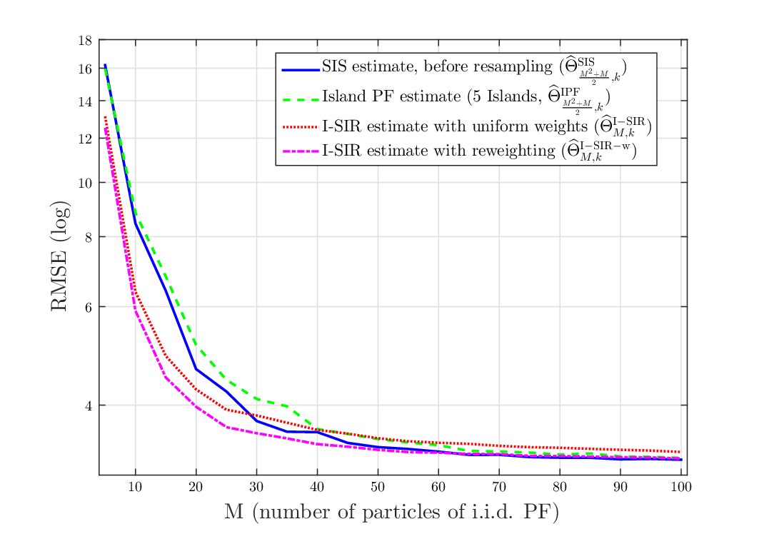
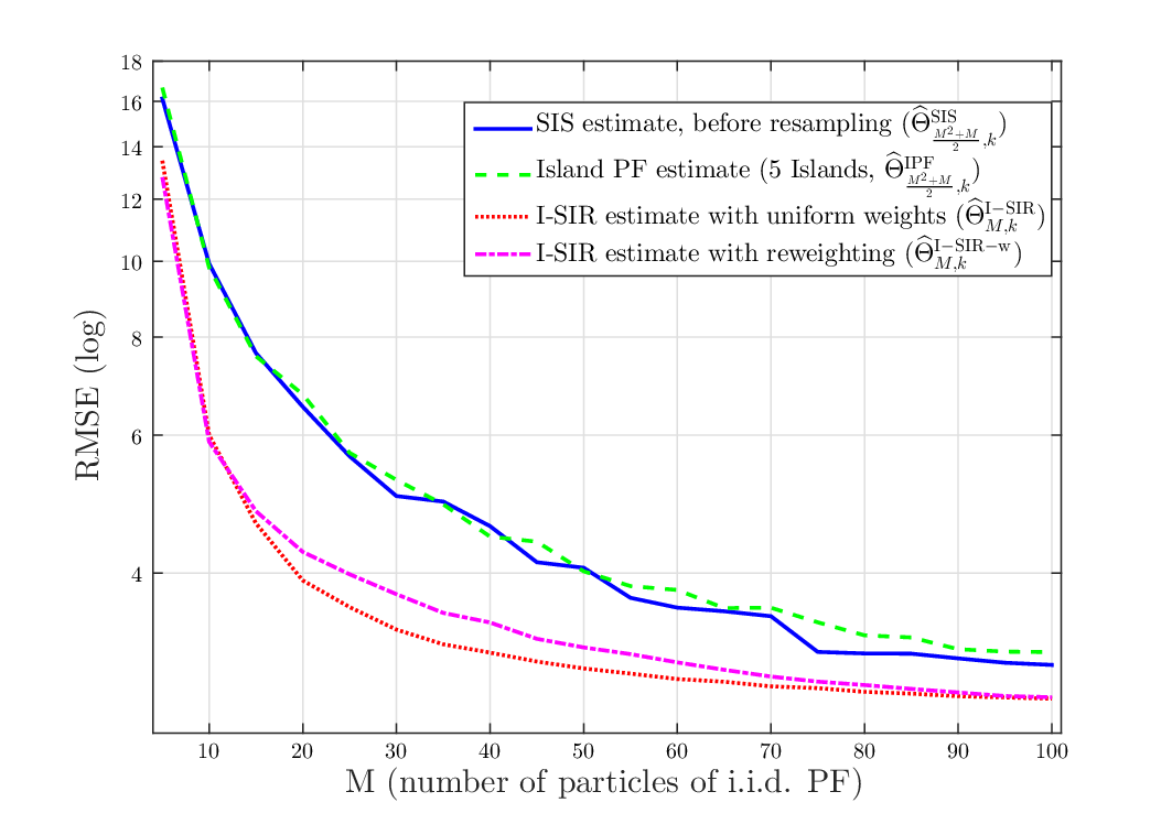
The conditional importance distribution used to sample particles is the transition pdf $q(x_{k}|x_{0:k-1})=f_{k}(x_{k}|x_{k-1})$ ; so the importance weights $w_{k}^{i}$ at time $k$ are proportional to $w_{k-1}^{i}g(y_{k}|x_{k}^{i})$ . We compute $\widehat{\Theta}^{\rm SIS}_{N,k}$ (see (26)), $\widehat{\Theta}^{\rm I-SIR}_{M,k}$ (see (32)), $\widehat{\Theta}^{\rm I-SIR-w}_{M,k}$ (see (40)) with $N=\frac{M^{2}+M}{2}$ to set the number of sampling operations. We also compare these estimates with $\widehat{\Theta}^{\rm IPF}_{N,k}$ deduced from the Island PF with $5$ islands and $N/5$ particles per island.

The results are displayed for two set of parameters. Fig. 3(a) corresponds to the case where $\sigma_{Q}=\sqrt{10}$ , $\sigma_{\rho}=0.25$ and $\sigma_{\theta}=\frac{\pi}{720}$ while Fig 3(b) corresponds to a very informative case where $\sigma_{Q}=\sqrt{10}$ , $\sigma_{\rho}=0.05$ and $\sigma_{\theta}=\frac{\pi}{3600}$ . For the first configuration, we observe that $\widehat{\Theta}^{\rm I-SIR-w}_{M,k}$ outperforms the other estimates and improves $\widehat{\Theta}^{\rm I-SIR}_{M,k}$ which does not rely on weighted samples. Compared to the classical SIS estimate, $\widehat{\Theta}^{\rm I-SIR}_{M,k}$ gives better performance as long as the number of samples $M$ is weak ( $M<30$ , so $N<465$ ) but is next outperformed when the number of samples is large. As shown in Fig. 3(b), when the observations become informative, $\widehat{\Theta}^{\rm I-SIR}_{M,k}$ gives the best performances. Contrary to $\widehat{\Theta}^{\rm SIS}_{N,k}$ and $\widehat{\Theta}^{\rm IPF}_{N,k}$ our estimate does not suffer from the degeneration of the importance weights. Indeed when the measurements are informative (and so the likelihood is sharp), few importance weights have a non null value. However, the independent resampling procedure ensures the diversity of the final samples when we use uniform weights. Concerning $\widehat{\Theta}^{\rm I-SIR-w}_{M,k}$ , remember that it relies on the MC approximation (41). A close analysis of (41) when the likelihood is sharp shows that the final weights tend to be null except that of the particle with the larger likelihood; consequently, in this case the estimate $\widehat{\Theta}^{\rm I-SIR-w}_{M,k}$ is affected by the lack of diversity.

IV-D High dimensional problems

We finally study the impact of the dimension of the hidden state ${X_{k}}$ . We consider a state vector of dimension $m=4\times l$ , $x_{k}=[p_{x,k}^{1},\dot{p}_{x,k}^{1},p_{y,k}^{1},\dot{p}_{y,k}^{1},\cdots,p_{x,k}^{l},\dot{p}_{x,k}^{l},p_{y,k}^{l},\dot{p}_{y,k}^{l}]^{T}$ . Each component $x_{k}^{l}=[p_{x,k}^{l},\dot{p}_{x,k}^{l},p_{y,k}^{l},\dot{p}_{y,k}^{l}]^{T}$ evolves independently from all the other components, according to $f_{k|k-1}(x_{k}|x_{k-1})=\mathcal{N}(x_{k};{\bf F}x_{k-1};{\bf Q})$ where $\tau=1$ ,

\displaystyle\mathbf{F}

\displaystyle=

\displaystyle\begin{pmatrix}1&\tau&0&0\\ 0&1&0&0\\ 0&0&1&\tau\\ 0&0&0&1\end{pmatrix}\text{, }\mathbf{Q}=\sigma^{2}_{Q}\begin{pmatrix}\frac{\tau^{3}}{3}&\frac{\tau^{2}}{2}&0&0\\ \frac{\tau^{2}}{2}&\tau&0&0\\ 0&0&\frac{\tau^{3}}{3}&\frac{\tau^{2}}{2}\\ 0&0&\frac{\tau^{2}}{2}&\tau\\ \end{pmatrix}\text{. }

Each component is observed independently via $g_{k}(y_{k}|x_{k})=\mathcal{N}(y_{k};{\bf H}x_{k};{\bf R})$ where

\displaystyle\mathbf{H}

\displaystyle=

\displaystyle\begin{pmatrix}1&0&0&0\\ 0&0&1&0\\ \end{pmatrix}\text{, }\mathbf{R}=\begin{pmatrix}\sigma_{x}^{2}&0\\ 0&\sigma_{y}^{2}\\ \end{pmatrix}\text{. }

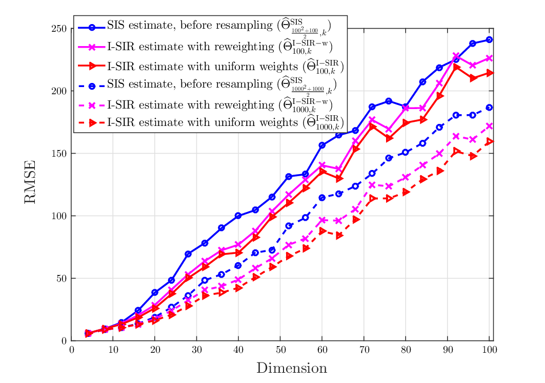
Again, we compute the estimate based on classical PF $\widehat{\Theta}^{\rm SIS}_{N,k}$ (see (26)). It is well known that the PF tends to degenerate when the dimension of the hidden state increases. We also compute $\widehat{\Theta}^{\rm I-SIR}_{M,k}$ (see (32)), $\widehat{\Theta}^{\rm I-SIR-w}_{M,k}$ (see (40)) with $N=\frac{M^{2}+M}{2}$ for $M=100$ and $M=1000$ as a function of the dimension $m$ to see how the dimension impacts our estimate and the classical PF estimate.

The results are displayed in Fig. 4. It can be seen that the estimates $\widehat{\Theta}^{\rm I-SIR}_{M,k}$ and $\widehat{\Theta}^{\rm I-SIR-w}_{M,k}$ outperform $\widehat{\Theta}^{\rm I-SIS}_{M,k}$ more and more significantly as the dimension increases, due to the local impoverishment phenomenon. First, $\widehat{\Theta}^{\rm I-SIR-w}_{M,k}$ outperforms $\widehat{\Theta}^{\rm I-SIR}_{M,k}$ as long as the dimension of the hidden state is low ( $m=4$ and $m=8$ ); when $m$ increases, the estimate based on weighted samples from $\tilde{q}_{N}$ limits the degeneration phenomenon w.r.t. that based on weighted samples from $q$ but using unweighted samples when the dimension is large ensures the diversity and gives better performances. Note that the dependent and independent SIR algorithms give approximately the same performance when $m$ is low but the gap between the dependent and the independent SIR estimates increases with the dimension.

V Conclusion

SMC algorithms in Hidden Markov models are based on the sequential application of the IS principle. However the direct sequential application of the IS principle leads to the degeneration of the weights, against which multinomial resampling has been proposed. This rejunevation scheme, which is now routinely used in SIR algorithms, enables to discard particles (or trajectories) with low weights, but particles with large weights will be resampled several times, which leads to dependency and support degeneracy. In this paper we thus revisited the resampling step used in the classical SIR algorithms. We first addressed the static case, showed that the particles sampled by Rubin’s SIR mechanism are dependent samples drawn from some pdf $\tilde{q}_{N}$ , and proposed an alternative sampling mechanism which produces independent particles drawn from that same marginal pdf $\tilde{q}_{N}$ . This set of independent samples enables us to build a moment estimator which outperforms the classical SIR-based one, both from a non-asymptotical and an asymptotical points of view. Finally the succession of the sampling, weighting and resampling steps indeed transforms an elementary instrumental pdf $q$ into a compound importance distribution $\tilde{q}_{N}=\phi(p,q,N)$ , which leads us to reweight the (originally unweighted) resampled particles $x^{i}$ by post-resampling weights proportional to $\frac{p(x^{i})}{\tilde{q}(x^{i})}$ . Such post-resampling weights cannot be computed exactly, but can easily be estimated by recycling the extra MC samples which were needed for producing the independently resampled particles.

We next adapted this methodology to the dynamic case, in order to estimate a moment of interest in an hidden Markov model. The computation of the post-resampling weights is more challenging than in the static case, but reinterpreting our independent resampling scheme as the first step of a particular APF algorithm enables us to make full use of the APF methodology and so to reweight the final samples via the second-stage APF weights. Finally we validated our discussions by computer-generated experiments and carefully took into account the computational budget. Simulations in model where the FA-APF algorithm is computable show that the independent resampling gives a performance close to the FA-APF algorithm. Consequently, it confirms the relevance of the instrumental mixture pdf used implicitly by the independent resampling PF which can be used in any hidden Markov model since it not require to compute the predictive likelihood nor the optimal importance distribution. Finally independent PF gives very satisfying results when applied in highly informative models which are challenging for classical PF and limits the degeneration phenomenon in high dimensional models.

Proof of Proposition 1

Let $A$ be any Borel set. Let $\mathds{1}_{A}(x)=1$ if $x\in A$ and $0$ otherwise. Then for any $l$ , $1\leq l\leq M_{N}$ ,

		$\displaystyle\Pr(X^{l}\in A)$
		$\displaystyle=\int_{{\rm I\!R}^{N}}[\sum_{i=1}^{N}w^{i}(\tilde{x}^{1},\cdots,\tilde{x}^{N})\mathds{1}_{A}(\tilde{x}^{i})]\prod_{j=1}^{N}q(\tilde{x}^{j}){\rm d}{\tilde{\bf x}}^{1:N}$
		$\displaystyle=\sum_{i=1}^{N}\int_{{\rm I\!R}^{N}}w^{i}(\tilde{x}^{1},\cdots,\tilde{x}^{N})\mathds{1}_{A}(\tilde{x}^{i})\prod_{j=1}^{N}q(\tilde{x}^{j}){\rm d}{\tilde{\bf x}}^{1:N}$
		$\displaystyle=\!\!\sum_{i=1}^{N}\!\int_{A}[\int_{{\rm I\!R}^{N-1}}\!\!\!\!\!\!\!\!\!w^{i}(\tilde{x}^{1},\cdots,\tilde{x}^{N})\prod_{\underset{j\neq i}{j=1}}^{N}q(\tilde{x}^{j}){\rm d}{\tilde{\bf x}}^{1:i-1,i+1:N}]q(\tilde{x}^{i}){\rm d}{\tilde{x}}^{i}$
		$\displaystyle=\sum_{i=1}^{N}\int_{A}h_{N}(\tilde{x}^{i})q(\tilde{x}^{i}){\rm d}{\tilde{x}}^{i}$
		$\displaystyle=\int_{A}Nh_{N}(\tilde{x})q(\tilde{x}){\rm d}{\tilde{x}},$

so $X^{l}$ has pdf $\tilde{q}_{N}$ w.r.t. Lebesque measure.

Proof of Proposition 2

Let $X^{i}$ (for any $i$ , $1\leq i\leq M_{N}$ be produced by the classical SIR mechanism. Then

{\rm E}(f(X^{i}))|\tilde{\bf x}^{1:N})=\widehat{\Theta}^{\rm IS}_{N}.

(44)

So ${\rm E}(\widehat{\Theta}^{\rm SIR}_{M_{N}})|\tilde{\bf x}^{1:N})=\widehat{\Theta}^{\rm IS}_{N},$ and ${\rm E}(\widehat{\Theta}^{\rm SIR}_{M_{N}})=$ ${\rm E}(\widehat{\Theta}^{\rm IS}_{N})$ . On the other hand ${\rm E}(\widehat{\Theta}^{\rm I-SIR}_{M_{N}})=$ ${\rm E}(\widehat{\Theta}^{\rm SIR}_{M_{N}})$ , whence (16). Next

\displaystyle{\rm var}(\widehat{\Theta}^{\rm SIR}_{M_{N}})

\displaystyle=

\displaystyle\frac{1}{M_{N}^{2}}\sum_{i=1}^{M_{N}}{\rm var}(f(X^{i}))+\frac{1}{M_{N}^{2}}\sum_{\stackrel{{\scriptstyle\scriptstyle k,l=1}}{{k\neq l}}}^{M_{N}}\!\!{\rm Cov}(f(X^{k}),f(X^{l})).

(45)

in which $X^{i}\sim\tilde{q}_{N}$ for all $i$ . The first term is equal to ${\rm var}(\widehat{\Theta}^{\rm I-SIR}_{M_{N}})$ . Let us compute the second term. For all $k$ , $l$ , $1\leq k,l,\leq M_{N}$ with $k\neq l$ , ${\rm E}(f(X^{k})f(X^{l})|\tilde{\bf x}^{1:N})=(\widehat{\Theta}^{\rm IS}_{N})^{2},$ so ${\rm E}(f(X^{k})f(X^{l}))={\rm E}({\rm E}(f(X^{k})f(X^{l})|\tilde{\bf X}^{1:N}))={\rm E}((\widehat{\Theta}^{\rm IS}_{N})^{2}).$ Using (44) again, we conclude that ${\rm Cov}(f(X^{k}),f(X^{l}))={\rm var}(\widehat{\Theta}^{\rm IS}_{N}),$ whence (17).

Proof of Theorem 1

We first introduce the following notations:

$\displaystyle\Theta(f)$	$\displaystyle=\int f(x)p(x){\rm d}x\text{,}$	(46)
$\displaystyle\widehat{\Theta}^{\rm IS}_{N}(f)$	$\displaystyle=\sum_{i=1}^{N}\frac{\frac{p(X^{i})}{q(X^{i})}}{\sum_{j=1}^{N}\frac{p(X^{j})}{q(X^{j})}}f(X^{i})\text{, }X^{i}\overset{\rm i.i.d.}{\sim}q(.)\text{,}$	(47)
$\displaystyle\widehat{\Theta}^{\rm I-SIR}_{M_{N}}(f)$	$\displaystyle=\frac{1}{M_{N}}\sum_{i=1}^{M_{N}}f(\overline{X}^{i})\text{, }\overline{X}^{i}\overset{\rm i.i.d.}{\sim}\tilde{q}_{N}(.)\text{,}$	(48)

and we will assume that ${\rm E}(\widehat{\Theta}^{\rm IS}_{N}(f^{2}))$ is finite.

Using ${\rm E}(\Theta^{\rm I-SIR}_{M_{N}}(f))={\rm E}(\Theta^{\rm IS}_{N}(f))$ , we have

		$\displaystyle\sqrt{M_{N}}\left(\widehat{\Theta}^{\rm I-SIR}(f)-\Theta(f)\right)=A_{N}+B_{N}\text{,}$		(49)
		$\displaystyle A_{N}=\sqrt{M_{N}}(\widehat{\Theta}^{\rm I-SIR}(f)-{\rm E}(\widehat{\Theta}^{\rm I-SIR}(f)))\text{,}$		(50)
		$\displaystyle B_{N}=\frac{\sqrt{M_{N}}}{\sqrt{N}}{\rm E}(\sqrt{N}(\widehat{\Theta}^{\rm IS}_{N}(f)-\Theta(f)))\text{.}$		(51)

Our objective is to show that $A_{N}$ converges to a centered Gaussian distribution with variance ${\rm var}_{p}(f(X))$ and that $B_{N}$ converges to $0$ .

Convergence of $B_{N}$

We have recalled (see (9)) that under mild assumptions [4]

\sqrt{N}(\widehat{\Theta}^{\rm IS}_{N}(f)-\Theta(f))\overset{\mathcal{D}}{\rightarrow}\mathcal{N}\left(0,{\rm E}_{q}\left(\frac{p^{2}(X)}{q^{2}(X)}(f(X)-\Theta)^{2}\right)\right)\text{.}

According to Theorem 9.1.10 in [14], ${\rm E}(|\sqrt{N}(\widehat{\Theta}^{\rm IS}_{N}(f)-\Theta(f))|^{2})$ is bounded and so its upper bound is finite. According to the corollary of Theorem 25.12 in [29], it is ensured that $\sqrt{N}{\rm E}((\widehat{\Theta}^{\rm IS}_{N}(f)-\Theta(f)))\rightarrow 0$ ; consequently

\frac{\sqrt{M_{N}}}{\sqrt{N}}{\rm E}(\sqrt{N}(\widehat{\Theta}^{\rm IS}_{N}(f)-\Theta(f)))\rightarrow 0\text{.}

(52)

Convergence of $A_{N}$

$A_{N}$ reads

\sqrt{M_{N}}\left(\frac{1}{M_{N}}\sum_{i=1}^{M_{N}}f(\overline{X}^{i})-{\rm E}(f(\overline{X}^{i}))\right)\text{.}

(53)

To prove the convergence when $N\rightarrow\infty$ , we need a CLT for triangular arrays and we use the version presented in Theorem 9.5.13 of [14]. The required assumptions are:

1.

$\{\overline{X}^{i}\}_{i=1}^{M_{N}}$ are independent;
2.

$\frac{1}{M_{N}}\sum_{i=1}^{M_{N}}{\rm E}(f^{2}(\overline{X}^{i}))-({\rm E}(f(\overline{X}^{i})))^{2}\rightarrow{\rm var}_{p}(f(X))$ ;
3.

for any positive $C$ , $\frac{1}{M_{N}}\sum_{i=1}^{M_{N}}{\rm E}(f^{2}(\overline{X}^{i})\mathds{1}_{|f(\overline{X}^{i})|\geq C})\rightarrow\Theta(f^{2}\mathds{1}_{|f|\geq C})$ .

Assumption 1) is satisfied since $\{\overline{X}^{i}\}_{i=1}^{M_{N}}$ are i.i.d. from $\tilde{q}_{N}$ . Next, ${\rm E}(f(\overline{X}^{i}))={\rm E}_{\tilde{q}_{N}}(f(\overline{X}))$ which coincides with ${\rm E}(\widehat{\Theta}^{\rm IS}_{N}(f))$ . Using again Theorem 9.1.10 of [14] and Theorem 25.12 of [29], ${\rm E}(\widehat{\Theta}^{\rm IS}_{N}(f))\rightarrow\Theta(f)$ when $N\rightarrow\infty$ . With the same argument, ${\rm E}(f^{2}(\overline{X}^{i}))\rightarrow\Theta(f^{2})$ . Consequently, assumption 2) is satisfied since

\displaystyle\frac{1}{M_{N}}\sum_{i=1}^{M_{N}}{\rm E}(f^{2}(\overline{X}^{i}))-({\rm E}(f(\overline{X}^{i})))^{2}={\rm E}_{\tilde{q}_{N}}(f^{2}(\overline{X}))-({\rm E}_{\tilde{q}_{N}}(f(\overline{X})))^{2}\rightarrow\Theta(f^{2})-(\Theta(f))^{2}={\rm var}_{p}(f(X)).

Finally, ${\rm E}(f^{2}(\overline{X}^{i})\mathds{1}_{|f(\overline{X}^{i})|\geq C})={\rm E}(\widehat{\Theta}^{\rm IS}_{N}(f^{2}\mathds{1}_{|f|\geq C}))$ which converges to $\Theta(f^{2}\mathds{1}_{|f|\geq C})$ and assumption 3) is satisfied. Consequently,

\sqrt{M_{N}}(\frac{1}{M_{N}}\sum_{i=1}^{M_{N}}f(\overline{X}^{i})-{\rm E}(f(\overline{X}^{i})))\overset{\mathcal{D}}{\rightarrow}\mathcal{N}(0,{\rm var}_{p}(f(X)))\text{.}

(54)

Combining (52), (54) and (49) we obtain (18).

References

[1] N. J. Gordon, D. J. Salmond, and A. F. M. Smith, “Novel approach to nonlinear/ non-Gaussian Bayesian state estimation,” IEE Proceedings-F, vol. 140, no. 2, pp. 107–113, April 1993.
[2] A. Doucet, N. de Freitas, and N. Gordon, Eds., Sequential Monte Carlo Methods in Practice, ser. Statistics for Engineering and Information Science. New York: Springer Verlag, 2001.
[3] M. Arulampalam, S. Maskell, N. Gordon, and T. Clapp, “A tutorial on particle filters for online nonlinear / non-Gaussian Bayesian tracking,” IEEE Transactions on Signal Processing, vol. 50, no. 2, pp. 174–188, February 2002.
[4] J. Gewecke, “Bayesian inference in econometric models using Monte Carlo integration,” Econometrica, vol. 57, no. 6, pp. 1317–1339, November 1989.
[5] A. Kong, J. S. Liu, and W. H. Wong, “Sequential imputations and bayesian missing data problems,” Journal of the American Statistical Association, vol. 89, no. 425, pp. 278–88, March 1994.
[6] J. S. Liu and R. Chen, “Blind deconvolution via sequential imputation,” Journal of the American Statistical Association, vol. 90, no. 430, pp. 567–76, June 1995.
[7] J. S. Liu, “Metropolized independent sampling with comparisons to rejection sampling and importance sampling,” Statistics and Computing, vol. 6, pp. 113–119, 1996.
[8] J. Cornebise, É. Moulines, and J. Olsson, “Adaptive methods for sequential importance sampling with application to state-space models,” Statistics and Computing, vol. 18, no. 4, pp. 461–480, 2008.
[9] A. F. M. Smith and A. E. Gelfand, “Bayesian statistics without tears : a sampling-resampling perspective.” The American Statistician, vol. 46, no. 2, pp. 84–87, 1992.
[10] R. Douc, O. Cappé, and É. Moulines, “Comparison of resampling schemes for particle filtering,” in Proceedings of the 4th International Symposium on Image and Signal Processing and Analysis (ISPA), Zagreb, Croatia, September 2005.
[11] T. Li, M. Bolić, and P. M. Djuric, “Resampling Methods for Particle Filtering: Classification, implementation, and strategies,” IEEE Signal Processing Magazine, vol. 32, no. 3, pp. 70–86, May 2015.
[12] D. B. Rubin, “Using the SIR algorithm to simulate posterior distributions,” in Bayesian Statistics III, M. H. Bernardo, K. M. Degroot, D. V. Lindley, and A. F. M. Smith, Eds. Oxford: Oxford University Press, 1988.
[13] A. E. Gelfand and A. F. M. Smith, “Sampling based approaches to calculating marginal densities,” Journal of the American Statistical Association, vol. 85, no. 410, pp. 398–409, 1990.
[14] O. Cappé, É. Moulines, and T. Rydén, Inference in Hidden Markov Models. Springer-Verlag, 2005.
[15] Y. Petetin and F. Desbouvries, “Optimal SIR algorithm vs. fully adapted auxiliary particle filter: a non asymptotical analysis,” Statistics and computing, vol. 23, no. 6, pp. 759–775, 2013.
[16] T. Hesterberg, “Advances in importance sampling,” Ph.D. dissertation, Stanford University, 1988.
[17] P. del Moral, Feynman-Kac formulae. Genealogical and interacting particle systems with applications, ser. Probability and its applications. New-York: Springer, 2004.
[18] J. S. Liu, Monte Carlo strategies in scientific computing. Springer, 2001.
[19] A. Doucet, S. J. Godsill, and C. Andrieu, “On sequential Monte Carlo sampling methods for Bayesian filtering,” Statistics and Computing, vol. 10, pp. 197–208, 2000.
[20] R. van der Merwe, A. Doucet, N. de Freitas, and E. Wan, “The Unscented Particle Filter.” Advances in Neural Information Processing Systems, 2000.
[21] S. Saha, P. K. Manda, Y. Boers, H. Driessen, and A. Bagchi, “Gaussian proposal density using moment matching in SMC methods.” Statistics and Computing, vol. 19, no. 2, pp. 203–208, 2009.
[22] D. Crisan and A. Doucet, “A survey of convergence results on particle filtering methods for practitioners,” IEEE Transactions on Signal Processing, vol. 50, no. 3, pp. 736–46, March 2002.
[23] N. Chopin, “Central limit theorem for sequential Monte Carlo methods and its application to Bayesian inference,” The Annals of Statistics, vol. 32, no. 6, pp. 2385–2411, 2004.
[24] C. Vergé, C. Dubarry, P. Del Moral, and É. Moulines, “On parallel implementation of sequential monte carlo methods: the island particle model,” Statistics and Computing, vol. 25, no. 2, pp. 243–260, 2015. [Online]. Available: http://dx.doi.org/10.1007/s11222-013-9429-x
[25] M. K. Pitt and N. Shephard, “Filtering via simulation : Auxiliary particle filter,” Journal of the American Statistical Association, vol. 94, no. 446, pp. 590–99, June 1999.
[26] A. M. Johansen and A. Doucet, “A note on the auxiliary particle filter,” Statistics and Probability Letters, vol. 78, no. 12, pp. 1498–1504, September 2008.
[27] N. Whiteley and A. M. Johansen, “Recent developments in auxiliary particle filtering,” in Inference and Learning in Dynamic Models, Barber, Cemgil, and Chiappa, Eds. Cambridge University Press, 2010.
[28] R. Douc, É. Moulines, and J. Olsson, “Optimality of the auxiliary particle filter,” Probability and Mathematical Statistics, vol. 29, no. 1, pp. 1–28, 2009.
[29] P. Billingsley, Probability and Measure, ser. Wiley Series in Probability and Statistics. Wiley, 1995. [Online]. Available: https://books.google.de/books?id=z39jQgAACAAJ

	$\displaystyle{\rm E}(\widehat{\Theta}_{N,k}^{\rm I-SIR}\|\{x_{0:k-1}^{i}\}_{i=1}^{N})$	$\displaystyle={\rm E}(\widehat{\Theta}_{n}^{\rm SIR}\|\{x_{0:k-1}^{i}\}_{i=1}^{N})\text{,}$		(33)
	$\displaystyle{\rm var}(\widehat{\Theta}_{N,k}^{\rm SIR}\|\{x_{0:k-1}^{i}\}_{i=1}^{N})$	$\displaystyle={\rm var}(\widehat{\Theta}_{n}^{\rm I-SIR}\|\{x_{0:k-1}^{i}\}_{i=1}^{N})+\frac{N-1}{N}{\rm var}(\widehat{\Theta}_{N,k}^{\rm SIS}\|\{x_{0:k-1}^{i}\}_{i=1}^{N})\text{.}$		(34)

Independent Resampling Sequential Monte Carlo Algorithms

Abstract

Index Terms:

I Introduction

II IS with resampling viewed as a compound IS scheme

II-A The dependent SIR mechanism

II-A1 Properties of the sampled particles {x~i}i=1N\{\tilde{x}^{i}\}_{i=1}^{N}

II-A2 Properties of the resampled particles {xi}i=1MN\{x^{i}\}_{i=1}^{M_{N}}

Proposition 1

II-B The independent SIR mechanism

II-B1 Statistical properties

Proposition 2

Theorem 1

II-B2 Sampling procedure

II-C Reweighting the independent samples?

II-D Summary

III Independent resampling based PF

III-A Classical SIR algorithms (based on dependent resampling)

III-B An alternative SIR algorithm (based on independent resampling)

Proposition 3

Remark 1

III-C Interpretation of the independent sampling scheme in terms of APF

III-C1 A brief presentation of APF

III-C2 Independent resampling as the first step of a canonical APF algorithm

III-C3 Reweighting the independent samples?

III-D Summary

IV Simulations

IV-A Comparison of static sampling procedures

IV-B Comparison with APF algorithms

IV-C Tracking from range-bearing measurements

IV-D High dimensional problems

V Conclusion

Proof of Proposition 1

Proof of Proposition 2

Proof of Theorem 1

Convergence of BNB_{N}

Convergence of ANA_{N}

References

II-A1 Properties of the sampled particles $\{\tilde{x}^{i}\}_{i=1}^{N}$

II-A2 Properties of the resampled particles $\{x^{i}\}_{i=1}^{M_{N}}$

Convergence of $B_{N}$

Convergence of $A_{N}$