∎
Generalized model for anisotropic compact stars
Abstract
In the present investigation an exact generalized model for anisotropic compact stars of embedding class one is sought for under general relativistic background. The generic solutions are verified by exploring different physical aspects, viz. energy conditions, mass-radius relation, stability of the models, in connection to their validity. It is observed that the model present here for compact stars is compatible with all these physical tests and thus physically acceptable as far as the compact star candidates , and are concerned.
Keywords:
general relativity; embedding class one; anisotropic fluid; compact stars1 Introduction
The studies on anisotropic compact stars remain always a topic of great interest in the relativistic astrophysics. The detailed works of several scientists [1, 2, 3, 4, 5] make our understanding clear about the highly dense spherically symmetric fluid spheres having pressure anisotropic in nature. Usually anisotropy arises due to presence of mixture of fluids of different types, rotation, existence of superfulid, presence of magnetic field or external field and phase transition etc. According to Ruderman [2] for the high density anisotropy is the inherent nature of nuclear matters and their interactions are relativistic. In this connection some other works on the anisotropic compact star models can be looked in to the following Refs. [6, 7, 8, 9, 10, 11, 12, 13].
Recent study by Randall-Sundram and Anchordoqui-Bergliaffa [14, 15] re-establishes the idea that our 4-dimensional spacetime is embedded in higher dimensional flat space as predicted earlier by Eddington [16]. It is known that the manifold can be embedded in pseudo-Euclidean space of dimensions. The class of manifold which is less than or equal to can be defined as the minimum extra dimension () of the pseudo-Euclidean space required for embedding in . It is to note that when , i.e. for the relativistic spacetime , the corresponding value of relativistic embedding class is 6. The values of the same for the plane and spherical symmetric spacetime are respectively 3 and 2. The class of Kerr is 5 [17] whereas the class of Schwarzschild’s interior and exterior solutions are respectively 2 and 1 and the same for the Friedman-Robertson-Lemaître spacetime [18] is 1. In some of our previous works [19, 20, 21, 22] we have successfully discussed different stellar models under the embedding class 1.
In this paper utilizing embedding class 1 metric we have attempted to study an anisotropic spherically symmetric stellar model. In this investigation we have assumed that the metric potential , where . The reasons for the choice of are as follows:
(i) with the choice of the space-time becomes flat;
(ii) with the choice of this becomes the famous Kohlar-Chao solution [23];
(iii) with the choice of , as velocity of sound is not decreasing so we will get a solution which is not well behaved.
We have, therefore, studied our proposed model varying to and discussed the physical properties of the system for these values of . In the later part one may find from Table 1 that for , the product becomes almost a constant, say . This situation shows that for large values of (say infinity) we obtain , which is the same metric potential ( with ) as considered by Maurya et al. [19, 24].
Under the above background the outline of the present work is as follows: we provide the Einstein field equations and their solutions in Sect. 2. In the next Sect. 3 the boundary conditions are discussed to find out constants of integration. The Sec. 4 deals with the applications of the solutions to check several physical properties of the model regarding validity with the stellar structure. Some remarks are passed in concluding Sect. 5.
2 Basic field equations and solutions
To describe the interior of a static and spherically symmetry object the line element in the Schwarzschild co-ordinate can be written as
| (1) |
where and are the functions of the radial coordinate .
Now if the spacetime Eq. (1) satisfies the Karmarkar condition [25]
| (2) |
with [26], it represents the spacetime of emending class .
For the condition (2), the line element Eq. (1) gives the following differential equation
| (3) |
with .
Solving Eq. (3) we get
| (4) |
where is an arbitrary integrating constant.
We are assuming that within the star the matter is anisotropic and the corresponding energy-momentum tensor can be taken in the form
| (5) |
with and , the vector being the fluid 4-velocity and is the space-like vector which is orthogonal to . Here is the matter density, is the the radial and is transverse pressure of the fluid in the orthogonal direction to .
Assuming with (in relativistic geometrized unit) the Einstein field equations are given by
| (6) |
| (7) |
| (8) |
Here we have four equations with five unknowns, namely and which are to be find out under the proposed model. This immediately prompt us to explore for some suitable relationship between the unknowns or an existing physically acceptable metric potential can be opted for which will help us to overcome the mathematical situation of redundancy.
Therefore, to solve the above set of Einstein field equations let us take the metric co-efficient, , as proposed by Lake [27]
| (9) |
where and are constants and .

Solving Eqs. (4) and (9) we obtain
| (10) |
where

| (12) |
| (13) |


and the anisotropic factor is obtained as
| (14) |
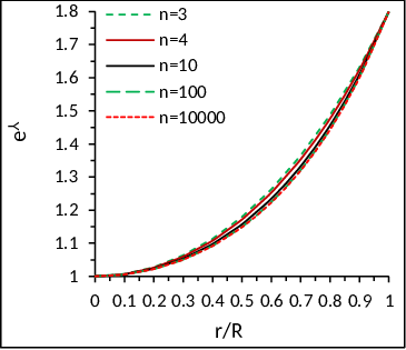
where . The profiles of the metric functions, effective density, the effective radial and tangential pressures, the anisotropic factor are respectively shown in Figs. 1-4.
From Fig. 4 we also find that for our system the anisotropic factor is minimum at the centre and it is maximum at the surface as proposed by Deb et al. [28] for the anisotropic stellar model. However the anisotropy factor is zero for all radial distance if and only if . This implies that in the absence of anisotropy the radial and transverse pressures and density become zero. Also in this case the metric turns out to be flat.

3 Boundary conditions to determine the constants
For fixing the values of the constants, we match our interior space-time to the exterior Schwarzschild line element given by
| (15) |
Outside the event horizon , being the mass of the black hole. Also the radial pressure must be finite and positive at the centre of the star which must vanish at the surface [29]. Then = 0 gives:
| (16) |
This yields the radius of star as
| (17) |
using the continuity of the metric coefficient and (matching of second fundamental form at is same as radial pressure should be zero at ) across the boundary we get the following three equations
| (18) |
| (19) |
| (20) |
Solving Eq. (16) and Eqs. (18)-(20), in terms of mass of radius of the compact star, we obtained the expressions for , and as
| (21) |
| (22) |
| (23) |
However, the value of arbitrary constant is determined by using the density of star at the surface, i.e. as
| (24) |
The gradients of density and radial pressure (by taking ) as
| (25) |
| (26) |
where
,
, .
4 Physical features of the anisotropic models
In this section different physical features of the compact stars will be discussed.
4.1 Energy Conditions
To satisfy energy conditions i.e null energy condition (NEC), weak energy condition (WEC) and strong energy condition (SEC) the anisotropic fluid spheres must be consistent with the following inequalities simultaneously inside the stars given as
| (27) |
| (28) |
| (29) |
From Fig. 5 it is clear that the energy conditions are satisfied in the interior of the compact stars simultaneously.


4.2 Mass-radius relation
For the physical validity of the model according to Buchdahl [30] the mass to radius ratio for perfect fluid should be which was later proposed in a more generalized expression by Mak and Harko [6].
The Effective mass of the compact star is obtained as
| (30) |
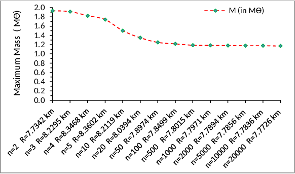
In Fig. 6 variation of maximum mass with respect to corresponding radius of the compact stars with the different values of have shown. We have also plotted in Fig. 7 variation of maximum values of for the different values of . We found throughout the study for the different values of n our system is valid with the Buchdahl conditions [30] which is also clear from Fig. 7.

The compactification factor of the stars is obtained as
| (31) |
The surface redshift with respect to the above compactness (u) is given as
| (32) |
whose behaviour is shown in Fig. 8 with the fractional coordinate for .

4.3 Stability of the model
In the following sub sections we will try to study the stability of the proposed mathematical model.
4.3.1 Generalized TOV equation
Following Tolman [31], Oppenheimer and Volkoff [32] we want to examine whether our present model is stable under the three forces, viz. gravitational force (), hydrostatics force () and anisotropic force () so that the sum of the forces becomes zero for the system to be in equilibrium, i.e.
| (33) |
The generalized TolmanOppenheimerVolkoff (TOV) equation [33, 8] for our system takes form as following
| (34) |
where represents the gravitational mass within the radius , which can derived from the Tolman-Whittaker formula [34] and the Einstein field equations and is defined by
| (35) |
Plugging the value of in equation , we get
| (36) |
| (38) |
| (39) |
where, and . We have shown the behaviour of TOV equation with in Fig. 9 for . As far as equilibrium is concerned the plots are satisfactory in their nature.


.
4.3.2 Herrera’s cracking concept
With the help of Herrera’s [35] ‘cracking concept’ we try to examine the stability of the proposed configuration. For physical validity the fluid distribution must admit the condition of causality which suggests that square of radial and tangential sound speeds individually must lie within the limit 0 and 1. Also following Herrera [35] and Abreu et al. [36] it can be concluded that for the stable region provided condition is which indicates that for the stable region ‘no cracking’ is the another essential condition. For our system sound velocities are
| (40) |
| (41) |


where
;
;
;
;
.
From Figs. 10-11 it is clear that our stellar system satisfies all the conditions said above and hence provides a stable configuration.
4.3.3 Adiabetic index
According to Heintzmann and Hillebrandt [37] the required condition for the stability of the isotropic compact stars is the adiabatic index, in the all interior points of the stars. For our model we have
| (42) |
| (43) |
where
, .


From Fig. 12 it is obvious that for all the values of are greater than and hence our system is stable.
5 Discussions and conclusions
In the present paper we have performed certain investigations on the nature of compact stars by utilizing embedding class one metric. Here an anisotropic spherically symmetric stellar model has been considered. To carried out the investigations we have considered the following assumptions that the metric , where . The reasons for such consideration on are already have mentioned in the introductory part and are as follows: (i) with the choice of the spacetime becomes flat as Minkowski type; (ii) with the choice of this becomes the famous Kohlar-Chao solution [23] and (iii) with the choice of , the spacetime does not provide well behaved solutions.
Under the above circumstances, therefore, we have studied our proposed model for variation of to . We find from Table 1 that for , the product becomes almost a constant (say ). Thus we can conclude that for the large values of (say infinity) we have the metric potential as considered by Maurya et al. [19, 24] in their previous literature. This result therefore helps us in turn to explore behaviour of the mass and radius of the spherical stellar system as can be observed from Fig. 6. We have shown here variation of maximum mass (in km) with respect to corresponding radius (in km) for different value of . The profile is very indicative which shows that up to and km maximum mass feature is roughly steady and after it gradually decreases. However, after and km the maximum mass again acquires almost a steady feature. In Fig. 7 the Buchdahl condition, i.e. mass-radius relation regarding stable configuration of the stellar system has been shown to be satisfactorily followed.
The main features of the present work therefore can be highlighted for the nature of compact stars as follows:
(1) The stars are anisotropic in their configurations unless . The radial pressure vanishes but tangential pressure does not vanish at the boundary (radius of the star). However, the radial pressure is equal to the tangential pressure at the centre of the fluid sphere. The anisotropy factor is zero for all radial distance if and only if . This implies that in the absence of anisotropy the radial and transverse pressures and density become zero. Also the metric turns out to be flat.
(2) To solve the Einstein field equations we consider the metric co-efficient, as proposed by Lake [27] and hence the spacetime of the interior of the compact stars can be described by Lake metric.
(3) We observe from Fig. 4 that for our system the anisotropic factor is minimum at the centre and maximum at the surface as proposed by Deb et al. [28]. However, the anisotropy factor is zero for all radial distance if and only if . This implies that in the absence of anisotropy the pressures and density become zero which in turn makes the metric to be flat.
(4) The energy conditions are fulfilled as can be seen from Fig. 5 under variation of .
(5) We have discussed about the stability of the model by applying (i) the TOV equation, (ii) the Herrera cracking concept, and (iii) the adiabatic index of the interior of the star. It can be observed that stability of the model has been attained surprisingly in our model (see Figs. 9-11).
(6) The surface redshift analysis for our case shows that for the compact star this turns out to be as maximum value. In the isotropic case and in the absence of the cosmological constant it has been shown that [30, 38, 39] whereas Böhmer and Harko [39] argued that for an anisotropic star in the presence of a cosmological constant the surface redshift must obey the general restriction , which is consistent with the bound as obtained by Ivanov [5]. Therefore, for an anisotropic star without cosmological constant our present value seems to be satisfactory. It is to further note that this low value surface redshift is not at unavailable in the literature where Shee et al. [40] obtained a numerical value for as (also see following Refs. [12, 41, 42, 43, 44] for low valued surface redshift).
| 0.0128 | 0.1535 | 0.0043 | 0.3623 | 81.0930 | 4.5094 | |
| 0.0123 | 0.1109 | 0.0031 | 0.3651 | 81.0968 | 5.8353 | |
| 0.0115 | 0.04158 | 0.0012 | 0.3700 | 81.0905 | 13.8611 | |
| 0.0111 | 0.004009 | 1.1136 | 0.3727 | 81.0794 | 134.5882 | |
| 0.0111 | 3.9950 | 1.1095 | 0.3729 | 81.0877 | 1.3420 | |
| 0.0111 | 3.9920 | 1.1089 | 0.3730 | 81.0930 | 1.3418 |
| Compact stars | |||||||
|---|---|---|---|---|---|---|---|
| RXJ 1856-37 | 0.9042 | 6.002 | 0.1535 | 0.1109 | 0.04158 | 0.004009 | 3.9920 |
| SAX J1808.4- 3658(SS2) | 1.3238 | 6.35 | 0.3610 | 0.2484 | 0.08643 | 0.00802 | |
| SAX J1808.4- 3658(SS1) | 1.4349 | 7.07 | 0.3295 | 0.2283 | 0.0803 | 0.00749 |
| value | Central Density | Surface density | Central pressure |
|---|---|---|---|
| of | |||
| 3.0973 | 1.4966 | 3.0722 | |
| 2.8952 | 1.5455 | 3.2227 | |
| 2.5791 | 1.6339 | 3.4275 | |
| 2.4145 | 1.6870 | 3.5212 | |
| 2.3987 | 1.6921 | 3.5294 | |
| 2.3969 | 1.6926 | 3.5283 |
(7) In Table 2 and 3 we have calculated the central density, surface density and central pressure as well as mass and radius of different compact stars. It is interesting to note that all the data are fall within the observed range of the corresponding star’s physical parameters [12, 41, 42, 43, 44, 45, 28]. It would be interesting to perform a comparative study with the data of our Table 3 with that of Table 4 of Deb et al. [28] where they have prepared the table for the value of only for different compact stars whereas in the present study our table includes a wide range of to . Thus, the Table 3 describes behaviour of certain physical parameters for varying . It is observed that the central density decreases with increasing unlike the surface density which behaves oppositely. However, the central pressure increases with increasing .
The overall observation is that our proposed model satisfies all physical requirements. The entire analysis has been performed in connection to direct comparison of some of the compact star candidates, e.g. , and which confirms validity of the present model.
Acknowledgments
SKM acknowledges support from the authority of University of Nizwa, Nizwa, Sultanate of Oman. SR is thankful to the Inter-University Centre for Astronomy and Astrophysics (IUCAA), Pune, India for providing Visiting Associateship under which a part of this work was carried out. SR is also thankful to the authority of The Institute of Mathematical Sciences, Chennai, India for providing all types of working facility and hospitality under the Associateship scheme.
References
- (1) R.L. Bowers, E. P. T. Liang, Class. Astrophys. J. 188, 657 (1974).
- (2) R. Ruderman, Class. Ann. Rev. Astron. Astrophys. 10, 427 (1972).
- (3) F.E. Schunck, E.W. Mielke, Class. Quantum Gravit. 20, 301 (2003).
- (4) L. Herrera, N.O. Santos, Phys. Report. 286, 53 (1997).
- (5) B.V. Ivanov, Phys. Rev. D 65, 104011 (2002).
- (6) M.K. Mak, T. Harko, Proc. R. Soc. A 459, 393 (2003).
- (7) V.V. Usov, Phys. Rev. D 70, 067301 (2004).
- (8) V. Varela, F. Rahaman, S. Ray, K. Chakraborty, M. Kalam, Phys. Rev. D 82, 044052 (2010).
- (9) F. Rahaman, S. Ray, A. K. Jafry, K. Chakraborty, Phys. Rev. D 82, 104055 (2010).
- (10) F. Rahaman, P.K.F. Kuhfittig, M. Kalam, A.A. Usmani, S. Ray, Class. Quantum Gravit. 28, 155021 (2011).
- (11) F. Rahaman, R. Maulick , A.K. Yadav, S. Ray, R. Sharma, Gen. Relativ. Gravit. 44,107 (2012).
- (12) M. Kalam, F. Rahaman, S. Ray, Sk. Monowar Hossein, I. Karar, J. Naskar, Eur. Phys. J. C 72, 2248 (2012).
- (13) D. Deb, S.R. Chowdhury, S. Ray, F. Rahaman, arXiv:1509.00401 [gr-qc]
- (14) L. Randall, R. Sundram, Phys. Rev. Lett. 83, 3370 (1999).
- (15) L. Anchordoqui, S.E.P. Bergliaffa, Phys. Rev. D 62, 067502 (2000)
- (16) A.S. Eddington, The Mathematical Theory of Relativity, Cambridge University Press, Cambridge (1924).
- (17) R.R. Kuzeev, Gravit. Teor. Otnosit. 16, 93 (1980).
- (18) H.P. Robertson, Rev. Mod. Phys. 5, 62 (1933).
- (19) S.K. Maurya, Y.K. Gupta, B. Dayanandan, S. Ray, Eur. Phys. J. C 76 266 (2016).
- (20) S.K. Maurya, Y.K. Gupta, S. Ray, B. Dayanandan, Eur. Phys. J. C 75 225 (2016).
- (21) S.K. Maurya, Y.K. Gupta, S. Ray, V. Chatterjee, arXiv:1507.01862 [gr-qc]
- (22) S.K. Maurya, Y.K. Gupta, S. Ray, D. Deb, arXiv:1605.01268v2 [gr-qc]
- (23) M. Kohler, K.L. Chao, Z. Naturforsch. Ser. A 20, 1537 (1965).
- (24) S.K. Maurya, Y.K. Gupta, S. Ray, S. Roy Chowdhury, Eur. Phys. J. C 75 389 (2015).
- (25) K.R. Karmarkar, Proc. Ind. Acad. Sci. A 27, 56 (1948).
- (26) S.N. Pandey, S.P. Sharma, Gen. Relativ. Gravit. 14, 113 (1982).
- (27) K. Lake, Phys. Rev. D 67, 104015 (2003).
- (28) D. Deb, S.R. Chowdhury, S. Ray, F. Rahaman, B.K. Guha, arXiv:1606.00713 (2016).
- (29) C.W. Misner, D.H. Sharp, Phys. Rev. B 136, 571 (1964).
- (30) H.A. Buchdahl, Phys. Rev. D 116, 1027 (1959).
- (31) R.C. Tolman, Phys. Rev. 55, 364 (1939).
- (32) J.R. Oppenheimer, G.M. Volkoff, Phys. Rev. 55, 374 (1939).
- (33) J. Ponce de León, Gen. Relativ. Gravit. 25, 1123 (1993).
- (34) J. Devitt, P.S. Florides, Gen. Relativ. Gravit. 21, 585 (1989).
- (35) L. Herrera, Phys. Lett. A 165, 206 (1992).
- (36) H. Abreu, H. Hernandez, L.A. Nunez, Class. Quantum Gravit. 24, 4631 (2007).
- (37) H. Heintzmann, W. Hillebrandt, Astron. Astrophys. 38, 51 (1975).
- (38) N. Straumann, General Relativity and Relativistic Astrophysics, Springer Verlag, Berlin (1984).
- (39) C.G. Böhmer, T. Harko, Class. Quantum Gravit. 23, 6479 (2006).
- (40) D. Shee, F. Rahaman, B.K. Guha, S. Ray, Astrophys. Space Sci. 361, 167 (2016).
- (41) F. Rahaman, R. Sharma, S. Ray, R. Maulick, I. Karar, Eur. Phys. J. C 72, 2071 (2012).
- (42) Sk M. Hossein, F. Rahaman, J. Naskar, M. Kalam, S. Ray, Int. J. Mod. Phys. D 21, 1250088 (2012).
- (43) M. Kalam, A.A. Usmani, F. Rahaman, S.M. Hossein, I. Karar, R. Sharma, Int. J. Theor. Phys. 52, 3319 (2013).
- (44) P. Bhar, F. Rahaman, S. Ray, V. Chatterjee, Eur. Phys. J. C 75, 190 (2015).
- (45) S.K. Maurya, Y.K.Gupta, B. Dayanandan, S. Ray, Eur. Phys. J. C 76, 266 (2016).