Transmission and tunneling probability in two-band metals: influence of magnetic breakdown on the Onsager phase of quantum oscillations
Abstract
Tunneling amplitude through magnetic breakdown (MB) gap is considered for two bands Fermi surfaces illustrated in many organic metals. In particular, the S-matrix associated to the wave-function transmission through the MB gap for the relevant class of differential equations is the main object allowing the determination of tunneling probabilities and phases. The calculated transmission coefficients include a field-dependent Onsager phase. As a result, quantum oscillations are not periodic in for finite magnetic breakdown gap. Exact and approximate methods are proposed for computing ratio amplitudes of the wave-function in interacting two-band models.
August 24, 2026
1 Introduction
In recent years, interest regarding determination of the quantum oscillations phase has been renewed. This was in particular motivated by the observation of a Berry phase both in three-dimensional metals [1] and topological insulators [2], for example in the case of Dirac fermions [3]. One might add the effect of non-parabolicity of the dispersion equation which, both in conventional fermions and, especially, in Dirac fermions is liable to induce phase offsets [4].
The problem of the Onsager phase was nevertheless addressed much earlier, regarding the effect of the phase offset induced by magnetic breakdown (MB) [5, 6, 7]. The case of the model Fermi surface (FS), known as the linear chain of coupled orbits by Pippard [8], is addressed in Refs. [5, 6]. As it is well known, the first experimental realization of this FS topology was observed in the organic conductor -(ET)2Cu(SCN)2, where ET stands for the bis-ethylenedithio-tetrathiafulvalene molecule [9]. In addition to the dephasing occurring at each MB reflection, it was demonstrated that a field-dependent phase offset should be observed [5] as it has been checked for -(ET)4CoBr4(C6H4Cl2) [10].
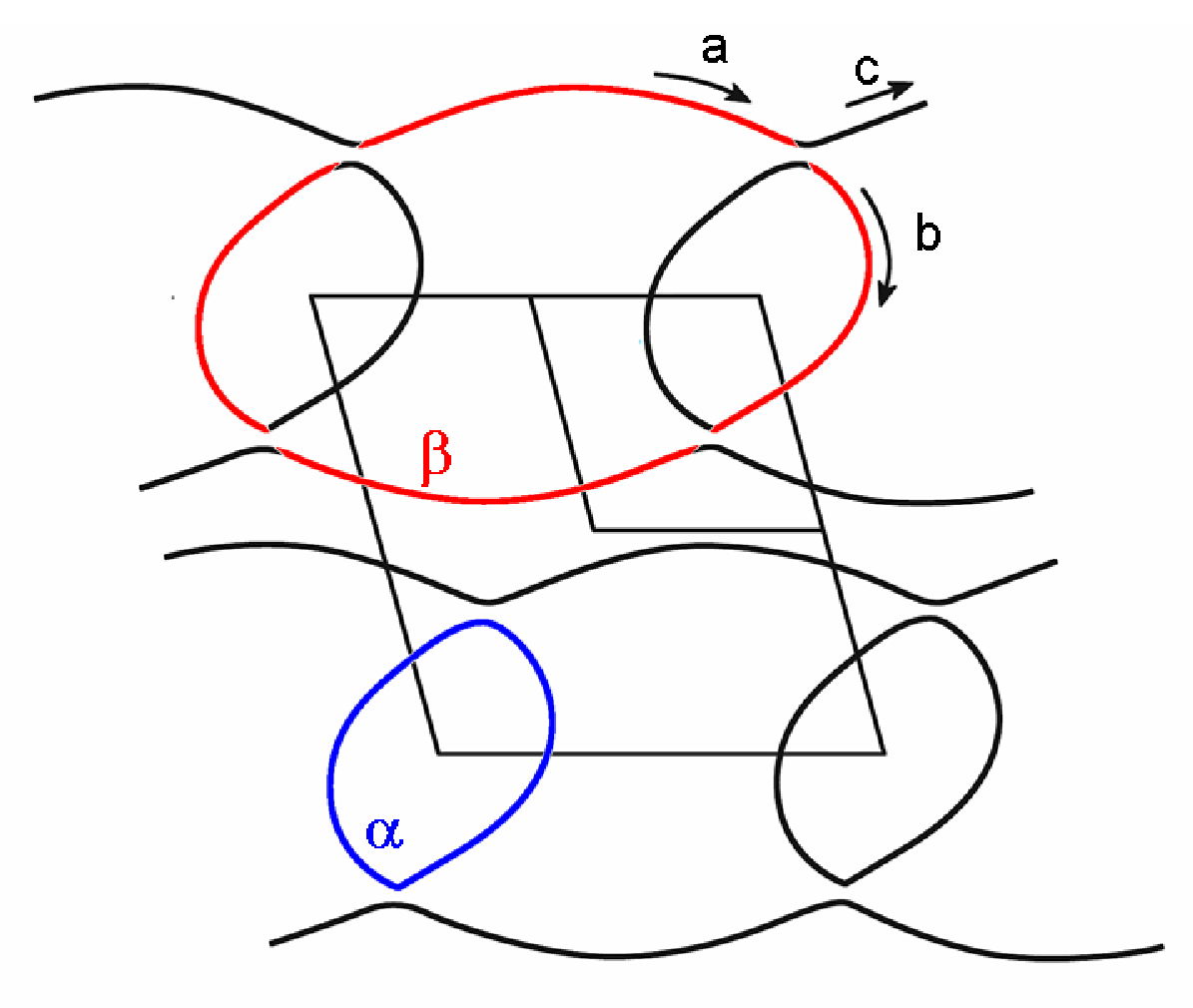
The main objective of this article is to consider the tunneling phenomena in interacting cyclotronic orbits, and its implication to the wavefunction characteristics at high and low field limits. In the first step of this paper, we review the problem of transmission and reflection coefficients within the S-matrix theory, when a particle coming from infinity is scattered by a tunneling region. From the simple model due to Rosen-Zener [12] and applied later to the magnetic breakdown case [5, 13], we focus on the effect of phase divergence in the S-matrix amplitudes. This actually occurs in different fields of physics, for example the level-crossing problem [14]. Amplitude ratio of the wave function is then considered in the second step when multiple paths are involved in the tunneling process, leading to an oscillatory behavior of the transmission coefficient. High field and semi-classical results are presented and compared to the numerical resolution of the Schrödinger equation. In the third step, we consider an exact approach to compute the quantum states in the interacting case of two circular orbits with bound state conditions. This new method is based on an extension of the usual (creation and annihilation) bosonic operators of the harmonic oscillator that includes effective coupling between the individual Fermi surfaces using two parameters, representing the coupling itself and the gap separately. This is an approach that can be easily generalized to a linear chain of coupled orbits, and which should give new insights on the wavefunction properties. Finally, consequences on experimental de Haas-van Alphen oscillations phase offset are considered for real FS of organic conductors.
2 Review of the transmission phenomena in a simple two-band model
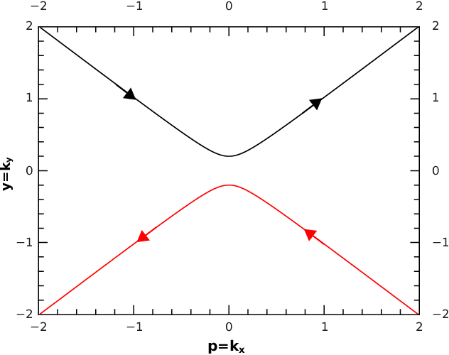
The presented model is intended to review the local transmission phenomena in two-band metals with MB junctions, the FS of which achieves a linear chain of coupled orbits (see e.g. [9, 15, 16]). A typical example of such Fermi surface is presented in Fig. 1 for (BEDO-TTF)5[CsHg(SCN)4]2 [11] (BEDO-TTF stands for the bis-ethylenedioxi-tetrathiafulvalene molecule), where an incoming amplitude (a) is transmitted to (b) and reflected to (c). At the vicinity of the MB junction, two linear sheets hybridized with energy constant can be considered. The local Fermi surface is represented on Fig. 2 for a non-zero coupling, and the linearized effective Hamiltonian can be written as
| (1) |
For , the two sheets and the wavefunctions and are independent. In such case, the MB gap which is proportional to , is zero. In presence of a magnetic field, the quantum representation of this model is chosen such that and , with . In this case, the differential equations for the wavefunctions are
| (2) |
where is an effective magnetic Planck constant 11 1 is not to be confounded with the real Planck constant that we will write in the rest of the paper. This set of first-order differential equations can be reduced using the transformation and , where now
| (3) |
where is a unitary matrix. We can notice that the product is diagonal, which makes easier the computation of any multiple products of
| (4) |
The solution of Eq. (3) is given by a series of matrix ordered products and multiple integrals [17]
| (5) |
Using the property Eq. (4) and setting ( can be a more general function of as we shall see later), one can write a transfer or S-matrix between two points and on the axis, away from the tunneling region
| (6) |
with by conservation of probabilities. The matrix elements are infinite sums of ordered integrals given by
| (7) | |||
where the are dummy variables. The characteristics of this matrix have been studied by many authors [18, 19] in the case of the Zener effect [12]. In the Gaussian case, when is quadratic, it is convenient to use the theta function representation in the complex plane [18] when . Indeed the diagonal matrix element can then be computed with the aid of simple translation transformations. For example, the double integral in the first line of Eq. (7) can be simplified by introducing , where the path in located on the upper half complex plane, to satisfy the constraint
| (8) |
The last integral is obtained after translating and respectively, to remove the couplings with . Then . All the terms in the series can be computed similarly, and the resummation leads to . We will introduce in the following the breakdown field which is characteristic of the tunneling process. The same techniques could be applied for elements , but one finds that the result is diverging in the large limit. The reason is that the phase of is diverging logarithmically [14], as we will see below, although the modulus is finite. A correct asymptotic analysis for finite and is therefore needed.
2.1 Asymptotic analysis
One can solve the equation for and using standard techniques. Indeed, the differential equation satisfied by can be obtained, separating from in Eq. (3)
| (9) |
The two odd and even solutions for are a combination of two Kummer fonctions [20] with an imaginary variable, and which can be chosen such that
| (10) |
where and are constant. Then and . We notice that there are only two constants in the problem, since from Eq. (9) is entirely determined by . The S-matrix Eq. (6) between points and can then be obtained by eliminating the coefficients and in Eq. (10). Setting
one can express the outgoing wavefunction and as function of an incoming wavefunction and as represented locally in Fig. 1
| (11) |
The functions depending on are given by Kummer functions
| (12) |
and the expression for the S-matrix elements is given by
Asymptotically, for large, one can use the expansion [21] and keep the dominant terms
| (13) |
and
| (14) |
Using the different duplication formulas for gamma’s functions: , , and , one obtains the probability of tunneling , which is the typical tunneling amplitude already obtained in many previous works [5, 13]. The breakdown field is in this case equal to and corresponds exactly to the semi-classical expression (see text further below). The remaining elements of the tunneling matrix can be obtained after some algebra and one finds the unitary matrix
| (15) |
where and the phase depends on the coordinate
| (16) |
The phase diverges logarithmically with . Since the FS is not accounted for by Fig. 2 for where it should be more curved, we assume that the phase is finite far from the tunneling region. Using a Stirling expansion of the gamma function in Eq. (16), one finds that is finite asymptotically only when . This corresponds approximately to the coordinate where the tunneling region ends, e.g. . In this case, instead of Eq. (16), the phase is given by the following regularization [5, 22]
| (17) |
The phase is zero in the low field limit ( large) and equal to when is large ( small).
3 Transmission through the small pocket
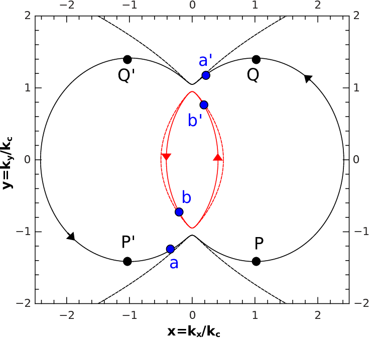
A more general model is given by an hybridization of two parabolic bands, whose Fermi surface is composed of two circular sheets, each of radius and centers , as displayed in Fig. 3, and for which the Hamiltonian reads
| (18) |
Rescaling the variables with and setting , , , and , one obtains
| (19) |
For small , one has the approximation near the tunneling points (points , , , and in Fig. 3)
| (20) |
This Hamiltonian gives a first order differential matrix equation, similar to Eq. (3), after setting and
| (21) |
with instead of . The first double integral in Eq. (7) contributing to in the large field limit and far from the scattering region can be written as
| (22) |
We can define each integral over and as a function of
| (23) |
Then using , one obtains
| (24) |
This expression is valid at large fields. It contains an imaginary part which is due to the presence of the small -orbit between points and , with area , in red in Fig. 3. Indeed, after tunneling through , the particle can be scattered multiple times around the orbit, and therefore acquires a phase proportional to , before exiting trough .
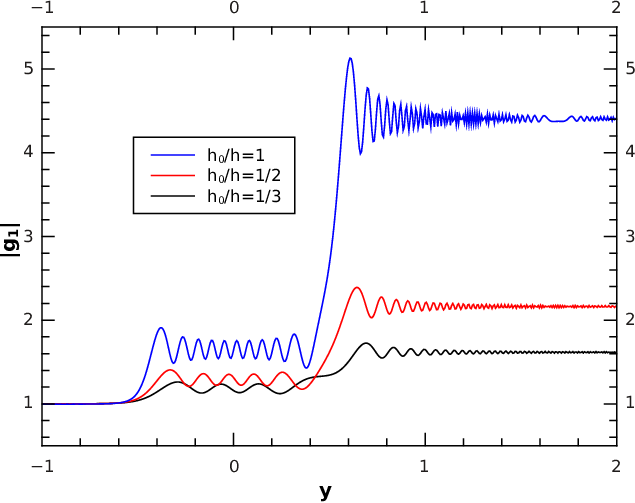
In the following we compare the transmission coefficient through the small -orbit to the expression given by the semi-classical relation and numerical results.
3.1 Semiclassical approximation
The Hamiltonian Eq. (20) leads to the set of differential equations for and
| (25) |
with 22 2 The solutions of Eq. (25) are actually given by triconfluent Heun functions [23]. In Fig. 4, we have represented the numerical solution of Eq. (21) and Eq. (25), in particular the modulus of for different values of fields. At large values of , we can approximate Eq. (25) by the equations and , which leads to constant, and constant. We have chosen and integrated numerically the first differential equation. On the far right, , the constant value is proportional to . Therefore, by computing , we can access to the breakdown field . The semi-classical approximation , where corresponds physically to an area enclosed by the trajectory, consists in expanding as a series in . In particular, at the leading order in for small field values, one can write with
| (26) |
When , as for the model Eq. (1) (linear sheets of Fig. 2), . The breakdown field is then given by the tunneling amplitude through the forbidden region, or , which corresponds to the exact result in this particular case. For the second model, Eq. (20) (parabolic sheets of Fig. 3), the breakdown field through one of the two tunneling regions, is instead given by
| (27) |
The phase variation of around the small pocket corresponds to the area of the pocket
| (28) |
where and are complete elliptic functions of the second and first kind respectively, and the approximation is taken when is small. For a unit cell parameter Å, or, equivalently, a unit cell area of 100Å2, which holds for the organic metals -(ET)4CoBr4(C6H4Cl2) and -(ET)2Cu(SCN)2, the frequency and magnetic breakdown field , expressed in Tesla are given by
| (29) |
As examples, the frequency of the two above salts is 944 T and 600 T, respectively, yielding = 0.55 and 0.48. The MB field is 35 T and 16 T, yielding = 0.015 and 0.01, respectively.
3.2 Transmission coefficient
We consider the probability of tunneling between points and in Fig. 3, using the model Eq. (20), which is defined by the modulus . Given the approximate value of in Eq. (24), we can estimate in the large field limit by exponentiating Eq. (24)
| (30) |
reaches its maximum, or resonance value , whenever the Airy function vanishes. This happens when , where are the zeroes of the Airy functions. For example , . A comparison with the numerical resolution of the differential equations Eq. (21) is shown in Fig. 5. The approximation presents a phase shift more pronounced as the field decreases.

Semi-classically, we can compute using the tunneling matrix Eq. (15) between the two points and in Fig. 3. It is the contribution of all possible trajectories between the two points, including the multiple reflections inside the -orbit
| (31) |
The factor corresponds to passing each of the two singular (or turning) points on the surface Fig. 3 where the slopes are infinite. The phase is taken from Eq. (17). Therefore one obtains (see [24])
| (32) |
is maximum when the field satisfies , e.g. , and the quantized values are given by
| (33) |
If , then .
(a)
 (b)
(b)

In Fig. 6 is plotted the transmission coefficient as function of the inverse field . The black continuous lines are obtained by solving the system of differential equations Eq. (21), with the condition , , , then by computing the ratio . Without the phase from the reflection coefficient Eq. (17), the values differ increasingly as the field is increased (dotted blue lines). Oppositely, the phase does not contribute to the oscillations when the field becomes small.
4 Amplitude ratios between two-interacting orbits
In this section, we consider the model Eq. (19), which represents the hybridization of the two giant orbits corresponding to the -orbit of the organic metals considered in the last section (see Fig. 1). Using the field quantization, one obtains the set of differential equations
| (34) |
As in preceding sections, we introduce two functions and such that . are two phase functions that are chosen such that the coefficient of vanishes in Eq. (34) after replacement. One obtains
| (35) |
The phase functions satisfy the differential equations
| (36) |
We can chose in particular and . The solutions of the Ricatti equations with respect to defined by Eq. (36) can be found in principle using hypergeometric functions. The coefficients and in front of the s in Eq. (35) can be removed using an additional transformation , such that
| (37) |
Then finally
The whole system can be cast into a system of first-order differential equations
| (38) |
with and defined by
| (39) |
The S-matrix can then be formally defined by ordered-integral iterations of the matrix functions and , similarly as Eq. (4). If we introduce and , one finds that the matrix element can be expanded as
| (40) |
which is equivalent to Eq. (7) found for one tunneling junction.
4.1 Case with no hybridization ()
In absence of hybridization, it is interesting to study the phase for an unbounded state (a state where one of the boundary condition for the wavefunction does not vanish at infinity). The two sheets decouple in this case, and one has only two independent linear second-order differential equations for and . Setting and , Eq. (34) becomes
| (41) |
where is the radius of the orbit. It is well-known that the even and odd solutions are expressed using two Kummer functions with as main argument [20]
| (42) |
Solution for the other function is similar with independent constants. We impose the constraint that, for large and negative, vanishes. This leads to the relation
| (43) |
In Fig. 7(a) is represented , with a vanishing boundary condition on the left. Only one constant remains, which is not relevant when we consider the ratio of the wave function between and in Fig. 3. Indeed the transmission factor defined here by is exactly equal to
| (44) |
and is a function of . In physical units, the ratio is equal to the -orbit frequency (in Tesla) divided by the magnetic field
| (45) |
which is usually a large number ( is few thousands of Tesla for organic conductors). It has to be noticed that imposing a vanishing wavefunction at both negative and positive large values of (bound state) leads to two conditions
| (46) |
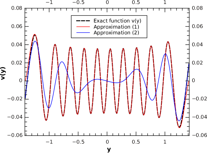
which can only be satisfied when the gamma functions are infinite. This happens when both arguments of the gamma functions are negative integers, and one obtains the usual quantification relation or Landau levels with positive integer. Using the different asymptotic expansions for the Kummer function [21], one obtains for each wave function and a good approximation near the turning points (see Fig. 7(b), and (c), approximation (2))
| (47) | |||
| (48) |
In the region , not too close to the turning points, the solutions are instead adequately approximated by (see Fig. 7(b) and (c), approximation (1))
| (49) | |||
| (50) |

(a)
 (b)
(b)
 (c)
(c)
Moreover, the ratio between the two constants and in Eq. (43) is approximated by
| (51) |
Using Eq. (47) and Eq. (48) for , and , one obtains the semi-classical limit of the inverse transmission factor, and after some algebra and simplifications one obtains the simple result
| (52) |
The frequency of the oscillations is as expected, but there is a shift equal to as opposed to the semi-classical limit, which is equal to for a bound state or localized wavefunction, where at each turning point a Maslov factor equal to is involved after total reflection of the wave function.
4.2 Semi-classical analysis for interacting orbits
In this section, one computes semi-classically for a bound state the amplitude ratio between points and in Fig. 3, using a transfer matrix method to obtain all the contributions from the different electronic paths. One has indeed to evaluate the sum of all the amplitudes corresponding to multiple orbits connecting the two points and , with their harmonics, and using the connection formula Eq. (15) for the tunneling regions. In Fig. 3, we have represented 4 different points (amplitudes) . and belong to orbits or , and and belong to orbits or . These points are located just before the tunneling event, such that there is a possibility to be transmitted or reflected, just after passing trough the breakdown points. A trajectory is an ensemble of steps on the surface, which connect to . At time we start from . At later time , we can write the amplitudes as function of the amplitudes at time . For example amplitude at time is the sum of after reflection and after tunneling at time , and can be written as . There are 3 other equations connecting the different points at each step on a trajectory. At , , and we introduce a phase shift . One can write therefore the system
| (53) |
From these relations, we can define a step matrix , acting on vector , with initial condition . Then , with
| (54) |
where and . We define which is also equal to
| (55) |
Only the even powers of contribute since to go trough twice we need to perform an even number of steps. Resumming the expression in Eq. (55) involves the inverse of which can be computed from since is simply the diagonal block matrix , and therefore . After some algebra, we extract the third component of to obtain
| (56) |
There are two obvious cases. When and , one obtains , or , which was obtained previously in Eq. (52). Oppositely, when and , the particle describes orbits around , and , or . This expression depends on explicitly.
4.3 Simple solvable model for two-interacting orbits
Let us rewrite the Hamiltonian Eq. (19) in the representation . One obtains the set of coupled differential equations
| (57) |
The advantage of this representation is that the imaginary parts in Eq. (34) are absent, at the cost of a shift in the harmonic potential. Function is centered around whereas function has dominant weight around . We will consider instead a slightly different set of equations
| (58) |
where is a parameter and the coupling is a function of : with constant. The Hamiltonian operator is then defined by
| (59) |
and the Fermi surface is the location of points given by the equation
| (60) |
For and non zero, the surface is composed of two sheets separated by a gap proportional to , see Fig. 8(a). It has to be noticed that for this particular choice of coupling function, there is no observable gap on the Fermi surface when , since , but the two surfaces are still coupled at other points by , see Fig. 8(b). The advantage of the Hamiltonian Eq. (59) is that it can be factorized using simple bosonic operators associated with centers in the complex plane :
| (61) |
with . The set of differential equations Eq. (58) are indeed identical to two coupled harmonic oscillators
| (62) |
and it is straightforward then to consider the following two-dimensional ’bosonic’ operators
| (63) |
to express the Hamiltonian as an extended harmonic oscillator in two-dimensions
| (64) |

(a)
 (b)
(b)
The ’bosonic’ operators and satisfy the commutation relation
| (65) |
which is not unity when the product is not zero. We cannot therefore call them ’bosonic’ in the usual sense since there is a mixing of the two different types of bosons due to the coupling. Here are the usual Dirac matrices in two dimensions 33 3 We remind that the Dirac matrices are defined by , , , and . There are two possible ways to construct the wavefunctions, depending on the value of . If , then and are true bosonic operators, and we can construct the ground-state solution of lowest energy , with . This imposes the constraint on the field. Normally we construct the states above the ground state energy by quantization of the area, or , but here we keep constant (or constant Fermi energy) and solve for values for which a set of bounded wavefunctions can be found. It is easy to see that the first component satisfies the factorized differential equation
| (66) |
The solutions are simple combinations of two Gaussian exponentials centered at
| (67) | |||


The two components are coupled together once the constants and are determined. These constants satisfy a conservation equation, depending on the filling factor. If we consider initially a system filled with one electron in each orbital at zero coupling, therefore two electrons in total, we impose that, by increasing the coupling, the number of electrons per orbital does not change. One has the pair of constraints (in this case we consider real functions), which leads to , and to the following relations of conservation
| (68) |
The other state vectors at higher energy (or higher nodes) are given by the successive application of on
| (69) |
with energy . When , this imposes a field value for which is solution of Eq. (57). In figure Fig. 9, we have represented the two components and for the state at constant . In the limit of small coupling, Eq. (68) leads to the solutions (we choose and )
| (70) | |||
which is expected for two independent orbitals. In general, the two constants and are not independent because of Eq. (68), which leads to an effective coupling between the two components of the wavefunction.
Let us now consider the case . The ground state is still defined by . Setting , one obtains
| (71) | |||
The conditions of normalization are the same as before, which leads to a set of complex equations similar to Eq. (68). The commutator Eq. (65) prevents us to construct the excited states , which satisfies , directly from successive applications of on the ground state. Instead we have to seek for linear combinations of functions
| (72) |
where are constant matrices to be determined self-consistently. In the limit , only the matrix does not vanish, and corresponds to the normalization factor. Computing leads to a set of relations between these matrices at order . In particular, by application of on each element of Eq. (72), one has
| (73) |
For the last two terms, after some algebra, we can move the operator to the right of and using the binomial relation
The matrices are zero when , and in this case we have simply . The identification of each coefficient of in the equation leads to the set of equations which are composed of commutators. In particular, the first three equations read
| (74) | |||
This can be solved for example using Dirac matrices with unknown scalar coefficients. For example, the matrix coefficients of the first excited state , , can be found by solving the two equations
| (75) |
It is useful to write and using Dirac matrices
and separate the part proportional to identity from the remaining ’s: and , with constant matrices
and . Differential operators and are proportional to the identity matrix and commute with and which are constant matrices. Then the solutions of Eq. (75) can be expressed using and only. An obvious solution of the first equation is , where and are constants which are determined by orthogonality and normalization of the wavefunctions and . Then a solution of the second equation is simply . In particular, this leads to the factorization
| (81) |
Writing the condition leads to
| (82) |
The normalization gives a supplementary condition which fixes the two constants (up to a phase factor)
| (83) | |||
where we have omitted in the scalar products to simplify the notations. When no coupling is present , , and . We also assume that in this case that , so that and , which corresponds to the uncoupled model of two electrons in two independent orbits. This method allows for the construction of all excited states and can be generalized for a linear chain of coupled orbits. Indeed we can represent the and operators as extended matrix operators of dimension with coupling parameters and similar to Eq. (63), and centers corresponding to each individual oscillator. For example, in Fig. 10, we have represented such surface, for connected orbits, by considering the following extended bosonic operators in four dimensions

| (84) |
and
| (85) |
5 Onsager phase of de Haas-van Alphen oscillations in linear chains of coupled orbits

In this section, we consider de Haas-van Alphen oscillations observed in quasi-two-dimensional organic metals with a Fermi surface which can be regarded as a linear chain of orbits coupled by magnetic breakdown. Recall that Fourier spectra of these compounds is composed of Fourier components, labeled in the following, the frequency of which are linear combinations of that linked to the closed orbit and the magnetic breakdown orbit : = . The field- and temperature-dependent amplitude of several of these components does not follow the usual Lifshitz-Kosevich formula due to oscillation of the chemical potential in magnetic field. Nevertheless, Fourier amplitudes are accounted for by a development up to the second order in damping factors in this case [15, 16, 10]. An extensive discussion of this problematic is given in Refs. [25, 26]. As an example, let us consider magnetic torque data relevant to the organic metal -(ET)4CoBr4(C6H4Cl2). Field- and temperature-dependent de Haas-van Alphen oscillations amplitudes of this organic metal are consistently accounted for by this formalism with the following parameters: = 944 4 T, = 4600 10 T, = 1.81 0.05, = 3.52 0.19, = = 1.9 0.2, = = 0.79 0.10 K, = 35 5 T, where , , , and are the frequencies, effective masses, effective Landé factors, Dingle temperatures and magnetic breakdown field, respectively [15]. Furthermore, the Onsager phase of the various Fourier components is accounted for by Eq. 17, yielding [10]
| (86) |
where is the number of reflections events and is equal to times the number of turning points of the orbit. De Haas-van Alphen oscillations of Fig. 11 are obtained with this set of parameters, except that various values of are explored. As expected, as , hence the reflection probability , increases, the amplitude of all the components involving decreases and, at very high , only remain the contributions of and its harmonics. The striking point, on which we will focus in the following, is the observed shift of the oscillations, for which [25, 26], as varies (whereas the Onsager phase of oscillation remains unchanged since = 0 [10]).
Strictly speaking, the oscillations are not periodic in for finite values. This effect can be quantified considering an ’apparent frequency’ = where the indexes and mark two successive oscillation maxima. According to Eq. 86, = + , yielding an ’universal’ frequency shift:
| (87) |
where = , which depends on , e.g. on the ratio , only, for a given value.

Data of Fig. 12 displays the frequency variations of the component. Reported experimental data deal with magnetic fields of up to 56 T [10], e.g. with maximum values of 1.6. According to the data of Fig. 12, the corresponding frequency shift is F = 3 T which is within the reported error bars (since = 944 4 T for the considered compound). Nevertheless, frequency shift predicted by Eqs. 17, 87 could be detected in the future at higher magnetic fields and for orbits involving larger number of reflection events such as observed in two-dimensional networks (see [27]).
6 Summary and Conclusion
Calculation of transmission and reflection coefficients through a magnetic breakdown junction have been reviewed with the aim of determining the Onsager phase of de Haas-van Alphen oscillations. The problem of the phase divergence of the S-matrix describing wave function transmission has been addressed by suitable asymptotic analysis. Amplitude of the wave function was then calculated, using approximate and exact models of connected Fermi surfaces, yielding the field-dependent phase offset relevant to de Haas-van Alphen oscillations for Fermi surfaces with magnetic breakdown. As a consequence, experimental de Haas-van Alphen oscillations are not strictly periodic in for orbits with reflections at the magnetic breakdown junctions. Nevertheless, frequency variations, which follow a ’universal’ field dependence remain small within realistic experimental conditions.
References
References
- [1] Mikitik G P and Sharlai Y V 1999 Phys. Rev. Lett. 82(10) 2147–2150
- [2] Fuchs N J, Piéchon F, Goerbig O M and Montambaux G 2010 The European Physical Journal B 77 351–362
- [3] Wright A R and McKenzie R H 2013 Phys. Rev. B 87(8) 085411
- [4] Fortin J Y and Audouard A 2015 The European Physical Journal B 88 1–7
- [5] Slutskin A and Kadigrobov A 1967 Sov. Phys. Solid State 9
- [6] Slutskin A 1968 Sov. Phys. JETP 26 474–482
- [7] Huang W and Taylor P L 1976 Phys. Rev. Lett. 36(4) 231–233
- [8] Pippard A 1962 Proc. R. Soc. London A 270 1
- [9] Oshima K, Mori T, Inokuchi H, Urayama H, Yamochi H and Saito G 1988 Phys. Rev. B 38(1) 938–941
- [10] Audouard A, Fortin J Y, Vignolles D, Lyubovskii R B, Zhilyaeva E I, Lyubovskaya R N and Canadell E 2013 Synthetic Metals 171 51 – 55
- [11] Lyubovskiĭ R, Pesotskiĭ S, Biberacher W, Zhilyaeva E, Bogdanova A and Lyubovskaya R 2008 Physics of the Solid State 50 1560–1564
- [12] Rosen N and Zener C 1932 Phys. Rev. 40 502–507
- [13] Chambers W 1968 Phys. Rev. 165 799–809
- [14] Torosov B T and Vitanov N V 2011 Phys. Rev. A 84(6) 063411
- [15] Audouard A, Fortin J Y, Vignolles D, Lyubovskii R B, Drigo L, Duc F, Shilov G V, Ballon G, Zhilyaeva E I, Lyubovskaya R N and Canadell E 2012 EPL (Europhysics Letters) 97 57003–
- [16] Audouard A, Fortin J Y, Vignolles D, Lyubovskii R B, Drigo L, Shilov G V, Duc F, Zhilyaeva E I, Lyubovskaya R N and Canadell E 2015 Journal of Physics: Condensed Matter 27 315601
- [17] Lam C 1998 J.Math.Phys. 39 5543–5558 (Preprint hep-th/9804181)
- [18] Rojo A G Matrix exponential solution of the landau-zener problem equation (20) (Preprint http://arxiv.org/abs/1004.2914v1)
- [19] Kholodenko A and Silagadze Z 2012 Physics of Particles and Nuclei 43 882–888
- [20] Holmes M H 1995 Introduction to perturbation methods Texts in applied mathematics (New-York: Springer-Verlag) page 299
- [21] Abramowitz M and Stegun I 1984 Pocketbook of mathematical functions (Thun, Frankfurt am Main: Verlag Harri Deutsch) asymptotic forms for large argument in the Kummer function are given in 13.5.1. For small , the two asymptotic expansions for and are given respectively by 13.5.19 and 13.5.21 with
- [22] Kochkin A 1968 Sov. Phys. JETP 27 324–327
- [23] Hortaçsu M 2012 Heun functions and their uses in physics (World Scientific Publishing Company) chap 2, pp 23–39 (Preprint arXiv:1101.0471)
- [24] Kaganov M and Slutskin A 1983 Phys. Rep. 98 189–271 (See eq. 5.22 and figures 17 and 19a)
- [25] Audouard A and Fortin J Y 2013 Comptes Rendus Physique 14 15 – 26
- [26] Audouard A and Fortin J Y 2014 Low Temperature Physics 40 344–351
- [27] Laukhin V N, Audouard A, Fortin J Y, Vignolles D, Prokhorova T G, Yagubskii E B and Canadell E 2017 Fiz. Nizk. Temp. this issue