0 \vgtccategoryResearch \vgtcinsertpkg\authorfooterJean-Daniel Fekete is with INRIA. E-mail: Jean-Daniel.Fekete@inria.fr Romain Primet is with INRIA. E-mail: Romain.Primet@inria.fr \shortauthortitleFekete & Primet: Progressive Analytics \CCScatlist\CCScatK.6.1Management of Computing and Information SystemsProject and People ManagementLife Cycle; \CCScatK.7.mThe Computing ProfessionMiscellaneousEthics
Progressive Analytics:
A Computation Paradigm for Exploratory Data Analysis
Abstract
Exploring data requires a fast feedback loop from the analyst to the system, with a latency below about 10 seconds because of human cognitive limitations. When data becomes large or analysis becomes complex, sequential computations can no longer be completed in a few seconds and data exploration is severely hampered. This article describes a novel computation paradigm called Progressive Computation for Data Analysis or more concisely Progressive Analytics, that brings at the programming language level a low-latency guarantee by performing computations in a progressive fashion. Moving this progressive computation at the language level relieves the programmer of exploratory data analysis systems from implementing the whole analytics pipeline in a progressive way from scratch, streamlining the implementation of scalable exploratory data analysis systems. This article describes the new paradigm through a prototype implementation called ProgressiVis, and explains the requirements it implies through examples.
keywords
Analytics, Visualization, Big-Data, Scalability, Interaction1 Introduction
Data analysis systems delivering their results in a progressive manner have become more popular in the recent years [7, 8, 12, 13, 15, 33, 41, 43], but their implementation has, so far, been ad-hoc. This article describes a novel computation paradigm we call Progressive Analytics, aimed at improving the scalability of exploratory data analysis systems. To concretely explain implementation issues, we also describe a proof-of-concept implementation of our paradigm: a Python toolkit called ProgressiVis. Progressive Analytics, and therefore ProgressiVis, is designed to support the implementation of exploratory analysis systems that compute and return results in a progressive way at the language and library level. Moreover, Progressive Analytics provides mechanisms to support user interactions while the system runs, allowing filtering data, changing parameters, and even steering algorithms: all the underlying mechanisms needed to support visualization and visual analytics.
Existing analytics system rely on sequential computations to deliver their results, i.e. if a function operates on results of a function , it has to wait for to finish before starting to run. The main issue addressed by the Progressive Analytics computation paradigm relates to one intrinsic limitation of sequential systems: their latency. With current systems, computation time can grow without bounds when exploring large datasets or when using complex analysis methods on the datasets. However, when performing exploratory analysis, humans need a latency below about 10 seconds to remain focused and use their short-term memory efficiently [24, 40]. Sequential systems cannot guarantee such a latency so there is always a large-enough dataset or complex-enough computation that leads sequential systems to exceed this limit and become unusable for exploration. Distributing and parallelizing computation increases the overall speed, but does not change the sequential paradigm: the time to obtain the results of a computation has no guaranteed bounds unless the programmer implements these bounds in the software somehow.
In contrast, the Progressive Analytics computation paradigm is designed to always produce partial results of computations under user-specified bounds, allowing the system to comply with the human cognitive constraints. A major divergence from sequential systems is that Progressive Analytics systems do not deliver the whole computation at once; instead, they generate a sequence of partial results that converge to the final results. Meanwhile, users can interact with Progressive Analytics systems to change parameters of the computation, instead of waiting to completion to change them. Analysts can also make decisions before the end of the computation if they feel confident about it. These early decisions are very important in exploratory settings [33].
Due to their appealing properties, over the last decade, many experimental systems delivering progressive results have been implemented, demonstrated, and described in scientific publications, over the whole range of topics related to analytics: databases [15], computations and machine-learning [33, 43], visualization [7, 25, 41, 43], and user interfaces [8, 12, 13]. However, all these systems rely on ad-hoc software architectures, none of them claiming to be designed in a modular fashion or reusable. Today, creating a new progressive system implies reimplementing almost completely all the components from data management to user interfaces; an overly expensive endeavor. To address this software architecture problem so as to streamline the development of good-quality progressive systems, we have designed the ProgressiVis toolkit as an experimental platform to build progressive steerable exploratory systems in Python.
The contributions developed in this article are:
- •
a formal description of the Progressive Analytics computation paradigm to clarify the main properties needed for a system to claim “progressiveness”,
- •
a description of the ProgressiVis experimental implementation of the paradigm to show its practicality and the challenges ahead.
The article is organized as follows: the background section details the cognitive reasons why progressive systems are needed for exploratory analytics, defines formally what we call the ‘‘Progressive Computation’’ paradigm, and how previous work has addressed the issues raised by the Progressive Analytics computation paradigm. We then provide a detailed description of the ProgressiVis toolkit, through the implementation of example applications and a discussion11 1 This article supersedes the workshop note [11]..
2 Background
Computer users are already familiar with progressive behaviors: the progressive loading of web pages, where text appears initially with a rough layout, followed by images also progressively loaded, until the web page layout tidies-up to adopt its final appearance. Specific mechanisms have been built in web browsers, image file formats, and the HTML document format to support this progressive behavior and prevent users from waiting idly while the web page and its components get downloaded. Progressive Analytics can be seen as an extension of these behaviors for exploratory analytics where the guaranteed progression of computation and the ability to interact at any time to steer the analysis are an integral part of the analyst’s activity.
2.1 Latency, Cognitive Constraints and Exploration
When exploring data, analysts operate in a tight loop where they plan
for one analysis—expecting to obtain new information about the data,
launch the appropriate algorithm, and wait for the result to confirm
or infirm the expectation. The result arrives with some
latency.
Multiple studies have shown that humans have
perceptual and cognitive limitations related to that latency.
Miller’s seminal article on the effect of computer response time
distinguishes several orders of magnitudes for latency
summarized by Nielsen in [29, Chapter
5] and [30] (the latency names are
added by us):
Continuity Preserving Latency is about the
limit for having the user feel that the system is reacting
instantaneously, meaning that no special feedback is necessary
except to display the result.
Flow Preserving Latency is about the limit
for the user’s flow of thought to stay uninterrupted, even though
the user will notice the delay. Normally, no special feedback is
necessary during delays of more than but less than
, but the user does lose the feeling of operating
directly on the data.
Attention Preserving Latency is about the
limit for keeping the user’s attention focused on the dialogue. For
longer delays, users will want to perform other tasks while waiting
for the computer to finish, so they should be given feedback
indicating when the computer expects to be done. Feedback during the
delay is especially important if the response time is likely to be
highly variable, since users will then not know what to expect.
Exploratory data analysis is concerned primarily with analytical tasks where preserving attention and flow are always essential. For visual analytics where graphical interaction is required, continuity preserving latency is essential during direct manipulation [39] phases.
Liu and Heer [20] have studied the effect of continuity preserving latency during direct manipulation. They showed that “initial exposure to delays can negatively impact overall performance even when the delay is removed in a later session”. Therefore, a latency under 0.1 second is essential during direct manipulation and should be supported by an analytics system using visualization.
Regarding the user’s attention, Miller also argues that “The graphical response should begin within 2 seconds and certainly be completed within 10 seconds if the user is to maintain thought continuity in an ongoing task.” [24]. Shneiderman provides similar bounds: “These long delays may or may not increase error rates in the range 3–15 seconds, but they will probably increase error rates above 15 seconds […]. Dissatisfaction grows with longer response times.” [40].
Waiting for task completion while keeping user’s attention can be improved using techniques called Time Engineering or Time Design [38]. In particular, several techniques have been used to improve the progress bar to lower the frustration caused by waiting, and provide a better estimate of the waiting time [14, 28]. Even if some techniques only allow increasing the response time without raising too much frustration, others such as modern progress bars provide some information while waiting for an operation to complete. Indeed, the goal of [38] is to “Build Applications, Websites, and Software Solutions that Feel Faster, More Efficient, and More Considerate of Users’ Time!”. In that sense, Progressive Analytics is certainly a Time Engineering technique. To achieve this goal, few strategies are possible:
- 1.
Increasing the computing speed, but that approach has well-known physical limits due to the speed of light both for computing and for transmitting data;
- 2.
Pre-computing indexes or aggregates to speed-up the most common analytical queries. However, it is almost impossible to pre-compute enough indexes/aggregates to guarantee an acceptable latency during open-ended explorations. Furthermore, this pre-computation can be very long [19], and delays the moment when data can be explored;
- 3.
Leaving the exploration to some machine intelligence that does not suffer from the human cognitive constraints. However, intelligent systems are not yet able to replace human analysts, they are mainly used to provide hints and suggestions on interesting properties of data by computing e.g. correlations and searching remarkable properties in data;
- 4.
Use progressive analytics, as argued in this article.
Note that these strategies are by no means mutually exclusive; they can and should be combined eventually.
2.2 Definition
The word progressive has been used in many articles but, to our knowledge, never formally defined. Let be a function with parameters and yielding a result value . In mathematics, the value calculated by does not involve any time:
In computer science, a computation takes a time , uses an amount of memory , starts with a machine state , and modifies this state that becomes . Also, for analytics, we distinguish the parameters of the function from a set of input data tables that the function takes as input, and the ones it returns as output . Our mathematical function becomes a computation function :
| (1) |
For example, if is a function computing a clustering with the k-means algorithm (e.g. [22]), it will take as parameters (P) the number of clusters , a tolerance for the convergence of the algorithm, and possible many others depending on the actual implementation. It will also take one data table as input (D), and return two data tables as output (R): the cluster centroids, and a data table associating each input data item to its cluster.
The progressive computation of , noted , is a function with three properties:
- 1.
When called repeatedly on , a growing subset of , it returns a sequence of partial results , each result being computed with duration time (Equation 2);
- 2.
If is the desired amount of time between two consecutive partial results (the quantum), ;
- 3.
The results will converge to (Equation 3).
We will call an eager function, and a progressive function.
| (2) |
Formally, the growth of the data tables can be modeled with a partition of into non-intersecting subsets (chunks): . is therefore called with . Note that does now have to grow, i.e. some can be empty.
If analysts use directly for their computation, should be below according to the previous section. If is used as part of a sequence of operations seq, its quantum should be set so that the time to compute seq is below . This time constraint implies that progressive functions are real-time, but our cognitive quantum, even when split to deal with sequences, is much larger than the fractions of a second that computer-science traditionally expect for real-time constraints. Also, note that our definition does not set any constraint on the memory usage of . We will contrast this with other related concepts in the next section.
We also expect that our partial results will improve all along the computation so we define a convergence criteria for the progressive computation of :
| (3) |
If we define a distance to measure the amount of changes between two results, we would like our partial results to always improve, i.e. , but, in practice, we cannot guarantee it. Instead, for Equation 3 to hold, all we need is the Cauchy convergence criteria for a sequence, which states that, after some step , the results converge. We would like the convergence to happen as quickly as possible ( to be as small as possible) but this will depend on the function , the parameters , the data tables , the computation method that we use, and the distance function that we pick. For example, using simulated annealing, the early solutions are often made worse on purpose before they improve. Also, the convergence criteria in Equation 3 can be too strong and there may be some error between the exact direct computation of and its progressive computation. Note that the issue of errors in computation is not specific to our progressive functions.
From the definitions above, we can see that progressive functions can be composed just like eager ones because we know from calculus that, if is continuous at and , then:
| (4) |
Practically, in analytics, there are two main causes for long computations: 1) input/output time, and 2) computation time. If is a progressive function that loads a large dataset and computes some derived value from it, then Equation 4 insures that will converge to the final value progressively as the file is being loaded ( grows). Conversely, if computes a complex value derived from (e.g. a multidimensional scaling over a 1 million rows dataset already loaded so does not grow), then will also converge when the iteration converges. Though the mathematical foundations are sound, practical choices should be made carefully since they will affect how useful the progressive results will be. As stated by Stolper et al. [41]: “This method [progressive visual analytics] is based on the idea that analytic algorithms can be designed to produce semantically meaningful partial results during execution.”
2.3 Comparison with Related Concepts
Several concepts related to progressiveness exist in analytics, such as online, streaming, and iterative. Using the same formalism as in Section 2.2, we clarify their meaning and outline the similarities and differences to our progressive functions.
Online [5] is related to the way the data tables are made available to the function . Informally, an online function will provide partial results quickly when given data tables filled incrementally. Online algorithms are popular in machine learning and analytics in general, in particular to handle dynamic data. When is called iteratively with the growing subsets , it performs its computation efficiently:
Online algorithms guarantee that the total time to compute () is much shorter than the total time to compute each step independently (restarting the process with ). For most online algorithm, the total time is assumed to be independent of the partitioning . Just like progressive functions, online functions imply convergence (Equation 3). Contrary to progressive functions, online functions offer no guarantee that .
Online algorithms can be made progressive if there is a guarantee that feeding the data tables in small-enough chunks will not exceed a desired quantum. Then, an online function can be made progressive by making sure that it will be fed with data tables in small-enough chunks through a function that will split its inputs when necessary: . The challenge is then to find the best size of the chunks to match the time constraint. Feeding the data tables one row at a time as many times as necessary to fill-up the quantum is a possible strategy but usually implies a huge overhead compared to feeding larger chunks at a time. If the online algorithm cannot process its input under a quantum, it cannot be transformed into a progressive algorithm through the splitting function alone.
Streaming [27] is related to memory usage and time constraints. According to Wikipedia: “streaming algorithms are algorithms […] in which the input is presented as a sequence of items and can be examined in only a few passes (typically just one). These algorithms have limited memory available to them (much less than the input size) and also limited processing time per item.” Given these constraints, streaming algorithms can sometimes compute rough approximations of the theoretical results. Streaming algorithms are progressive by design and can be used in progressive systems, although the quality of the results they provide can be a practical problem. Also, streaming algorithms are usually difficult to design and implement; relying only on streaming algorithms to implement an analytic infrastructure would fit the theoretical needs but severely limit the range of possible applications that could be built. For example the Spark streaming machine-learning library [32] provides 86 classes compared to the 245 provided by the scikit-learn machine-learning library [31]. In comparison to progressive functions, streaming functions have limited memory, implying constraints on in Equation 2.
An Iterative (e.g. [35]) method is defined in Wikipedia as: “a mathematical procedure that generates a sequence of improving approximate solutions for a class of problems.” An iterative method performs its computation through some internal iteration and can usually provide meaningful partial results after each iteration, although some extra work might be required to obtain the partial result in an externally usable form. Iterative methods have a behavior similar to Equation 2, except they do not take chunks but the whole dataset at each iteration. They also comply with the convergence of Equation 3. However, being iterative does not imply any bounds in the execution time of each iteration. If the iterations are always shorter than a specified quantum, they can become progressive for that quantum.
The family of progressive algorithms is the only one explicitly aiming at user-oriented properties and guarantees. All the other methods are oriented towards fulfilling machine-oriented properties, not guaranteed to be suitable for data exploration.
2.4 Analytics and Machine-Learning
Analytics and Machine-Learning have been concerned with online and streaming methods for a long time, even if data exploration has rarely been the main rationale for these topics. Additionally, many methods related to exploratory data visualization at scale have been pursued.
Many well-known statistical measures can be computed online or on streams with little adaptation, including average (mean), variance, standard deviation, and many linear models. There are online and streaming variants for all the families of machine-learning algorithms, as described by Mühlbacher et al. [25]: classification, regression, clustering, dimensionality reduction, and preprocessing methods (e.g. mean removal and variance scaling). However, few libraries or toolkits provide a consistent software engineering abstraction to use the progressive algorithms, with the exception of the Spark Machine-Learning library [32] that provides several streaming implementations to use with the Spark cluster programming environment [44]. In most cases, the APIs to use these algorithms are ad-hoc and very diverse.
In addition to algorithms that are natively online or streaming, substantial work has been invested into adapting incremental algorithms to become progressive. Stolper et al. [41] report on how they adapted the SPAM algorithm [3] to meet the progressive requirements. Mühlbacher et al. [25] mentions 4 strategies to increase “user involvement”, their particular interpretation of progressiveness, and list 12 algorithms that can be made progressive with different levels of integration. Directly related to progressive analytics, Pezzotti et al. [33] present a full progressive pipeline for the t-SNE multidimensional technique. This line of articles shows that a large family of costly iterative projection methods can be adapted to become progressive and even steerable.
Algorithm steering is defined as “interactive control over a computational process during execution” by Mulder et al. [26]. Progressive methods are steerable if the user can control the computation while the system progressively processes the rest of the dataset. Controlling means either changing some control parameters, or specifying interactively that a selection of the data is more important to the user, and that the system should deliver faster and more accurate progressive results for that selection. Work described in [25, 33, 41, 43] support steering.
2.5 Visual Analytics
Visual Analytics has been interested by two issues related to progressive analytics: system infrastructures and HCI/cognitive issues.
On the system infrastructure side, the closest system to ours is PIVE [7], and, to a lesser degree, In-Situ visualization systems [21]. PIVE [7] allows monitoring the progress of iterative algorithms running and sometimes even steer them using a different approach than ours. It instruments the iterative algorithms to communicate with a visualization and interaction thread running in parallel to the main execution thread. The instrumentation is in charge of sending the right parameters to the visualization and interaction threads. Using this approach, users create their program as before; there is almost no impact on the implementation, except that instrumentation comes afterwards and need to prepare the data for sending to the visualization and interaction thread. Some instructions can also be sent in return from the visualization and user-interface to steer algorithms, so the logic needs to be inserted in the original algorithm. This approach is also very close to In-Situ visualization [21], a paradigm used mostly in high-performance computing where monitoring the progression of algorithms is very important but cannot involve too much data transfer or program interruption because the algorithms are implemented to use the parallel computing infrastructure in the best possible way, and the data is just too large and dynamic to be moved. In-situ visualization consists of instrumenting the simulation code to allow as much exploration as possible in the computed data without disturbing the computation too much. Using these monitoring approaches, the system remains algorithm driven and not data or analyst driven. While this is the goal of In-situ visualization or algorithm visualization where visual exploration is performed over the data generated by the algorithm/simulation, general data exploration may require more flexibility, such as trying several algorithms and parameters to select an effective combination, or other operations that do not consider the algorithm as being fixed upfront.
Stolper et al. [41] enumerate seven important design goals for progressive visual analytics applications. These goals are related to the exploration process when performed using a progressive system. “First, analytics components should be designed to:
- 1.
Provide increasingly meaningful partial results as the algorithm executes
- 2.
Allow users to focus the algorithm to subspaces of interest
- 3.
Allow users to ignore irrelevant subspaces
Visualizations should be designed to:
- 4.
Minimize distractions by not changing views excessively
- 5.
Provide cues to indicate where new results have been found by analytics
- 6.
Support an on-demand refresh when analysts are ready to explore the latest results
- 7.
Provide an interface for users to specify where analytics should focus, as well as the portions of the problem space that should be ignored”
We have discussed Goal #1 in the beginning of the Background section. The other goals are related to capabilities that progressive systems should offer, and more cognitive and HCI aspects of progressive systems. An infrastructure supporting the implementation of progressive systems should provide the mechanisms to reach the listed goals. Unfortunately, the article does not provide enough implementation details to compare it to our paradigm.
Finally, Mühlbacher et al. [25] describe strategies to convert algorithms to become progressive and steerable for a deeper user involvement. From a user’s perspective, the progressiveness is part of what they call the feedback properties, and steering is part of the control properties. The listed properties are essential for progressive systems and should be implemented in the lower layers of progressive systems, such as progress feedback, cancellation, prioritization, etc. They also describe 4 possible strategies to achieve their desirable properties: 1) Data subsetting, 2) Complexity selection, 3) Divide and combine, and 4) Dependent subdivision. All of these strategies can be implemented in our progressive programming computation paradigm.
2.6 Visualization
Progressive algorithms have been used in visualization for a long time, in particular force-directed methods (e.g. [2, 6]) for graph layout, bubble charts, and tag clouds. Force-directed methods are costly and can cause latency so showing the layout being computed is a sensible feedback. However, to our knowledge, no study has been performed to assess the usefulness of these animated progressive layouts, which can be insightful or distracting. While this strategy is by far the most popular, it does not control the latency well; fast systems such as Tulip [2] will show changes at high speed, which can grab user’s attention; slower systems may show changes every few seconds. Finally, some force-directed systems run continuously to allow direct manipulation of the layout: they are therefore progressive and steerable.
In terms of software engineering, progressive layout is usually implemented in visualization systems using the standard drawing pipeline: each time a new layout is available (an iteration of the algorithm), the “redraw” method is called. This implementation has no implications for other parts of the visualization pipeline because the drawing stage is the end of the pipeline.
Recently, Schulz et al. introduced a model for what they call “Incremental visualization” [36], which fits exactly our progressive computation paradigm at the visualization level. An incremental visualization will receive data in chunks and update the visualizations accordingly. Their model also supports computational steering. They list the two following challenges, reiterated by [25]: 1) authoring incremental visualizations, choosing what to show, how to show it, with trade-offs in complexity, update time, and quality; 2) providing awareness of the progression/unfinished status.
Although their model is compatible with ours, the authors mostly mention issues related to the visualization and interaction stage, not about the analytical components; furthermore, the latency is controlled by the user. Our model generalizes their approach by unifying the visualization level and the rest of the pipeline, controls the latency automatically, and provides support at the language and library level.
2.7 HCI
HCI has addressed the problem of latency in very generic ways, in particular with studies on progress bars [14, 28], and Time Design and Engineering [38]. All this body of work shows that some feedback should be provided to users when the system’s latency raises above a few seconds. The more information can be provided, the better. Progress bars allow users to monitor the progression of a timely operation, but also to allocate time to other activities while the computation progresses, with some assessment of the time available, or giving-up on a too long task. While the information conveyed by progress bars is low, progressive analytics conveys useful information over time. Fisher et al. [12] studied effects of progressive visualizations with professional analysts with visual feedback on the confidence intervals of the running results. Their study shows that running averages computed progressively from a database provide useful information, allowing early decisions but some challenges remain to interpret the confidence intervals. On a similar line, Glueck et al. [13] studied the effect of progressive loading of time-series data. They crafted a specific file format allowing progressive loading on time-series, and asked subjects to find particular features at three levels of details. They showed that progressive loading allowed these subjects to perform these tasks faster than the non-progressive setting, especially for coarse features that get loaded earlier.
2.8 Databases
Joseph Hellerstein is a precursor of progressive analytics in the field of databases. With his colleagues, he demonstrated the usefulness of a proof-of-concept [15] that delivers query results in a progressive way. He has inspired new research in HCI and visualization [12]. However, the idea has not yet found its way to commercial solutions, maybe due to the lack of standard software libraries and programming paradigms for connecting to progressive databases. Yet, the database research community is aware of the issues raised by data exploration and are trying to address them [17].
The Blink DB [1] database tries to overcome the latency problem by providing bounded response times (or bounded error) on very large databases. However, it returns only one answer, not a progressive one. Still, Fisher et al. [12] warns about two issues raised by progressive exploration of databases: outlier values and table joins. Also, most database-related work is concerned with error bounds while returning progressive results. Although these bounds are very useful for assessing the quality of results, computing useful bounds might be harder or impossible for complex computations used by data analysts. DeLine et al. [9] have proposed a progressive database system coupled with a streaming language to perform live computations and visualizations. The database is progressive, but the language is not meant for general analytical computation.
While distributed storage and computing platforms are designed for throughput, scalability, and resilience; not for low latency. Recent research work has started to focus on latency, with e.g. Latency-Aware Scheduling [18], but mostly for computing complete (not progressive) results. The dominant paradigm related to progressiveness remains streaming [32, 45]. Interaction and steering are not yet mentioned in these bodies of work.
2.9 Summary of Features for Progressive System
In this section, we have gathered the following features that a progressive analytics language and library should support:
- F1:
- F2:
provide feedback about the aliveness, absolute and relative progress of the computation [25],
- F3:
provide control to cancel or prioritize computations [25],
- F4:
guarantee time bounds in the delivery of progressive results,
- F5:
allow the manipulation of progressive values, computations on them, and composition, similar to other first-class objects,
- F6:
allow interactive steering either by modifying analysis parameters, or by influencing more deeply analytic component computations at run time [25],
- F7:
allow general complex computations typical of exploratory analytics workflows, starting small and evolving by analyses successes, failures, and parameter-space exploration.
3 The ProgressiVis Toolkit
ProgressiVis is an experimental implementation of the Progressive Analytics computation paradigm in the Python language. We chose Python because it is among the most popular languages for Data Science, providing high-performance libraries for a wide variety of general and domain-specific analytics [10]. ProgressiVis relies on a well-known “stack” of core libraries, such as NumPy [42] for numerical computation including high-performance linear algebra, SciPy [16] for more general scientific numerical computations, Pandas [23] for high-performance data tables known as Data Frames to model data and perform statistical operations, and scikit-learn [31] for machine-learning. We have tried to stick to using the standard Python libraries, components and idioms to assess the impact of our paradigm shift on the use of standard libraries. We report and comment on the main issues we encountered, but to date, none has been blocking or serious.
ProgressiVis relies on a kernel that defines the base Module class, a scheduler, and several supporting classes and mechanisms. A web server embedded in ProgressiVis is used to deliver visualization and manage interaction through a web browser, but analysts can also use ProgressiVis from within the standard Python interactive shells.
At a high-level, users create and connect modules that run progressively in a background thread managed by a scheduler. 1 shows a simple program for visualizing a Heatmap of the pick-up locations of the New York City yellow taxis22 2 The dataset is available at http://www.nyc.gov/html/tlc/html/about/trip_record_data.shtml in a progressive way. Visualizing the results is done by opening a web browser on a local port.
In this example, the CSV module loads the New York taxi trips data files, builds a 2D histogram to aggregate the number of pick-up locations on a array, and visualizes the results as a Heatmap. The 2D histogram needs to know the bounds (min values and max values) of the 2 dimensions it aggregates to know the location of its bins. These bounds are computed by the modules min_module and max_module. While this program is very simple, a standard eager execution needs hours to complete: just decompressing the data files stored on a local solid-state disk for the year 2015 (146 million lines, ) takes about on a modern laptop; loading it completely requires about of memory and hours of parsing time, far more than the cognitive constraints described in Section 2.1. In contrast, our progressive implementation will start showing results in (since it has 5 modules with a default quantum of each) and improvements at the same pace.
The csv_module starts loading as many lines as possible from the files during its default quantum. It stores them in a Data Frame (hence the df name for slots). This data will be fed to the input of the 3 modules min_module (line 7), max_module (line 9), and histogram2d (line 13). This example shows important concepts, e.g. modules are connected through input and output slots. The implementation of ProgressiVis requires several important and sometimes non-standard mechanisms that we describe now:
- 1.
a Scheduler to iteratively run progressive functions, as specified in Equation 2;
- 2.
a Module class to implement progressive functions, as specified in Equation 1;
- 3.
a mechanism to manage the time-to-run in modules to implement the quantum;
- 4.
a unified representation of data;
- 5.
a mechanism to manage the changes performed by modules so that the subsequent modules know what happened.
The convergence property in Equation 3 is left to the implementation of each module.
3.1 Scheduler
The scheduler is in charge of running all the modules, according to Equation 2; it starts its first iteration with a run number 1, and increments it every time it runs a module, producing a virtual time: the run number. This run number is then used to compute what needs to be updated in modules.
The scheduler maintains a table that maps virtual time to absolute time. The advantages of using virtual time rather than real-time are that: 1) managing an integer is much easier than a date, and 2) the time of a particular run is only known when it finishes whereas the virtual time is assigned at the start of each iteration and can be used from inside the module when it runs.
The ProgressiVis scheduler has two modes: in normal mode, it iterates over a round-robin queue of modules, check if the next module is ready and, if so, runs it. If the module is not terminated, it is then pushed back in the queue. We describe the second mode called interaction mode in Section 3.7.
The queue is constructed when modules are added to the scheduler, destroyed, or the connections are changed. A topological order is computed over the modules so they can run in dependency order, and the queue is set with that order. Modules can be changed at run-time, with some care because the scheduler runs modules in its background thread and changes can come from the main thread (the interpreter in Python). ProgressiVis thus provides convenience functions to run the changes in the background thread and avoid locking the background thread for too long.
3.2 The Progressive Module
Looking back at our formal definition in Equation 2, a progressive function becomes a module, the parameters are specified during the creation of the module and can be changed later (e.g. the parameters of the histogram module line 10). Input data are specified using input connections, and output data through output connections. The quantum can be specified as a parameter and defaults to . No further information is needed to run a progressive program, but we detail how modules are implemented to explain the low-level mechanisms, and the responsibilities of the system/toolkit programmer to relieve the application programmer from explicitly managing the progressiveness of the system. Also, while most libraries or toolkits consider file loading as a function that is called and returns a value, ProgressiVis needs to create a module to manage the loading in a progressive way.
2summarizes the main methods of the ProgressiVis Module class. Input data is specified through named input connections, and output data through named output connections (feature F5). For example, the “Min” module has one mandatory input connection called “df” (see line 7 of 1) and one output connection called “df” (see line 14). The input of one module should connect to the output of another module and no cycle is allowed. The output of one module can be connected to multiple inputs of other modules, which is a typical asymmetry in dataflow or workflow systems. Some input connections are mandatory and others are optional. A module cannot run if its mandatory inputs are not connected. A progressive system cannot run if there is a cycle in the connections.
In addition to its data inputs and outputs, the module parameters are available as data and can be changed if desired. Each module has an optional input called _param that can be connected to a module to control or feed the input parameters. Also, each module has an output called _trace that provides a data frame with running statistics about the module, useful for monitoring or better predicting its performance.
Two types of modules are recognized in a special way: input modules and visualization modules. An input module is meant to have some of its state changed by an external interactive system, so as to propagate it through the progressive system. It is used to implement dynamic queries and steering (feature F6) in a progressive system and described later in Section 3.7. Visualization modules are taking care of preparing the visualization of analytics information; they need to be recognized by the user interface of a ProgressiVis system, and also by the scheduler for managing interaction.
The ProgressiVis execution of a module is dependent of an internal state
that can take the following values:
created, blocked, ready, running,
zombie, and terminated.
This state is used by the scheduler to decide how to process modules.
A module is ready when either its state is ready, or when its
state is blocked and one of its inputs has new data available.
When a module is ready, the scheduler calls its method
run(run_number), which implements the logic to drive the
execution of the module instance by calling the abstract method
run_step(run_number,step_size,howlong) with two computed
parameters: step size and howlong. The last is simply
the time left to run, the first is a number of internal steps to
perform before returning and will be described in the next section.
The method run_step is where actual computations happen. It
returns its next computation state and the number of steps actually
run. It can be re-run if its state is ready and the quantum has not
been exceeded (feature F4). Otherwise, the control is released
from the module to let the scheduler choose another module.
3.3 Time to Run Management in Modules
Although the principle of allowing a module to run for a specified quantum of time is intuitively simple, implementing this behavior is not that simple. In the worst case, each module could measure the time after each instruction and stop when getting close to the quantum, but measuring the time continuously is costly, and some operations are much faster when done in batches than item per item. For example, computing the max values of data frame columns uses optimized vectorized code that is an order of magnitude faster than when done item per item, especially with an interpreted language like Python. Still, the actual time will vary from one computer to another, and depending on the computer’s load.
To address this problem of run-time prediction, ProgressiVis uses a Time Predictor (feature F4). This manager uses the trace of the dynamic behavior of each module collected by the scheduler, to estimate the number of internal steps each module should perform to match its quantum. Internal steps can be translated by the module into a number of data items to process (data chunking), or number of iterations to perform, or any combination.
For example, when reading a CSV file, the CSV loader will initially read a small number or rows (from 800 to 1200 in our case) and measure the time-per-item it takes using a linear regression. After a few internal iterations, it will have a decent approximation of the number of rows per second that it can read for the specific dataset and file-system or communication channel. With this more accurate approximation, the module can read more (or less) rows to match its quantum effectively. In that case, the number of steps is directly mapped to the data chunking.
When a module implements an algorithm that is not linear in the number
of items processed, the Time Predictor is still effective because it
only uses a few recent runs for its estimate. Assuming the function
mapping time-to-run to number-of-steps is not chaotic, the Time
Predictor will compute a value close to the first derivative of the
processing speed (number of steps per second). This estimation is
therefore not perfectly accurate but good enough. In our experience,
this approach works effectively even with functions with quadratic
complexity such as the computation of pairwise distances between rows
of a data being progressively loaded. However, these computations
will end-up blocking when data grows because they are not able to
perform even one step during their quantum. Then, the only option for
the user is to increase the quantum, which can lead back to the
latency issue; therefore, purely quadratic algorithms should probably
be avoided in progressive computations. To be conservative, modules
run in at least 4 sub-steps so they can control their termination time
more accurately. When they have a quantum , they call the
run_step method with a number of steps estimated for ,
which allows for the time predictor to better adapt to changes in the
complexity or machine load. Whereas the standard Time Predictor
manages modules by default,
it can be overridden if a module needs finer control.
3.4 Unified Representation of Data
We chose to use Pandas Data Frames [23] to represent
most of the data managed by ProgressiVis. Data Frames are similar to database
tables and are popular in statistical software such as R [34].
Most of the values exchanged by ProgressiVis modules are data frames that we
extend with a column representing the time when rows have been
updated. Therefore, the data frames are decorated with an additional
column called _update that contains the run number (not a
date).
Using one column to keep track of changes in data offers limited
precision to the nature of the changes. One value can be changed, or
the whole row created or changed: the _update column does not
tell what happened. However, in our experience, this level of detail
is enough for most applications. In addition, users can model their
problems with multiple data frames if they want a finer precision.
3.5 Change Management in Modules
When a module has an input data frame, it usually needs to know what
happened to the data since the last run. A change manager provides
that information, using the _update column and additional
information that it stores in each module input slot. This
information boils down to what data has already been processed, and
sometimes a buffer of data to process.
From that information, each module can get the set of created rows, the set of updated rows, and the set of deleted rows. In addition, if some rows have been buffered for further management in the previous runs, they are still in the buffer ready to be managed.
With these potentially three sets, each module can decide how best to pursue its computation. When only new data is available, module that manages their input incrementally can just continue to do so. For example, a module computing the min value of each column on a data table can just continue updating these values for the incoming rows. If previous data has been modified or deleted, the module should either restart its computation from scratch, or try to repair it if it maintains a backup of previous values. In the case of simple modules, such as the one performing min computation, recomputing the values is fast (typically millions of values per second).
For example, 3 shows how the “Min” module computes
progressively the minimum values over a set of specified columns.
Line 2 manages the changes
that occurred in the input slot called “df”. The changes are
computed for the current “run number” by the method
update(run_number) on line 3. If the input
data frame has rows with updated values, or deleted values, then the
minimum cannot be recomputed incrementally and the computation is just
reset to be restarted from the beginning of the data frame.
Otherwise, the overall minimum values are trivially computed from the
current running values stored in the instance variable
self._df, and the minimum values computed over the newly
created rows, returned in the “indices” variable line
6.
Changes can also happen in the “columns” dimension, when new
attributes are appearing due to e.g. the progression of loading. The
most common case is when a computation needs to create modules for
each of the columns of an input data table; this happens usually the
first time the run_step method of the module is run. For
example, the visualization module “Histograms” visualizes all the
columns of a data table as 1-dimensional histograms. It creates or
deletes the histograms when columns change.
3.6 Progressive Computation and Repair Strategies
Many strategies are possible to react to changes in the data. Algorithmic modules such as k-means can actually incorporate changed values in a simple way without keeping track of old values, since the iterative computation of k-means will eventually “fix” the clustering. Other modules such as the histograms can only restart from the beginning when values are changed or deleted. Basically, each module needs to decide how to react to value changes, and the best strategy depends on the semantic of the module.
A particular case of value change is when a control parameter is modified, usually interactively. As discussed in the previous section, these parameters can be used to tune the behavior of a module. However, when e.g. the viewport of a 2D histogram is changed, the histogram module should restart the computation from scratch. A more interesting case occurs when changing the distance function for a multidimensional projection such as MDS; the distance computation module should restart from scratch, but the MDS module can start its computation with the actual 2D positions already computed so, from a user’s perspective, the MDS will morph from the old configuration to the new one, helping users to follow the changes.
3.7 Interaction Mode
The first mode of the scheduler was using a straightforward
“round-robin” strategy. The second mode of the scheduler is meant
to react when an input module has been interacted with, for
steering the module or for dynamic queries, through the method
from_input(msg). Section 4.1.1 shows how steering
can be implemented. To manage dynamic queries, for example to
filter-out some range in a data frame column, ProgressiVis provides a module
type called “Variable” that maintains a data frame meant to be
interactively changed (touched). Its module method
from_input(msg) receives a dictionary of values and sets its
data frame accordingly. In our example, it can receive from our web
server a message such as:
{'query': '-74.20 < pickup_longitude < -73.1'}
a query to select taxi pickup coordinates inside the New York City
area. This query is then fed to a “Select” module that can be
connected to the simple Heatmap visualization pipeline in
1. When notified by an input module that it
has been touched, the scheduler:
- 1.
selects a subset of modules to run,
- 2.
accelerates the processing to react in less than , so as to comply to the continuity preserving latency (feature F6),
- 3.
runs the subset of modules only once in interaction mode,
- 4.
reverts to normal mode unless another input has been touched.
The subset of modules to run (the reaction subset) is computed from the modules dependency graph. It spans from the touched input modules to all the visualizations impacted, leaving out the modules that are not on a path between touched inputs and impacted visualizations. Heavy computational modules can test if the scheduler is in interaction mode to lighten their computations.
For each input module, the scheduler computes and maintains a reachability set using the following algorithm:
- 1.
Compute a transitive closure of all the modules using the Dijkstra algorithm; we collect for each module its reachability set: the list of directly and indirectly connected modules.
- 2.
Collect all the modules that contain no visualization in their reachability set; we know that when an input is triggered, there is no reason to run them because they do not lead to updating a visualization.
- 3.
Remove from the reachability sets of the input modules the reachability sets of the module collected in step 2.
When inputs are touched, the scheduler gathers all the input modules that have been touched, computes the union of their reachability sets and adds them to subset of modules to run to complete the interaction. Only these modules are considered by the scheduler when iterating over the queue. Once they are run, they are discarded from the temporary set. To ensure that the loop is run in less than , we adopt a conservative strategy: the scheduler counts the number of modules to run and temporarily assigns a quantum to each of them. Note that this capability of ProgressiVis is, to our knowledge, unique and very specifically tailored for interaction, direct manipulation, and visual analytics.
4 Example Applications
As explained in Section 2.9, typical exploratory visualizations start with small pipelines that are expanded according to results obtained in the exploration process (feature F7). We show here how some of these steps can unfold using a scripting interface; the same instructions can be packaged with a complete GUI.
When a multidimensional dataset is loaded, simple descriptive statistics can be computed on the columns, and histograms can be showed for all the columns using the “Histograms” visualization. Exploring the New York Taxi datasets is best done using a scatterplot visualization, as listed in 4.
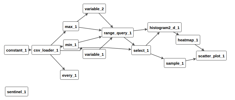
Figure 1shows the graph dependency view of the pipeline, labeled with the internal identifiers of the modules. In addition to the 2 modules created explicitly (csv_loader_1 and scatter_plot_1), we see many others created by the method create_dependent_modules. Two modules min and max progressively compute the absolute minimum and maximum values over all the columns of the dataset. The values are sent to the range_query module that will generate a range query to the select module, according to two variable modules. These modules are input modules that maintain a data frame of user-specified minimum and maximum values to implement the range selection. The two variable modules are dependent of the min or max modules—as visualized by a link in the dependency graph—through an input slot called “like” that allows the variable modules to create a data frame with the same schema as their input slots. Initially, these variable values are undefined so the range_query module generates no query and the select module does not filter any row of the data frame.
The range-query module provides a set of range-sliders for our web-based
interfaces.
As explained in
Section 3.7, the range_query module produces a
data frame with only one column called “query” that contains a
select expression such as -74.20 < pickup_longitude < -73.1.
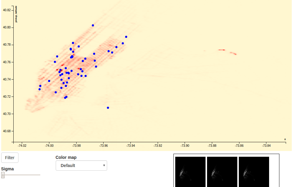
The visualization is visible on Figure 2, using a Heatmap with points overlaid. The points in that case are random samples; if a function of interest is available, the points can be chosen as the most interesting, or the most typical. The scatterplot can be explored using pan and zoom, but the resolution of the Heatmap ( bins by default) is not changed unless the “Filter” button is selected. This button also changes the range_query module to select the visible part of the display and hence increase the resolution of the Heatmap by allocating all the bins to the area of interest.
4.1 Progressive K-Means
It is important to be able to adapt well-known data analysis methods to ProgressiVis so as to provide all the building block to implement powerful systems (feature F7). K-means clustering is a classical scalable method that is well suited to a progressive implementation. The classical algorithm [22] is iterative. The variant called Mini Batch k-means [37] provides the control needed by ProgressiVis to bound the time of each run by using a stochastic update during the iterations instead of a deterministic one. The two algorithms converge to very close results [37]. This section explains some technical issues with adapting an iterative algorithm for ProgressiVis. Several iterative algorithms can be made progressive by using stochastic iterations so the principle is generalizable, although the actual implementations might differ greatly.
The classical k-means algorithm is not bounded in time because, for a data table of length :
- 1.
its inner loop runs until a numerical convergence condition is verified, not a bounded number of iterations;
- 2.
the iterative computation of the label associated with each point (the closest cluster centroid) takes time proportional to , which will grow when the data table grows;
- 3.
the centroid computations will also run in time proportional to .
The Mini Batch k-means algorithm splits the whole algorithm in mini batches, typically points, and “fixes” the cluster centroids with data from the new batches. The outer loop is run a specified number of times or stops when the convergence criteria is reached. Integrating that algorithm into ProgressiVis requires a few steps:
- 1.
deciding what algorithm unit will be mapped to one step;
- 2.
removing the unbounded iterations from the algorithm so that it complies with the
run_step()method; - 3.
handling the input and outputs correctly, in particular to avoid generating too much work for dependent modules.
We integrated the scikit-learn [31] implementation of the algorithm in ProgressiVis in a relatively straightforward way (see 5). We then extended the implementation in two ways: we added a steering capability, and we created a mechanism to compute the point labels without triggering too many recomputations.
4.1.1 Steerable K-Means
A ProgressiVis module needs to declare that it handles interaction by
returning “True” from the method is_input() and by
defining the method from_input(msg). In our case, we want
to be able to change interactively the cluster centroids, because the
k-means algorithm can become trapped in local minima and the
progressive variant is only doing one pass over the input points,
never reconsidering the initial choices it has computed for the first
input rows. The local minima problem exists for normal k-means, but
the second problem only happens with progressive (and online) k-means.
See 6 for the simplified code to implement steering.
Our scatterplot module supports dragging the cluster centroids and feeding them back to the k-means module. When a cluster center or several are moved and the new position sent to the module, a progressive recomputation is triggered with the new cluster centroids specified in the initialization. The module is responsible for providing cognitively understandable feedback [41, 25]. We tried multiple implementations of the steering and settled on re-running the algorithm from the beginning, using the interactively specified centroids as the initial configuration. Alternatively, we could have just continued the algorithm with the new centroids, but the quality seemed worse. These kinds of decisions have to be made for each steerable module, and can sometimes be left to the user for finer control.
4.1.2 Stabilizing Labeling
The k-means algorithm computes cluster positions, but can also compute the “labeling” of the input points: which cluster center is the closest to each point. This labeling should in principle be performed every time cluster centers change. Iterative algorithms such as k-means improve solutions continuously: the cluster centroids are updated at each iteration when new points arrive. Using the raw progressive computation paradigm, all the modules dependent on the cluster centroids would need to work all the time to take into account the changes and so the point labeling would be recomputed all the time. To avoid too many recomputations, a simple strategy consists in delaying the propagation until some amount of change is measured. ProgressiVis provides a module select_delta that receives a data table as input, considered as a table with multidimensional data, and propagates it as output, but only for rows that changed more than a threshold. The labeling module can then be connected to that select_delta module to recompute the labels when enough change occurred.
5 Discussion
ProgressiVis shows that typical exploratory analytics computations can be performed in a progressive way with either a script-style or a GUI-style interface. Currently ProgressiVis is organized in 9 sub-packages (core, io, stats, metrics, cluster, vis, server, and dataset). Its core is made of 27 internal classes and provides 36 modules with regression tests. It can be downloaded at https://github.com/jdfekete/progressivis.
The implementation choices in ProgressiVis are the simplest we could find to prove the feasibility of progressive analytics; we will improve these choices later when we gain more experience about progressive systems, the pitfalls of our choices, and better alternatives. For example, our scheduler does not attempt at optimizing the overall work of modules in a pipeline: a loader can be relatively slow whereas all the following modules perform their computations very quickly on the arriving data, never using their whole quantum. A smart scheduler could allocate more time to the loader and less to the other modules so as to comply with a total expected iteration time. Currently, our scheduler just obeys to the modules quantum, except in the transient interactive mode. Since the quantum is a tunable parameter of each module, we rely on analysts to change it interactively at runtime according to their preference.
ProgressiVis focuses on the implementation of the mechanisms needed to run progressive programs. User requirements from HCI such as providing progress-bars or convergence/quality information (feature F2) are not implemented yet or not consistently, mainly because more work is needed to understand the whole set of extra information required to fulfill the HCI and cognitive requirements, and the way the information should be provided.
ProgressiVis is scalable, but remains within the capabilities and limits of its implementation in Python. Still, it delivers progressive results at a human-processable speed, using effectively the main memory and CPU. With modern computer architectures using multiple cache levels and solid-state disks, the virtual memory of a laptop can reach and the processing speed depends mostly on cache prediction; see [4] for a discussion about main memory and what it has become in the era of multiple cache levels. ProgressiVis can perform progressive computations efficiently, but there will always be an overhead for progressiveness due to the requirement to generate intermediate results. Still we were surprised when running regression tests of ProgressiVis against the standard Python/NumPy implementations to realize that allocating memory in a progressive manner seems to suit the operating system better than by large chunks that sometimes make it “freeze” for a minute. More tests are required to understand if that behavior is exceptional or frequent.
The current Python implementation suffers from shortcomings of the standard libraries. For example, the SciPy library offers functions to compute the largest eigenvector/eigenvalues of a matrix using an iterative solver, essential for e.g. computing a PCA progressively. However, these functions are black-boxes and do not expose their iterations. Offering lower-level functions to control the iterations would spare ProgressiVis from reimplementing them. The same is true for algorithms provided by other Python libraries such as Pandas and scikit-learn. We understand that libraries and new computation paradigms co-evolve so, to address these issues in the future, we need to advertise ProgressiVis to explain our requirements and convince library authors to better support the needs of progressive systems.
6 Conclusion and Future Work
This article presented the progressive analytics computation paradigm and its experimental implementation ProgressiVis. We introduced the paradigm, defined it formally and contrasted it with related concepts. We then described the implementation of the experimental ProgressiVis toolkit, meant to support the development of progressive systems; it can be used to explore data using a command-line interface and web-based interactive visualizations. Through examples, we showed how to explore data with progressive analytics.
In the near future, we want to extend our implementation to become a fully usable system and toolkit for scalable analytics. In particular, we want to provide a rich set of progressive analytical modules by devising strategies to adapt families of algorithms to our progressive computation paradigm. For example, while implementing computation modules, we found multiple possible strategies to turn online and iterative algorithms progressive, using hybrid solutions such as running the main algorithm in a parallel thread and returning predictions between long iterations. We also want to further explore how standard visualization techniques can be adapted for progressiveness.
In the forthcoming years, we will explore the multiple new research questions raised by the progressive analytics computation paradigm on algorithms, machine-learning, cognition, HCI, visualization, visual analytics, databases, and distributed computing.
Acknowledgements.
This work has been conducted during my Sabbatical at NYU-Poly in the Visualization and Data Analytics (ViDA) group, partially funded by the Center for Data Science at NYU. Thanks to Juliana Freire for the fruitful feedback she provided me, to Marie Douriez for her help in implementing and experimenting Progressive MDS, and to Andreas Müller for his advises on Scikit-Learn.References
- [1] S. Agarwal, B. Mozafari, A. Panda, H. Milner, S. Madden, and I. Stoica. BlinkDB: Queries with bounded errors and bounded response times on very large data. In Proc. of the 8th ACM European Conference on Computer Systems, EuroSys ’13, pages 29–42. ACM, 2013.
- [2] D. Auber. Graph Drawing Software, chapter Tulip — A Huge Graph Visualization Framework, pages 105–126. Springer, 2004.
- [3] J. Ayres, J. Flannick, J. Gehrke, and T. Yiu. Sequential pattern mining using a bitmap representation. In Proc. of the Eighth ACM SIGKDD International Conference on Knowledge Discovery and Data Mining, KDD ’02, pages 429–435. ACM, 2002.
- [4] P. A. Boncz, M. L. Kersten, and S. Manegold. Breaking the memory wall in monetdb. Commun. ACM, 51(12):77–85, Dec. 2008.
- [5] A. Borodin and R. El-Yaniv. Online Computation and Competitive Analysis. Cambridge University Press, 1998.
- [6] M. Bostock, V. Ogievetsky, and J. Heer. D3 data-driven documents. IEEE Trans. Vis. Comput. Graphics, 17(12):2301–2309, Dec. 2011.
- [7] J. Choo, C. Lee, H. Kim, H. Lee, C. Reddy, B. Drake, and H. Park. Pive: Per-iteration visualization environment for supporting real-time interactions with computational methods. In Visual Analytics Science and Technology (VAST), 2014 IEEE Conference on, pages 241–242, Oct 2014.
- [8] A. Crotty, A. Galakatos, E. Zgraggen, C. Binnig, and T. Kraska. Vizdom: Interactive analytics through pen and touch. Proc. VLDB Endow., 8(12):2024–2027, Aug. 2015.
- [9] R. DeLine, D. Fisher, B. Chandramouli, J. Goldstein, M. Barnett, J. Terwilliger, and J. Wernsing. Tempe: Live scripting for live data. In Visual Languages and Human-Centric Computing (VL/HCC), IEEE Symposium on, pages 137–141, Oct 2015.
- [10] N. Diakopoulos, S. Cass, and J. Romero. Data-driven rankings: The design and development of the ieee top programming languages news app. IEEE Spectrum, July 2015.
- [11] J.-D. Fekete. ProgressiVis: a Toolkit for Steerable Progressive Analytics and Visualization. In 1st Workshop on Data Systems for Interactive Analysis, Oct. 2015.
- [12] D. Fisher, I. Popov, S. Drucker, and M. Schraefel. Trust me, i’m partially right: incremental visualization lets analysts explore large datasets faster. In CHI ’12, pages 1673–1682, 2012.
- [13] M. Glueck, A. Khan, and D. J. Wigdor. Dive in!: Enabling progressive loading for real-time navigation of data visualizations. In Proc. of the SIGCHI Conf. on Human Factors in Comp. Sys., CHI ’14, pages 561–570. ACM, 2014.
- [14] C. Harrison, Z. Yeo, and S. E. Hudson. Faster progress bars: Manipulating perceived duration with visual augmentations. In Proc. of the SIGCHI Conf. on Human Factors in Comp. Sys., CHI ’10, pages 1545–1548. ACM, 2010.
- [15] J. M. Hellerstein, P. J. Haas, and H. J. Wang. Online aggregation. In Proc. of the 1997 ACM SIGMOD International Conference on Management of Data, SIGMOD ’97, pages 171–182. ACM, 1997.
- [16] E. Jones, T. Oliphant, P. Peterson, et al. SciPy: Open source scientific tools for Python, 2001–. [Online; accessed 2016-03-11].
- [17] M. L. Kersten, S. Idreos, S. Manegold, and E. Liarou. The researcher’s guide to the data deluge: Querying a scientific database in just a few seconds. PVLDB, 4(12):1474–1477, 2011.
- [18] B. Li, Y. Diao, and P. Shenoy. Supporting scalable analytics with latency constraints. Proc. VLDB Endow., 8(11):1166–1177, July 2015.
- [19] L. Lins, J. T. Klosowski, and C. Scheidegger. Nanocubes for real-time exploration of spatiotemporal datasets. IEEE Trans. Vis. Comput. Graphics, 19(12):2456–2465, Dec 2013.
- [20] Z. Liu and J. Heer. The effects of interactive latency on exploratory visual analysis. IEEE Trans. Vis. Comput. Graphics, 20(12):2122–2131, Dec 2014.
- [21] K.-L. Ma. In Situ Visualization at Extreme Scale: Challenges and Opportunities. IEEE Comput. Graph. Appl. Mag, 29(6):14–19, Nov 2009.
- [22] J. MacQueen. Some methods for classification and analysis of multivariate observations. In Proc. of the Fifth Berkeley Symposium on Mathematical Statistics and Probability, volume 1: Statistics, pages 281–297. University of California Press, Berkeley, Calif., 1967.
- [23] W. McKinney. pandas: a foundational python library for data analysis and statistics. Python for High Performance and Scientific Computing, pages 1–9, 2011.
- [24] R. B. Miller. Response time in man-computer conversational transactions. In Proc. of the Fall Joint Computer Conference, Part I, pages 267–277. ACM, 1968.
- [25] T. Mühlbacher, H. Piringer, S. Gratzl, M. Sedlmair, and M. Streit. Opening the black box: Strategies for increased user involvement in existing algorithm implementations. IEEE Trans. Vis. Comput. Graphics, 20(12):1643–1652, Dec 2014.
- [26] J. D. Mulder, J. J. van Wijk, and R. van Liere. A survey of computational steering environments. Future Gener. Comput. Syst., 15(1):119–129, Feb. 1999.
- [27] S. Muthukrishnan. Data streams: Algorithms and applications. Found. Trends Theor. Comput. Sci., 1(2):117–236, Aug. 2005.
- [28] B. A. Myers. The importance of percent-done progress indicators for computer-human interfaces. In Proc. of the SIGCHI Conf. on Human Factors in Comp. Sys., CHI ’85, pages 11–17. ACM, 1985.
- [29] J. Nielsen. Usability engineering. Elsevier, 1994.
- [30] J. Nielsen. Response times: The 3 important limits. https://www.nngroup.com/articles/response-times-3-important-limits/, Mar. 2016.
- [31] F. Pedregosa, G. Varoquaux, A. Gramfort, V. Michel, B. Thirion, O. Grisel, M. Blondel, P. Prettenhofer, R. Weiss, V. Dubourg, J. Vanderplas, A. Passos, D. Cournapeau, M. Brucher, M. Perrot, and E. Duchesnay. Scikit-learn: Machine learning in Python. Journal of Machine Learning Research, 12:2825–2830, 2011.
- [32] N. Pentreath. Machine Learning with Spark. Community experience distilled. Packt Publishing, 2015.
- [33] N. Pezzotti, B. P. F. Lelieveldt, L. van der Maaten, T. Höllt, E. Eisemann, and A. Vilanova. Approximated and user steerable tsne for progressive visual analytics. CoRR, abs/1512.01655, 2015.
- [34] R Core Team. R: A Language and Environment for Statistical Computing. R Foundation for Statistical Computing, 2013. ISBN 3-900051-07-0.
- [35] Y. Saad. Iterative methods for sparse linear systems. Siam, 2003.
- [36] H.-J. Schulz, M. Angelini, G. Santucci, and H. Schumann. An enhanced visualization process model for incremental visualization. IEEE Trans. Vis. Comput. Graphics, PP(99):1–1, 2015.
- [37] D. Sculley. Web-scale k-means clustering. In Proc. of the 19th International Conference on World Wide Web, WWW ’10, pages 1177–1178. ACM, 2010.
- [38] S. C. Seow. Designing and Engineering Time: The Psychology of Time Perception in Software. Addison-Wesley Professional, 2008.
- [39] B. Shneiderman. Direct manipulation: A step beyond programming languages. Computer, 16(8):57–69, Aug 1983.
- [40] B. Shneiderman. Response time and display rate in human performance with computers. ACM Comput. Surv., 16(3):265–285, Sept. 1984.
- [41] C. D. Stolper, A. Perer, and D. Gotz. Progressive visual analytics: User-driven visual exploration of in-progress analytics. IEEE Trans. Vis. Comput. Graphics, 20(12):1653–1662, Dec 2014.
- [42] S. van der Walt, S. C. Colbert, and G. Varoquaux. The numpy array: A structure for efficient numerical computation. Computing in Science Engineering, 13(2):22–30, March 2011.
- [43] M. Williams and T. Munzner. Steerable, progressive multidimensional scaling. In Information Visualization, 2004. INFOVIS 2004. IEEE Symposium on, pages 57–64, 2004.
- [44] M. Zaharia, M. Chowdhury, M. J. Franklin, S. Shenker, and I. Stoica. Spark: Cluster computing with working sets. In Proc. of the 2Nd USENIX Conference on Hot Topics in Cloud Computing, HotCloud’10, pages 10–10. USENIX Association, 2010.
- [45] M. Zaharia, T. Das, H. Li, T. Hunter, S. Shenker, and I. Stoica. Discretized streams: Fault-tolerant streaming computation at scale. In Proc. of the Twenty-Fourth ACM Symposium on Operating Systems Principles, SOSP ’13, pages 423–438. ACM, 2013.