From Planck data to Planck era:
Observational tests of Holographic Cosmology

Observations of the cosmic microwave background (CMB) offer a unique window into the very early Universe and Planck scale physics. The standard model of cosmology, the so-called $\Lambda$CDM model, provides an excellent fit to observational data with just six parameter. Four of these parameters describe the composition and evolution of the Universe, while the other two are linked with the physics of the very early Universe. These two parameters, the tilt $n_{s}$ and and the amplitude $\Delta^{2}_{0}(q_{*})$, parameterize the power spectrum of primordial curvature perturbations,

where $q_{*}$, the pivot, is an an arbitrary reference scale. This form of the power spectrum is a good approximation for slow-roll inflationary models and has the ability to fit the CMB data well. Indeed, a near-power-law scalar power spectrum may be considered as a success of the theory of cosmic inflation.

The theory of inflation is an effective theory. It is based on gravity coupled to (appropriate) matter perturbatively quantized around an accelarating FLRW background. At sufficiently early times the curvature of the FLRW spacetime becomes large and the perturbative treatment is expected to break down – in this regime we would need a full-fledged theory of quantum gravity. One of the deepest insights about quantum gravity that emerged in recent times is that it is expected to be holographic [1, 2, 3], meaning that there should be an equivalent description of the bulk physics using a quantum field theory with no gravity in one dimension less. One may thus seek to use holography to model the very early Universe.

Holographic dualities were originally developed for spacetimes with negative cosmological constant (the AdS/CFT duality) [3] and soon afterwards the extension to de Sitter and cosmology was considered [4, 5, 6, 7, 8]. In this context, the statement of the duality is that the partition function of the dual QFT computes the wavefunction of the universe [8] and using this wavefunction cosmological observables may be obtained. Alternatively, [9, 10, 11, 12, 13], one may use the Domain-wall/Cosmology correspondence [14]. The two approaches are equivalent [15].

Holography offers a new framework that can accommodate conventional inflation but also leads to qualitatively new models for the very early universe. While conventional inflation corresponds to a strongly coupled QFT [16, 17, 18, 19, 20, 21, 22, 23, 24, 25, 26, 27, 28, 29, 30, 31, 32], the new models are associated with a weakly coupled QFT. These models correspond to a non-geometric bulk, and yet holography allows us to compute the predictions for the cosmological observables. We emphasise that the application of holography to cosmology is conjectural, the theoretical validity of such dualities is still open and different authors approach the topic in different ways. Here we seek to test these ideas against observations.

A class of non-geometric models were introduced in [9] and their prediction have been worked out in [9, 10, 11, 12, 13, 33, 34]. These models are based on three dimensional super-renormalizable QFT and they universally predict a scalar power spectrum of the form,

where $g$ is related to the coupling constant of the dual QFT, while $\beta$ depends on the parameters of the dual QFT (see below).

The form of the power spectrum in (2) is distinctly different from (1)¹¹ 1 For small enough $g$, one may rewrite (2) in the form (1) with momentum dependent $n_{s}(q)$. However, as discussed [9, 35], the momentum dependence of $n_{s}(q)$ is qualitatively different from that of slow-roll inflationary models [36].. Since these are qualitatively different parametrizations, one may ask which of the two is preferred by the data. Note that this question is a priori independent of the underlying physical models that produced (1) and (2). This question has already been addressed for WMAP7 data [37] in [35, 38] and it was found that while the data mildly favour $\Lambda$CDM, it was insufficient to definitively discriminate between the two cases. Since then, the Planck mission has released its data [39] and it is now time to revisit this issue. We will present the main conclusions of the fit to Planck data here, referring to [40] for a more detailed discussion.

On the theoretical side, there has also been significant progress since [35]. While the form of (2) is universally fixed, the precise relation between $g$ and $\beta$ and the parameters of the dual QFT requires a 2-loop computation, which has now been carried out in [41]. We can thus not only check whether (2) is compatible with CMB data, but also use the data to do a model selection.

Theory.— Following [9], we consider the dual QFT to be $SU(N)$ gauge theory coupled to scalars $\Phi^{M}$ and fermions $\psi^{L}$, where $M,L$ are flavor indices. The action is given by

where all fields, $\varphi=\varphi^{a}T^{a}$, are in the adjoint of $SU(N)$ and $\mathrm{tr}T^{a}T^{b}=\frac{1}{2}\delta^{ab}$. $F_{ij}$ is the Yang-Mills field strength, and $\mathcal{D}$ is a gauge covariant derivative. We use the shorthand notation $(\mathcal{D}\Phi)^{2}=\delta_{M_{1}M_{2}}\mathcal{D}_{i}\Phi^{M_{1}}\mathcal{D}^{i}\Phi^{M_{2}}$, $\bar{\psi}\mathcal{D}\!\!\!\!/\ \!\psi=\delta_{L_{1}L_{2}}\bar{\psi}^{L_{1}}\gamma^{i}\mathcal{D}_{i}\psi^{L_{2}}$, $\mu\cdot(\Phi\bar{\psi}\psi)\equiv\mu_{ML_{1}L_{2}}\Phi^{M}\bar{\psi}^{L_{1}}\psi^{L_{2}}$ and $\lambda\cdot\Phi^{4}\equiv\lambda_{M_{1}M_{2}M_{3}M_{4}}\Phi^{M_{1}}\Phi^{M_{2}}\Phi^{M_{3}}\Phi^{M_{4}}$.

The holographic dictionary relates the scalar and tensor power spectra to the 2-point function of the energy-momentum tensor $T_{ij}$. For the scalar power spectrum,

where $g_{\mathrm{eff}}^{2}(q)\equiv g_{\mathrm{YM}}^{2}N/q$ is the effective dimensionless ’t Hooft coupling constant, $q$ is the magnitude of the momentum $\vec{q}$ and $f(g_{\mathrm{eff}}^{2})$ is extracted from the momentum space 2-point of function of the trace of the energy momentum tensor, $\langle T^{i}_{i}(\vec{p})T^{j}_{j}(\vec{q})\rangle=(2\pi)^{3}\delta(\vec{p}+\vec{q})q^{3}N^{2}f(g_{\mathrm{eff}}^{2})$. In perturbation theory,

The function $f_{0}$ is determined by a 1-loop computation, while $f_{1}$ and $f_{2}$ come from 2-loops. The presence of the logarithm is due to UV and IR divergences in the computation of the 2-point function of the energy momentum tensor. A detailed derivation of (4) may be found in [10, 35]. Following [35], (2) and (4-5) match if:

So, a universal prediction of these class of theories is the power spectrum (2), independent of the details of the 2-loop computation²² 2 This assumes $f_{1}\neq 0$. A separate analysis is required, where $f_{1}=0$, e.g., for (3) without gauge fields and fermions. .

The 1-loop computation was done in [9, 10] and we here report the result of the 2-loop computation [41] – a summary of the computation is provided in the appendix.. The final result is

where $\mathcal{N}_{\Phi}$ and $\mathcal{N}_{\psi}$ are the total number of scalars and fermions, and

where $\mu_{M_{1}M_{2}}^{2}=\sum_{L_{1},L_{2}}\mu_{M_{1}L_{1}L_{2}}\mu_{M_{2}L_{2}L_{1}}$, $\xi_{M}$ is the non-minimality parameter³³ 3 Non-minimal scalars on a curved background have the coupling $1/(2g_{\mathrm{YM}}^{2})\sum_{M}\int\xi_{M}R(\Phi^{M})^{2}$, where $R$ is the curvature scalar, and this term induces an “improvement term” to their energy momentum tensor, $T_{ij}=(2/\sqrt{g})(\delta S/\delta g^{ij})|_{g_{ij}=\delta_{ij}}$, see [42]. and summations over $M(L)$ are over scalars (fermions).

Fitting to data.— We would like now to assess how well a power spectrum of the form (2) fits the cosmological data and compare with that of the conventional power-law power spectrum. Recall that $\Lambda$CDM is parametrized by six parameters, $(\Omega_{b}h^{2},\Omega_{c}h^{2},\theta,\tau,\Delta_{0}^{2},n_{s})$, where $\Omega_{b}h^{2}$ and $\Omega_{c}h^{2}$ are the baryon and dark matter densities, $\theta$ is the angular size of the sound horizon at recombination, $\tau$ is the the optical depth due to re-ionization and $\Delta_{0}^{2}$, $n_{s}$ are the parameters entering in (1). To formalize the comparison, we define (following [35]) holographic cosmology (HC) as the model parametrized by $(\Omega_{b}h^{2},\Omega_{c}h^{2},\theta,\tau,\Delta_{0}^{2},g,\ln\beta)$⁴⁴ 4 In [35] the parameter $\beta$ was incorrectly assumed to be equal one. We refitted the WMAP data and found that the global minimum is at $\beta=3.777$.. This model has 7 parameters so in order to compare models with the same number of parameters we also consider $\Lambda$CDM with running $\alpha_{s}=dn_{s}/d\ln q$. Note that our aim here is to compare empirical models, not the underlying physical models that lead to them. If the data selects one of the two empirical models, then this would falsify all physical models that underlie the other model.

We analysed the data using CosmoMC [43, 44, 45, 46, 47, 48, 49]. We ran both $\Lambda$CDM and HC with the same datasets, fitting the models to the Planck 2015 data including lensing [39, 50, 51, 52, 53, 54, 55], as well as Baryonic Acoustic Oscillations (BAO) [56, 57, 58, 59, 60, 61, 62, 63] and BICEP2-Keck-Planck (BKP) polarization [64]. After CosmoMC had run to determine the mean and errors in the parameters, we ran the minimizer [65] within the code to determine the best fit parameters and likelihood.

The Planck angular TT spectrum together with the best fit curves and residuals for HC and $\Lambda$CDM are presented in Fig. 1. Notice that the difference between $\Lambda$CDM and HC lies within the 68% region of Planck, with the largest difference being at small multipoles. Very similar results hold for the TE and EE spectra [40]. We determined the best fit values for all parameters for HC, $\Lambda$CDM and $\Lambda$CDM with running. Our values for the parameters of $\Lambda$CDM and $\Lambda$CDM with running are in agreement with those determined by the Planck team. All common parameters of the three models are within $1\sigma$ of each other (with the notable exception of the optical depth $\tau$ [40]). We report the values of $\Delta_{0},g,\ln\beta$ and $\chi^{2}$ in Table 1 (the list of all parameters can be found in [40]). The $\chi^{2}$ of the fit indicates that HC is disfavoured at about 2.2$\sigma$ relative to $\Lambda$CDM with running, when we consider all multipoles.

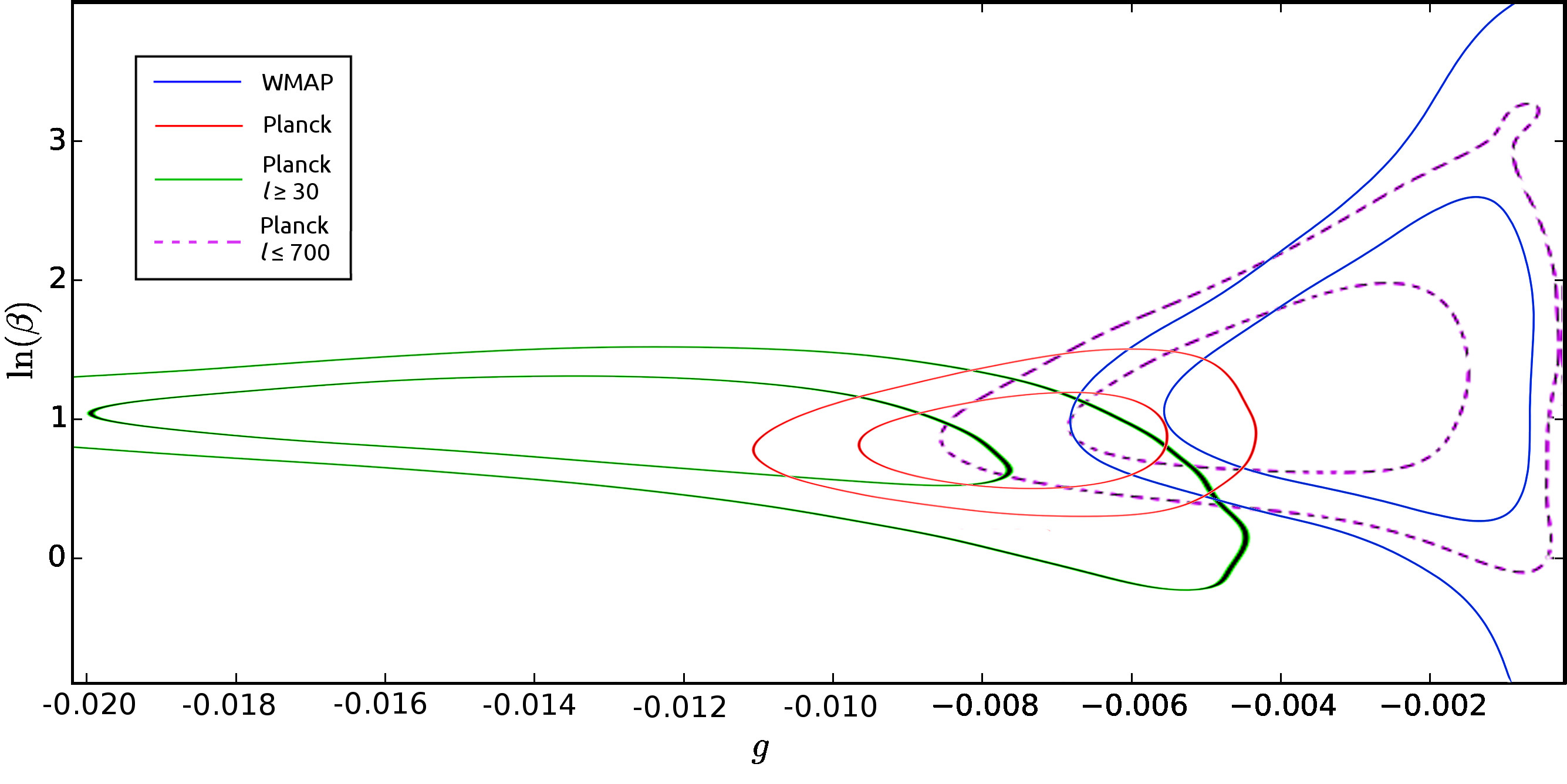
Relative to the WMAP fit in [35] the value of $g$ has decreased from $-1.3\times 10^{-3}$ to $-7\times 10^{-3}$. In Fig. 2, we investigate how the value of $g$ changes if we change the range of multipoles that we consider. It is clear from the plot that the value of $g$ is compatible between WMAP and Planck, if we keep the same multipoles. It is also clear that the high $l$ modes want to push $g$ to lower negative values. Larger values of $|g|$ indicate that the theory may become non-perturbative at very low $l$ and, as such, the predictions of the model cannot be trusted in that regime. We shall see below that this is supported by model selection criteria. Therefore, we repeat the fitting, excluding the $l<30$ multipoles. The results for $\Delta_{0},g,\ln\beta$ and $\chi^{2}$ are tabulated in Table 1. With this data, all common parameters are now compatible with each other [40]. The $\chi^{2}$ test shows that the three models are now within $1\sigma$.

The power spectrum for the tensors takes the same form as (2) but with different values of $g$ and $\beta$. We fitted the data with this form of the power spectrum and found that it is consistent with $r=0$; the $2\sigma$ upper limit on the tensor-to-scalar ratio is $r<0.125$.

Bayesian Evidence.— In comparing different models, one often uses information criteria such as the value of $\chi^{2}$, which quantifies the goodness of a fit. We emphasise that with “model” we mean the three empirical models introduced above, $\Lambda$CDM, $\Lambda$CDM with running and HC. What we really want to know, however, is what is the probability for each of these models given the data. This is obtained by computing the Bayesian Evidence.

As discussed in [35], if we assume flat priors for all parameters $\alpha_{M}$ that define a given model, the Bayesian evidence is given by $E=\frac{1}{{\rm Vol}_{M}}\int d\alpha_{M}\mathcal{L\left(\alpha_{M}\right)}$, where $\mathcal{L\left(\alpha_{M}\right)}$ is the likelihood and Vol_M is the volume of the region in parameter space over which the prior probability distribution is non-zero. The evidence may be computed either by using CosmoMC or by MultiNest [66, 67, 68].

Note that the aim here is to compare empirical models and we determined the priors from previous fits of the same empirical models to data (as is common)⁵⁵ 5 Had we focused on specific physical models we could use the wavefunction of the universe to obtain corresponding theoretical priors, see [18] for work in this direction.. We use the priors in Table 4 of [35], except that the upper limit of $100\,\theta$ is taken to be 1.05. The prior for the running is taken to be $|\alpha_{s}|\leq 0.05$. The priors for $n_{s}$ are the asymmetric prior used in [35]: $0.92\leq n_{s}\leq 1$. For the prior for $g$ we use variable range, $g_{\rm min}\leq g<0$. This prior is fixed by the requirement that perturbation theory is valid. We will allow for the possibility that the perturbative expansion is valid only for $l>30$. We use as a rough estimate for the validity of perturbation theory that $gq^{*}/q$ is sufficiently small, taking this to mean a value between 0.20 and 1 at $l=30$⁶⁶ 6 The momenta and multipoles are related via $q=l/r_{h}$, where $r_{h}=14.2$ Gpc is the comoving radius of the last scattering surface.. This translates into $-0.009<g_{\rm min}<-0.45$. The prior for $\beta$ is fixed by using the results from (our fit to) WMAP data. We use two sets of priors: one coming from the 1$\sigma$ range ($0\leq\ln\beta\leq 2$) and the other from the 2$\sigma$ range ($-0.2\leq\ln\beta\leq 3.5$).

The results for the Bayesian evidence are presented in Fig. 3 for $l\geq 30$, where 2-loop predictions (2) can be trusted. As a guide [69], a difference $\ln E<1$ is insignificant and $2.5<\ln E<5$ is strongly significant. We see that the difference between evidence for $\Lambda$CDM and HC predictions is insignificant, with marginal preference for HC, depending on the choice of priors.

Model selection.— We would like now to examine whether we can use the data to rule out or in some of the models described by (3). There are phenomenological and theoretical constraints that we need to satisfy. The phenomenological constraints are: the bound on the tensor-to-scalar ratio, $r\leq 0.125$, should be satisfied, and the model should reproduce the observed values for the amplitude $\Delta_{0}^{2}$ and $\ln\beta$. The theoretical prediction for the $r$ is [9, 10, 34],

and the theoretical predictions for $\Delta_{0}^{2}$ and $\ln\beta$ are given in (6-9). In deriving (2) we used a ’t Hooft large $N$ expansion and perturbation theory in $g_{\mathrm{eff}}^{2}$. We thus need to check that any solution of the phenomenological constraints is consistent with these theoretical assumptions.

There are a few universal properties of the 2-loop correction, $gq_{*}/q\ln|q/\beta gq_{*}|$. This term vanishes at large $q$, reflecting the fact that the QFTs we consider are superrenormalizable. Its absolute value gradually increases till it reaches the local maximum $1/e\beta$ at $q=e\beta|g|q_{*}$. At lower values of $l$ the 2-loop term changes sign and grows very fast as we go to lower multipoles becoming equal to one (same size as the 1-loop contribution) below $l=10$. Therefore, we should not trust these models below $l\sim 10$. In fact, one should even be cautious in using the 2-loop approximation for $l$’s lower than 35. While the overall magnitude of the 2-loop term is small up until $l=10$ this happens due to large cancellation between the $f_{1}$ and the $f_{2}$ term in (5). We will use as an indicator of the reliability of perturbation theory the size of $f_{1}g_{\mathrm{eff}}^{2}\ln g_{\mathrm{eff}}^{2}$.

Let us consider gauge theory coupled to a large number, $\mathcal{N}_{\Phi}$, of non-mimimal scalars, all with the same non-minimality parameter $\xi$ and the same quartic coupling $\lambda$. For sufficiently large $\mathcal{N}_{\Phi}$, the scalar-to-tensor ratio (10) becomes

and the bound on $r$ implies, $|1-8\xi|\leq 0.061$, where the equality holds when $r=0.12.$ Choosing a value of $\xi$, then the observational values of $\Delta_{0}^{2}$ and $\ln\beta$ give two equations, which can always be solved to determine $N$ and $\mathcal{N}_{\Phi}$. For example, if we choose $\xi=0.133$, which correspond to $r=0.12$, and take $\lambda=1$ the solution to the two constraints is

This solution satisfies the theoretical constraints: firstly, $N^{2}\gg\mathcal{N}_{\Phi}$, so the large $N$ expansion is justified and secondly, the effective coupling remains small for all momenta seen by Planck, $3.3\times 10^{-4}\leq g_{\mathrm{eff}}^{2}(q)\leq 0.41$. For this solution however $f_{1}\approx-8(1-48\xi^{2})/(1-8\xi)^{2}\approx-11$ and $f_{1}g_{\mathrm{eff}}^{2}\ln g_{\mathrm{eff}}^{2}\approx 1$ when $l=35$, so we should not trust the perturbative expansion below around $l\approx 35$.

Conclusions.— We showed that holographic models based on three-dimensional perturbative QFT are capable of explaining the CMB data and are competitive to $\Lambda$CDM model. However, at very low multipoles (roughly $l<30$), the perturbative expansion breaks down and in this regime the prediction of the theory cannot be trusted. The data are consistent with the dual theory being gauge theory coupled to a large number of nearly conformal scalars with a quartic interaction. It would be interesting to further analyze these models in order to extract other properties that may be testable against observations. In particular, non-perturbative methods (such as putting the dual QFT on a lattice) can be used to reliably model the very low multipoles, which may potentially explain the apparent large angle anomalies in the CMB sky (e.g., [70]).

References

- [1] G. ’t Hooft, in Salamfest 1993:0284-296 (1993) pp. 0284–296, arXiv:gr-qc/9310026 [gr-qc] .
- [2] L. Susskind, J. Math. Phys. 36, 6377 (1995), arXiv:hep-th/9409089 [hep-th] .
- [3] J. M. Maldacena, Int. J. Theor. Phys. 38, 1113 (1999), [Adv. Theor. Math. Phys.2,231(1998)], arXiv:hep-th/9711200 [hep-th] .
- [4] C. M. Hull, JHEP 07, 021 (1998), arXiv:hep-th/9806146 [hep-th] .
- [5] E. Witten, in Strings 2001: International Conference Mumbai, India, January 5-10, 2001 (2001) arXiv:hep-th/0106109 [hep-th] .
- [6] A. Strominger, JHEP 10, 034 (2001a), arXiv:hep-th/0106113 [hep-th] .
- [7] A. Strominger, JHEP 11, 049 (2001b), arXiv:hep-th/0110087 [hep-th] .
- [8] J. M. Maldacena, JHEP 05, 013 (2003), arXiv:astro-ph/0210603 [astro-ph] .
- [9] P. McFadden and K. Skenderis, Phys. Rev. D81, 021301 (2010a), arXiv:0907.5542 [hep-th] .
- [10] P. McFadden and K. Skenderis, Classical and quantum gravity. Proceedings, 1st Mediterranean Conference, MCCQG 2009, Kolymbari, Crete, Greece, September 14-18, 2009, J. Phys. Conf. Ser. 222, 012007 (2010b), arXiv:1001.2007 [hep-th] .
- [11] P. McFadden and K. Skenderis, JCAP 1105, 013 (2011a), arXiv:1011.0452 [hep-th] .
- [12] P. McFadden and K. Skenderis, JCAP 1106, 030 (2011b), arXiv:1104.3894 [hep-th] .
- [13] A. Bzowski, P. McFadden, and K. Skenderis, JHEP 03, 091 (2012), arXiv:1112.1967 [hep-th] .
- [14] K. Skenderis and P. K. Townsend, Phys. Rev. Lett. 96, 191301 (2006), arXiv:hep-th/0602260 [hep-th] .
- [15] J. Garriga, K. Skenderis, and Y. Urakawa, JCAP 1501, 028 (2015), arXiv:1410.3290 [hep-th] .
- [16] J. M. Maldacena and G. L. Pimentel, JHEP 09, 045 (2011), arXiv:1104.2846 [hep-th] .
- [17] J. B. Hartle, S. W. Hawking, and T. Hertog, (2012), arXiv:1205.3807 [hep-th] .
- [18] J. B. Hartle, S. W. Hawking, and T. Hertog, JCAP 1401, 015 (2014), arXiv:1207.6653 [hep-th] .
- [19] K. Schalm, G. Shiu, and T. van der Aalst, JCAP 1303, 005 (2013), arXiv:1211.2157 [hep-th] .
- [20] A. Bzowski, P. McFadden, and K. Skenderis, JHEP 04, 047 (2013), arXiv:1211.4550 [hep-th] .
- [21] I. Mata, S. Raju, and S. Trivedi, JHEP 07, 015 (2013), arXiv:1211.5482 [hep-th] .
- [22] J. Garriga and Y. Urakawa, JCAP 1307, 033 (2013), arXiv:1303.5997 [hep-th] .
- [23] P. McFadden, JHEP 10, 071 (2013), arXiv:1308.0331 [hep-th] .
- [24] A. Ghosh, N. Kundu, S. Raju, and S. P. Trivedi, JHEP 07, 011 (2014), arXiv:1401.1426 [hep-th] .
- [25] J. Garriga and Y. Urakawa, JHEP 06, 086 (2014), arXiv:1403.5497 [hep-th] .
- [26] N. Kundu, A. Shukla, and S. P. Trivedi, JHEP 04, 061 (2015), arXiv:1410.2606 [hep-th] .
- [27] P. McFadden, JHEP 02, 053 (2015), arXiv:1412.1874 [hep-th] .
- [28] N. Arkani-Hamed and J. Maldacena, (2015), arXiv:1503.08043 [hep-th] .
- [29] N. Kundu, A. Shukla, and S. P. Trivedi, JHEP 01, 046 (2016), arXiv:1507.06017 [hep-th] .
- [30] T. Hertog and E. van der Woerd, JCAP 1602, 010 (2016), arXiv:1509.03291 [hep-th] .
- [31] J. Garriga, Y. Urakawa, and F. Vernizzi, JCAP 1602, 036 (2016), arXiv:1509.07339 [hep-th] .
- [32] J. Garriga and Y. Urakawa, (2016), arXiv:1606.04767 [hep-th] .
- [33] C. Corianò, L. Delle Rose, and M. Serino, JHEP 12, 090 (2012), arXiv:1210.0136 [hep-th] .
- [34] S. Kawai and Y. Nakayama, JHEP 06, 052 (2014), arXiv:1403.6220 [hep-th] .
- [35] R. Easther, R. Flauger, P. McFadden, and K. Skenderis, JCAP 1109, 030 (2011), arXiv:1104.2040 [astro-ph.CO] .
- [36] A. Kosowsky and M. S. Turner, Phys. Rev. D52, 1739 (1995), arXiv:astro-ph/9504071 [astro-ph] .
- [37] E. Komatsu et al. (WMAP), Astrophys. J. Suppl. 192, 18 (2011), arXiv:1001.4538 [astro-ph.CO] .
- [38] M. Dias, Phys. Rev. D84, 023512 (2011), arXiv:1104.0625 [astro-ph.CO] .
- [39] P. A. R. Ade et al. (Planck), (2015a), arXiv:1502.01589 [astro-ph.CO] .
- [40] N. Afshordi, E. Gould, and K. Skenderis, (2016), to appear .
- [41] C. Corianò, L. Delle Rose, and K. Skenderis, (2016), to appear .
- [42] See Supplemental Material at [URL will be inserted by publisher] for technical details.
- [43] U. Seljak and M. Zaldarriaga, Astrophys. J. 469, 437 (1996), astro-ph/9603033 .
- [44] M. Zaldarriaga, U. Seljak, and E. Bertschinger, Astrophys.J. 494, 491 (1998), arXiv:astro-ph/9704265 [astro-ph] .
- [45] A. Lewis, A. Challinor, and A. Lasenby, Astrophys. J. 538, 473 (2000), arXiv:astro-ph/9911177 [astro-ph] .
- [46] A. Lewis and S. Bridle, Phys. Rev. D66, 103511 (2002), arXiv:astro-ph/0205436 [astro-ph] .
- [47] C. Howlett, A. Lewis, A. Hall, and A. Challinor, JCAP 1204, 027 (2012), arXiv:1201.3654 [astro-ph.CO] .
- [48] A. Lewis, Phys. Rev. D87, 103529 (2013), arXiv:1304.4473 [astro-ph.CO] .
- [49] A. Lewis, “CAMB Notes,” http://cosmologist.info/notes/CAMB.pdf.
- [50] P. Ade et al. (Planck), (2015b), arXiv:1502.01591 [astro-ph.CO] .
- [51] N. Aghanim et al. (Planck), (2015), arXiv:1507.02704 [astro-ph.CO] .
- [52] P. Ade et al. (Planck), (2015c), arXiv:1502.01597 [astro-ph.CO] .
- [53] C. Bennett et al. (WMAP), Astrophys.J.Suppl. 208, 20 (2013), arXiv:1212.5225 [astro-ph.CO] .
- [54] C. Reichardt, L. Shaw, O. Zahn, K. Aird, B. Benson, et al., Astrophys.J. 755, 70 (2012), arXiv:1111.0932 [astro-ph.CO] .
- [55] S. Das, T. Louis, M. R. Nolta, G. E. Addison, E. S. Battistelli, et al., JCAP 1404, 014 (2014), arXiv:1301.1037 [astro-ph.CO] .
- [56] F. Beutler, C. Blake, M. Colless, D. H. Jones, L. Staveley-Smith, et al., Mon.Not.Roy.Astron.Soc. 416, 3017 (2011), arXiv:1106.3366 [astro-ph.CO] .
- [57] C. Blake, E. Kazin, F. Beutler, T. Davis, D. Parkinson, et al., Mon.Not.Roy.Astron.Soc. 418, 1707 (2011), arXiv:1108.2635 [astro-ph.CO] .
- [58] L. Anderson et al., Mon. Not. Roy. Astron. Soc. 427, 3435 (2013), arXiv:1203.6594 [astro-ph.CO] .
- [59] F. Beutler, C. Blake, M. Colless, D. H. Jones, L. Staveley-Smith, et al., Mon.Not.Roy.Astron.Soc. 423, 3430 (2012), arXiv:1204.4725 [astro-ph.CO] .
- [60] N. Padmanabhan, X. Xu, D. J. Eisenstein, R. Scalzo, A. J. Cuesta, K. T. Mehta, and E. Kazin, Mon. Not. Roy. Astron. Soc. 427, 2132 (2012), arXiv:1202.0090 [astro-ph.CO] .
- [61] L. Anderson et al. (BOSS), Mon. Not. Roy. Astron. Soc. 441, 24 (2014), arXiv:1312.4877 [astro-ph.CO] .
- [62] L. Samushia, B. A. Reid, M. White, W. J. Percival, A. J. Cuesta, et al., Mon.Not.Roy.Astron.Soc. 439, 3504 (2014), arXiv:1312.4899 [astro-ph.CO] .
- [63] A. J. Ross, L. Samushia, C. Howlett, W. J. Percival, A. Burden, and M. Manera, Mon. Not. Roy. Astron. Soc. 449, 835 (2015), arXiv:1409.3242 [astro-ph.CO] .
- [64] P. Ade et al. (BICEP2, Planck), Phys.Rev.Lett. 114, 101301 (2015d), arXiv:1502.00612 [astro-ph.CO] .
- [65] M. Powell, “The BOBYQA algorithm for bound constrained optimization without derivatives,” http://www.damtp.cam.ac.uk/user/na/NA_papers/NA2009_06.pdf.
- [66] F. Feroz and M. P. Hobson, Mon. Not. Roy. Astron. Soc. 384, 449 (2008), arXiv:0704.3704 [astro-ph] .
- [67] F. Feroz, M. P. Hobson, and M. Bridges, Mon. Not. Roy. Astron. Soc. 398, 1601 (2009), arXiv:0809.3437 [astro-ph] .
- [68] F. Feroz, M. P. Hobson, E. Cameron, and A. N. Pettitt, (2013), arXiv:1306.2144 [astro-ph.IM] .
- [69] R. Trotta, Contemp. Phys. 49, 71 (2008), arXiv:0803.4089 [astro-ph] .
- [70] P. A. R. Ade et al. (Planck), Astron. Astrophys. 571, A23 (2014), arXiv:1303.5083 [astro-ph.CO] .
- [71] A. Jevicki, Y. Kazama, and T. Yoneya, Phys. Rev. D59, 066001 (1999), arXiv:hep-th/9810146 [hep-th] .
- [72] I. Kanitscheider, K. Skenderis, and M. Taylor, JHEP 09, 094 (2008), arXiv:0807.3324 [hep-th] .
- [73] R. Jackiw and S. Templeton, Phys. Rev. D23, 2291 (1981).
- [74] T. Appelquist and R. D. Pisarski, Phys. Rev. D23, 2305 (1981).