跳到论文正文
W Papers独立论文阅读器 arXiv:1607.04776 论文正文 计算阅读时间 · 0%
引用这篇论文根据当前论文元数据生成,正式投稿前建议核对。


License: arXiv.org perpetual non-exclusive license
arXiv:1607.04776v1 [cs.IT] 16 Jul 2016

Identification of Successive “Unobservable” Cyber Data Attacks in Power Systems Through Matrix DecompositionThanks: P. Gao, M. Wang and J. H. Chow are with the Dept. of Electrical, Computer, and Systems Engineering, Rensselaer Polytechnic Institute, Troy, NY. Email: {gaop, wangm7, chowj}@rpi.edu. Thanks: S. G. Ghiocel is with Exponent, New York, NY. Email: sghiocel@exponent.com. Thanks: B. Fardanesh, and G. Stefopoulos are with New York Power Authority, White Plains, NY. Email: {Bruce.Fardanesh, George.Stefopoulos}@nypa.gov. Thanks: M. P. Razanousky is with New York State Energy Research and Development Authority, Albany, NY. Email: mpr@nyserda.org. Thanks: Partial and preliminary results have appeared in [33].

Pengzhi Gao, Student Member, IEEE, Meng Wang, Member, IEEE, Joe H. Chow, Fellow, IEEE,
Scott G. Ghiocel, Member, IEEE, Bruce Fardanesh, Fellow, IEEE,
George Stefopoulos, Member, IEEE, and Michael P. Razanousky
Affiliation: 
Abstract

This paper presents a new framework of identifying a series of cyber data attacks on power system synchrophasor measurements. We focus on detecting “unobservable” cyber data attacks that cannot be detected by any existing method that purely relies on measurements received at one time instant. Leveraging the approximate low-rank property of phasor measurement unit (PMU) data, we formulate the identification problem of successive unobservable cyber attacks as a matrix decomposition problem of a low-rank matrix plus a transformed column-sparse matrix. We propose a convex-optimization-based method and provide its theoretical guarantee in the data identification. Numerical experiments on actual PMU data from the Central New York power system and synthetic data are conducted to verify the effectiveness of the proposed method.

Index Terms: 
cyber data attacks, low-rank matrix, matrix decomposition, synchrophasor measurements.

I Introduction

The integration of cyber infrastructures into future smart grids greatly enhances the monitoring, dispatch, and scheduling of power systems. Such integration, however, makes the power systems more susceptible to cyber attacks. It is reported that cyber spies have penetrated U.S. electrical grid [26]. Researchers have also launched an experimental cyber attack that caused a generator to self-destruct [15].

State estimation [1] is a critical component of power system monitoring. System state is estimated based on the obtained measurements across the system. Bad data can affect the state estimation and mislead the system operator. Many efforts have been devoted to develop methods that can identify bad data, see e.g., [6, 14, 27, 25, 35].

Cyber data attacks (firstly studied in [23]) can be viewed as “the worst interacting bad data injected by an adversary”[18]. Malicious intruders with system configuration information can simultaneously manipulate multiple measurements so that these attacks cannot be detected by any bad data detector. Because the removal of affected measurements would make the system unobservable, these attacks are termed as ‘‘unobservable attacks’’11 1 The term “unobservable” is used in this sense throughout the paper. in [18].

State estimation in the presence of cyber data attacks has attracted much research attention recently [3, 9, 18, 22, 23, 30, 29, 31]. Existing approaches include protecting a small number of key measurement units such that the intruders cannot inject unobservable attacks without hacking protected units [3, 9, 17], as well as detectors designed for attacks in the observable regime [18]. The research on the detection of unobservable attacks is still limited. Refs. [30, 22] proposed different methods to detect unobservable attacks in Supervisory Control and Data Acquisition (SCADA) system. The method in [30] relies critically on the assumption that the measurements at different time instants are i.i.d. samples of random variables. This assumption might not hold when the system is under disturbance. Ref. [22] focused on the scenarios that an intruder attacks a different set of measurements at each time instant, and no theoretical analysis of the detection performance is provided in [22].

This paper considers cyber data attacks to PMU measurements. It focuses on the case when an intruder injects unobservable data attacks to the same set of PMUs constantly. Because PMUs under attack do not provide any accurate measurement at any time instant to the operator, the attack identification in this case is very challenging and has not been addressed before. We propose a method that can identify the successive unobservable cyber data attacks and provide the theoretical guarantee even when the system is under disturbance. The intuition is that even though an intruder can constantly inject data attacks that are consistent with each other at each time instant, as long as the intruder does not know the system dynamics, one can identify the attacks by comparing time series of different PMUs and locating the PMUs that exhibit abnormal dynamics.

Because PMU measurements are synchronized and correlated, the high-dimensional PMU data matrix exhibits low-rank property [7, 8, 12, 33]. We formulate the identification problem as a matrix decomposition problem of a low-rank matrix plus a transformed column-sparse matrix. The matrix decomposition problem has attracted much research attention recently, see e.g., [4, 5, 28, 34], and have wide applications in areas like Internet monitoring [19, 24, 32], medical imaging [10, 11], and image processing [2]. The situation that one component is a transformed column-sparse matrix, however, has not been addressed before.

The contributions of this paper are threefold. (1) We propose the idea of exploiting spatial-temporal correlations in PMU measurements to identify unobservable data attacks. (2) We formulate the identification problem into a matrix decomposition problem and propose a computationally efficient method that does not require the modeling of power system dynamics. (3) We provide theoretical guarantees of attack detection, as well as the general matrix decomposition problem.

The rest of the paper is organized as follows. We formulate our problem and point out its connection to other applications in Section II. We describe our detection method and analyze its theoretical guarantee with both noiseless (Section III) and noisy measurements (Section IV). Section V records our numerical experiments. We conclude the paper in Section VI.

II Problem Formulation and Related Work

II-A Low-rankness of PMU measurements

Consider a nn-bus power grid with PMUs installed on some buses. Let pp denote the total number of PMU channels that measure bus voltage and line current phasors22 2 In three phase AC systems, a phasor is defined as a complex number that represents both the magnitude and phase angle of the sinusoidal waveforms.. Phasors are expressed in Cartesian coordinates throughout the paper. Matrix M∈ℂt×pM\in\mathbb{C}^{t\times p} contains the collected phasor measurements in tt synchronized time instants. 𝒥¯∈[[p]]\bar{{\mathcal{J}}}\in[\![p]\!] denotes the set of PMU channels that are under data attacks. The observed measurement matrix can be presented as

M=L¯+D¯+N,M=\bar{L}+\bar{D}+N, (1)

where L¯∈ℂt×p\bar{L}\in\mathbb{C}^{t\times p} represents the actual phasors without data attacks, D¯∈ℂt×p\bar{D}\in\mathbb{C}^{t\times p} represents the additive errors introduced by an intruder, and NN represents the measurement noise.

High-dimensional PMU data matrices exhibit low-rank property [7, 8, 12, 33]. We analyzed actual PMU data from six multi-channel PMUs deployed in the Central New York (NY) Power System (Fig. 1). Six PMUs measure twenty-three voltage and current phasors, and the data rate is thirty samples per second per channel. Fig. 2 shows the current magnitudes of PMU data in twenty seconds. An event occurs around 2.52.5s. The obtained data are collected into a 600×23600\times 23 matrix. Fig. 3 plots the singular values of the matrix with the ten largest ones being 832.8, 194.8, 35.1, 18.1, 4.3, 2.5, 2.1, 1.3, 1.2, 0.5. Therefore, we can approximate the 600×23600\times 23 matrix by a low-rank matrix with little approximation error.

Refer to caption
Fig. 1: PMUs in the Central NY Power System. (Circles and lines represent buses and transmission lines. A PMU measures the voltage phasor and the incident current phasors of the bus where it is located.)
Refer to caption
Fig. 2: Visualization of Partial PMU data (Magnitude of nine current phasors)
Refer to caption
Fig. 3: Singular values of PMU data matrix in decreasing order

The Singular Value Decomposition (SVD) of L¯\bar{L} is

L¯=U¯​Σ¯​V¯†,\bar{L}=\bar{U}\bar{\Sigma}\bar{V}^{\dagger}, (2)

where U¯∈ℂt×r\bar{U}\in\mathbb{C}^{t\times r}, Σ¯∈ℂr×r\bar{\Sigma}\in\mathbb{C}^{r\times r}, V¯∈ℂp×r\bar{V}\in\mathbb{C}^{p\times r} (r≪t,pr\ll t,p). We assume throughout the paper that nonzero columns of D¯\bar{D} do not lie in the column space of L¯\bar{L} (D¯≠U¯​U¯†​D¯\bar{D}\neq\bar{U}\bar{U}^{\dagger}\bar{D}). It is a legitimate assumption when the intruders do not have full information about the system dynamics. The notations are summarized in Table I. Matrix AA is column-sparse if it contains a small fraction of non-zero columns. We call the set of indices of nonzero columns the column support of AA.

TABLE I: Notations
AiA_{i}, Ai,:A_{i,:} the iith column and the iith row of matrix AA, respectively.
AℐA_{{\mathcal{I}}} the submatrix of AA with column indices in set ℐ{\mathcal{I}}.
A‡A^{\ddagger}, A†A^{\dagger} the conjugate and conjugate transpose matrix of AA.
𝒫ℐ​(A){\mathcal{P}}_{{\mathcal{I}}}(A) matrix obtained from AA by setting AiA_{i} to zero for all i∉ℐi\notin{\mathcal{I}}.
A∈𝒫ℐA\in{\mathcal{P}}_{{\mathcal{I}}} if and only if 𝒫ℐ​(A)=A{\mathcal{P}}_{{\mathcal{I}}}(A)=A.
‖A‖\|A\|, ‖A‖F\|A\|_{F} the spectral and Frobenius norm of AA, respectively.
‖A‖∗\|A\|_{*} the nuclear norm of AA, which is the sum of singular values.
‖A‖1,2\|A\|_{1,2} the sum of ℓ2\ell_{2} norms of the columns of AA.
‖A‖∞,2\|A\|_{\infty,2} the largest ℓ2\ell_{2} norm of the columns.
𝒫U​(A){\mathcal{P}}_{U}(A) :=U​U†​A:=UU^{\dagger}A, the projection of AA onto the column space of LL.
𝒫V​(A){\mathcal{P}}_{V}(A) :=A​V​V†:=AVV^{\dagger}, the projection of AA onto the row space.
𝒫T​(⋅){\mathcal{P}}_{T}(\cdot) :=𝒫U​(⋅)+𝒫V​(⋅)−𝒫U​𝒫V​(⋅):={\mathcal{P}}_{U}(\cdot)+{\mathcal{P}}_{V}(\cdot)-{\mathcal{P}}_{U}{\mathcal{P}}_{V}(\cdot).
𝒫U⟂​(A){\mathcal{P}}_{U^{\perp}}(A) :=(I−U​U†)​A:=(I-UU^{\dagger})A.
𝒫V⟂​(A){\mathcal{P}}_{V^{\perp}}(A) :=A⁡(I−V​V†):=A(I-VV^{\dagger}).
𝒫T⟂​(A){\mathcal{P}}_{T^{\perp}}(A) :=𝒫U⟂​𝒫V⟂​(A):={\mathcal{P}}_{U^{\perp}}{\mathcal{P}}_{V^{\perp}}(A).
A∈𝒫TA\in{\mathcal{P}}_{T} if and only if 𝒫T​(A)=A{\mathcal{P}}_{T}(A)=A.
ℐc{\mathcal{I}}^{c} the complimentary set of set ℐ{\mathcal{I}}.

II-B Unobservable cyber data attacks and problem formulation

We use bus voltage phasors as state variables, and let X∈ℂt×nX\in\mathbb{C}^{t\times n} contain the state variables at tt instants. We use the π\pi equivalent model to represent a transmission line (Fig. 4). Zi​jZ^{ij} and Yi​jY^{ij} denote the impedance and admittance of the transmission line between bus ii and bus jj. Current Ii​jI^{ij} from bus ii to bus jj is related to bus voltage ViV^{i} and VjV^{j} by

Ii​j=Vi−VjZi​j+Vi​Yi​j2.I^{ij}=\frac{V^{i}-V^{j}}{Z^{ij}}+V^{i}\frac{Y^{ij}}{2}. (3)
Refer to caption
Fig. 4: π\pi model of a transmission line

We define W¯∈ℂp×n\bar{W}\in\mathbb{C}^{p\times n} as follows. If the kkth PMU channel measures the voltage phasor of bus jj, W¯k​j=1\bar{W}_{kj}=1; if it measures the current phasor from bus ii to bus jj, then W¯k​i=1/Zi​j+Yi​j/2\bar{W}_{ki}=1/Z^{ij}+Y^{ij}/2, W¯k​j=−1/Zi​j\bar{W}_{kj}=-1/Z^{ij}; W¯k​j=0\bar{W}_{kj}=0 otherwise. The PMU measurements and the state variables are related by

L¯=X​W¯T.\bar{L}=X\bar{W}^{T}. (4)

The attack at time tt, denoted by data injection D¯t,:\bar{D}_{t,:}, is called unobservable33 3 [23] focuses on DC model where power measurements and state variables are approximately related by linear equations. Here PMU measurements and state variables are accurately related by linear equation (4). if and only if

D¯t,:=ctW¯T\displaystyle\bar{D}_{t,:}=c^{t}\bar{W}^{T} (5)

holds for some nonzero row vector ct∈ℂ1×nc^{t}\in\mathbb{C}^{1\times n}. In this case,

L¯t,:+D¯t,:=(Xt,:+ct)W¯T,\displaystyle\bar{L}_{t,:}+\bar{D}_{t,:}=(X_{t,:}+c^{t})\bar{W}^{T}, (6)

and the operator would have the wrong impression that the state is Xt,:+ctX_{t,:}+c^{t}. We focus on the cases that the attacks from time 1 to tt are all unobservable44 4 Our detection method can be extended to cases that both unobservable and observable attacks exist. See the beginning of Section III-A, then we have

D¯=[c1⋮ct]​W¯T:=C¯​WT,\bar{D}=\left[\begin{array}[]{c}c^{1}\\ \vdots\\ c^{t}\end{array}\right]\bar{W}^{T}:=\bar{C}W^{T}, (7)

where Wj=W¯j/‖W¯j‖W_{j}=\bar{W}_{j}/\|\bar{W}_{j}\|. C¯\bar{C} represents the additive error (up to a scaling factor) to bus voltages due to data attacks, i.e., ‖W¯j‖​C¯j\|\bar{W}_{j}\|\bar{C}_{j} is the error to bus voltage VjV^{j}. Let ℐ¯∈[[n]]\bar{{\mathcal{I}}}\in[\![n]\!] denote the column support of C¯\bar{C}. We assume C¯\bar{C} is column-sparse because intruders might only alter some of the state variables due to resource constraints. With increasing installation of PMUs, we anticipate that the total number of PMU channels pp will be larger than the number of buses nn. The transform in (7) reduces the degree of freedom in D¯\bar{D}. Combining (1) and (7), the obtained measurements under attack can be written as

M=L¯+C¯​WT+N.M=\bar{L}+\bar{C}W^{T}+N. (8)

The attack identification problem is formulated as follows. Given MM and WW, is it possible to separate L¯\bar{L} and C¯\bar{C}? We assume noise level is bounded and given, i.e., ‖N‖F≤η\|N\|_{F}\leq\eta. We say a method can identify an unobservable attack if it successfully determines the set of PMU channels that are under attack and recovers measurements that are not attacked.

Although cannot be detected at a given time instant, the unobservable attacks can be detected if the time series in the affected PMU channels exhibit dynamics different from those of unaffected PMUs. Mathematically, the matrix decomposition is possible if columns in D¯\bar{D} do not belong to the column space of L¯\bar{L}.

Refer to caption
Fig. 5: Three-bus example. PMUs are installed at bus 1 and bus 2 measuring the corresponding voltage phasors and incident line current phasors.

We use a three-bus network (Fig. 5) to illustrate the notations. Let 𝐕i{\bf V}^{i} and 𝐈i​j{\mathbf{I}}^{ij} (i,j∈{1,2,3}i,j\in\{1,2,3\}) in ℂt×1\mathbb{C}^{t\times 1} denote the bus voltages and line currents in tt instants. Then

L¯\displaystyle\bar{L} =[𝐕1​𝐈12​𝐈13​𝐕2​𝐈21​𝐈23]=[𝐕1​𝐕2​𝐕3]​W¯T\displaystyle=[{\mathbf{V}}^{1}\ {\mathbf{I}}^{12}\ {\mathbf{I}}^{13}\ {\mathbf{V}}^{2}\ {\mathbf{I}}^{21}\ {\mathbf{I}}^{23}]=[{\bf V}^{1}\ {\bf V}^{2}\ {\bf V}^{3}]\bar{W}^{T} (9)

where W¯T\bar{W}^{T} is

[11Z12+Y1221Z13+Y1320−1Z1200−1Z12011Z12+Y1221Z23+Y23200−1Z1300−1Z23].\left[\begin{array}[]{ccccccc}1&\frac{1}{Z^{12}}+\frac{Y^{12}}{2}&\frac{1}{Z^{13}}+\frac{Y^{13}}{2}&0&-\frac{1}{Z^{12}}&0\\ 0&-\frac{1}{Z^{12}}&0&1&\frac{1}{Z^{12}}+\frac{Y^{12}}{2}&\frac{1}{Z^{23}}+\frac{Y^{23}}{2}\\ 0&0&-\frac{1}{Z^{13}}&0&0&-\frac{1}{Z^{23}}\end{array}\right].

Suppose the intruder manipulates measurements in all channels of PMU 1 and the channel of PMU 2 that measures 𝐈21{\mathbf{I}}^{21} and 𝐈23{\mathbf{I}}^{23} so that the system operator would have the wrong impression that the system states are [𝐕1+𝜷1​𝐕2​𝐕3+𝜷2][{\bf V}^{1}+\bm{\beta}^{1}\ {\bf V}^{2}\ {\bf V}^{3}+\bm{\beta}^{2}] for any nonzero 𝜷1\bm{\beta}^{1}, 𝜷2∈ℂt×1\bm{\beta}^{2}\in\mathbb{C}^{t\times 1}. In this case, the observed measurements under attacks when there is no noise are

M=[𝐕1+𝜷1𝐕2𝐕3+𝜷2]​W¯T\displaystyle M=[{\bf V}^{1}+\bm{\beta}^{1}\ \ {\bf V}^{2}\ \ {\bf V}^{3}+\bm{\beta}^{2}]\bar{W}^{T}
=[𝐕1+𝜷1𝐈12+𝜷1Z12+𝜷1​Y122𝐈13+𝜷1−𝜷2Z13+𝜷1​Y132\displaystyle=[{\bf V}^{1}+\bm{\beta}^{1}\ \ {\mathbf{I}}^{12}+\frac{\bm{\beta}^{1}}{Z^{12}}+\frac{\bm{\beta}^{1}Y^{12}}{2}\ \ {\mathbf{I}}^{13}+\frac{\bm{\beta}^{1}-\bm{\beta}^{2}}{Z^{13}}+\frac{\bm{\beta}^{1}Y^{13}}{2}
𝐕2𝐈21−𝜷1/Z12𝐈23−𝜷2/Z23].\displaystyle\quad\quad{\bf V}^{2}\ \ {\mathbf{I}}^{21}-\bm{\beta}^{1}/Z^{12}\ \ {\mathbf{I}}^{23}-\bm{\beta}^{2}/Z^{23}]. (10)

The additive errors due to attacks are

D¯=[𝜷1​ 0𝜷2]​W¯T=[‖W¯1‖​𝜷1​ 0‖W¯3‖​𝜷2]​WT.\displaystyle\bar{D}=[\bm{\beta}^{1}\ \ \bm{0}\ \ \bm{\beta}^{2}]\bar{W}^{T}=[\|\bar{W}_{1}\|\bm{\beta}^{1}\ \ \bm{0}\ \ \|\bar{W}_{3}\|\bm{\beta}^{2}]W^{T}. (11)

II-C Connections to existing work

The detection of unobservable cyber data attacks has not been much addressed. [30] and [22] considered the detection of unobservable attacks to SCADA data and provided numerical results. [30] assumes the measurements across time are i.i.d. distributed and detects the attacks based on statistical learning. [22] assumes the SCADA measurements under DC power flow model are low-rank and proposes to detect the attacks by decomposing a low-rank matrix and a sparse matrix from their sum. Our work differs from [22] in that we assume the intruder constantly injects data attacks to the same set of PMUs, while [22] assumes the intruder attacks different PMUs at different time instants. Furthermore, we provide the theoretical guarantee of our detection method.

Our problem formulation of matrix decomposition is closely related to those in [34] and [24]. When WW is an identity matrix, our problem reduces to the one in [34]. The difference between our model and the one in [24] is that the sparse matrix C¯\bar{C} in [24] has nonzero entries located independent of each other, while C¯\bar{C} here is a column-sparse matrix. Our method and analysis are built up those in [34], but we consider a more general framework of matrix decomposition through the introduction of the transform matrix WW.

The significance of our work is twofold. First, we for the first time consider the case that the additive error matrix D¯\bar{D} can be dense (i.e., WW is a dense matrix), while the error matrices in [34] and [24] are sparse. We show through both theoretical analysis and numerical experiments that it is possible to achieve matrix decomposition with dense D¯\bar{D}. Second, when D¯\bar{D} is a column-sparse matrix itself (i.e., WW is sparse), our decomposition method outperforms those in [34] and [24] (see Section V-B and V-C) in the sense that our recovery method can tolerate a higher level of corruption (i.e., large support size of D¯\bar{D}). This advance results from exploiting (7), which reduces the degree of freedom of D¯\bar{D}.

Note that our method and analysis hold for an arbitrary WW and can be applied to other domains that involve decomposing a matrix as in (8). As discussed in [24], applications include unveiling network traffic anomalies [19, 32], dynamic magnetic resonance imaging [10, 11], face recognition [2], and music analysis [21, 20].

III Attack Identification without Noise

III-A Identification method and guarantee

0  PMU measurements MM in tt instants; coefficient η\eta; the set Ω\Omega of the locations (i,j)(i,j) of the observed entries.
 Find (L∗L^{*}, C∗C^{*}), the optimum solution to the following optimization problem
minL∈ℂt×p,C∈ℂt×n⁡‖L‖∗+λ​‖C‖1,2{\hskip-14.45377pt\min\limits_{L\in\mathbb{C}^{t\times p},C\in\mathbb{C}^{t\times n}}\|L\|_{*}+\lambda\|C\|_{1,2}} (12)
s.t.∑i,j∈Ω|Mi​j−Li​j−(C​WT)i​j|2≤|Ω|t​p​η2\textrm{s.t.}\quad\sum_{i,j\in\Omega}|M_{ij}-L_{ij}-(CW^{T})_{ij}|^{2}\leq\frac{|\Omega|}{tp}\eta^{2} (13)
 Compute the SVD of L∗=U∗​Σ∗​V∗⁣†L^{*}=U^{*}\Sigma^{*}V^{*\dagger}.
 Find column support of D∗=C∗​WTD^{*}=C^{*}W^{T}, denoted by 𝒥∗{\mathcal{J}}^{*}.
 Return: L∗L^{*}, C∗C^{*}, L𝒥∗c∗L^{*}_{{\mathcal{J}}^{*c}}, U∗U^{*} and 𝒥∗{\mathcal{J}}^{*}.
Method 1 Unobservable cyber attack identification method

We first consider noiseless measurements (η=0\eta=0). We assume a complete set of measurements for analysis, but our method can be extended to cases when measurements are partially lost. Moreover, although we consider attack patterns in (7), our method can be generalized to detect combined attacks. In this case, D¯\bar{D} is generalized to

D¯=C¯​WT+S¯,\bar{D}=\bar{C}W^{T}+\bar{S}, (14)

where a sparse matrix S¯\bar{S} represents attacks (observable and/or unobservable) that have different locations across time. Then (12)-(13) are generalized to

minL∈ℂt×p,C∈ℂt×n,S∈ℂt×p⁡‖L‖∗+λ1​‖C‖1,2+λ2​∑i​j|Si​j|{\hskip-14.45377pt\min\limits_{L\in\mathbb{C}^{t\times p},C\in\mathbb{C}^{t\times n},S\in\mathbb{C}^{t\times p}}\|L\|_{*}+\lambda_{1}\|C\|_{1,2}}+\lambda_{2}\sum_{ij}|S_{ij}| (15)
s.t.∑i,j∈Ω|Mi​j−Li​j−(C​WT)i​j−Si​j|2≤|Ω|t​p​η2,\textrm{s.t.}\quad\sum_{i,j\in\Omega}|M_{ij}-L_{ij}-(CW^{T})_{ij}-S_{ij}|^{2}\leq\frac{|\Omega|}{tp}\eta^{2}, (16)

with given positive constants λ1\lambda_{1}, λ2\lambda_{2}. We study this extension numerically in Section V-B.

To formally present the theoretical result, we need the following definitions. Given L¯=U¯​Σ¯​V¯†\bar{L}=\bar{U}\bar{\Sigma}\bar{V}^{\dagger} and WW, we define

ϵ:=∥V¯†W‡∥∞,2, μ:=maxi≠j∥Wi†Wj∥,\epsilon:=\|\bar{V}^{\dagger}W^{\ddagger}\|_{\infty,2},\text{ }\mu:=\max_{i\neq j}\|W_{i}^{\dagger}W_{j}\|, (17)
 and σk:=maxℐ:|ℐ|≤k∥(Wℐ†Wℐ)−1∥.\text{ and }\sigma_{k}:=\max_{{\mathcal{I}}:|{\mathcal{I}}|\leq k}\|(W^{\dagger}_{\mathcal{I}}W_{\mathcal{I}})^{-1}\|. (18)

Note that σ1=1\sigma_{1}=1 as WW has unit-norm columns, and ϵ\epsilon depends on the rank rr of L¯\bar{L}, since ‖V¯‖F2=r\|\bar{V}\|_{F}^{2}=r.

Pick any constants ψ~\tilde{\psi} and cc in (0,1)(0,1) such that

(2−ψ~)​ψ~/(1−ψ~)≤(1+c)/(1−c).(2-\tilde{\psi})\sqrt{\tilde{\psi}}/(1-\tilde{\psi})\leq\sqrt{(1+c)/(1-c)}. (19)

For any integer kk, define

λmin,k=(1+(2−ψ~)−1)​ϵ1−(1+(2−ψ~)−1)​k​σk​μ\lambda_{\min,k}=\frac{(1+(2-\tilde{\psi})^{-1})\epsilon}{1-(1+(2-\tilde{\psi})^{-1})k\sigma_{k}\mu} (20)
 and ​λmax,k=ψ~/(k​σk).\text{ and }\lambda_{\max,k}=\sqrt{\tilde{\psi}/(k\sigma_{k})}. (21)

Our detection method is summarized in Method 1. (13) is a convex program and can be solved efficiently by generic solvers such as CVX[13]. Its recovery guarantee is as follows.

Theorem 1.

Suppose there exists nonzero k~\tilde{k} such that

k~​μ≤c, and ​λmin,k~≤λmax,k~,\tilde{k}\mu\leq c,\textrm{ and }\lambda_{\min,\tilde{k}}\leq\lambda_{\max,\tilde{k}}, (22)

with cc, λmin,k~\lambda_{\min,\tilde{k}}, and λmax,k~\lambda_{\max,\tilde{k}} defined in (19)-(21). Then as long as the column support of C¯\bar{C} has size at most k~\tilde{k}, for any λ∈[λmin,k~,λmax,k~]\lambda\in[\lambda_{\min,\tilde{k}},\lambda_{\max,\tilde{k}}], the output of Method 1 satisfies

U∗​U∗⁣†=U¯​U¯†,U^{*}U^{*{\dagger}}=\bar{U}\bar{U}^{\dagger}, (23)
𝒥∗=𝒥¯​ and ​L𝒥∗c∗=L¯𝒥¯c.{\mathcal{J}}^{*}=\bar{{\mathcal{J}}}\text{ and }L^{*}_{{\mathcal{J}}^{*c}}=\bar{L}_{\bar{{\mathcal{J}}}^{c}}.

Theorem 1 guarantees that the affected PMUs can be correctly located and thus, the “clean” PMU measurements could be identified. Furthermore, the subspace spanned by the actual phasors can be recovered. Since we do not obtain any actual measurements from PMUs that are under attack, it is impossible to recover the exact measurements in the affected PMUs without further regularization. Under the conditions of Theorem 1, the recovery is also successful when the column support of C¯\bar{C} is zero. Thus, the false alarm rate is zero.

Method 1 is motivated by [34]. In fact, after post-multiplying W‡​(WT​W‡)−1W^{\ddagger}(W^{T}W^{\ddagger})^{-1} to both sides of (1), we have

M​W‡​(WT​W‡)−1=L¯​W‡​(WT​W‡)−1+C¯+N​W‡​(WT​W‡)−1MW^{\ddagger}(W^{T}W^{\ddagger})^{-1}=\bar{L}W^{\ddagger}(W^{T}W^{\ddagger})^{-1}+\bar{C}+NW^{\ddagger}(W^{T}W^{\ddagger})^{-1}

where the right-hand side is the sum of a low-rank matrix plus a column-sparse matrix and noise. Then, the results of [34] can be directly applied to our problem. We do not follow this path due to two reasons. First, M​W‡​(WT​W‡)−1MW^{\ddagger}(W^{T}W^{\ddagger})^{-1} cannot be computed if some entries of MM are missing, while Method 1 can be easily extended to scenarios with missing data by restricting the constraints in (13) to the observed measurements. Second, (WT​W‡)−1(W^{T}W^{\ddagger})^{-1} does not exist when WW is a flat matrix, i.e., p<np<n, while Method 1 and Theorem 1 can be applied to an arbitrary WW.

III-B Discussion of λ\lambda and k~\tilde{k}

We remark that due to the slackness in the proof, λ∈[λmin,k~,λmax,k~]\lambda\in[\lambda_{\min,\tilde{k}},\lambda_{\max,\tilde{k}}] in Theorem 1 is sufficient but not necessary55 5 Specially, the requirements on dual certificate in Lemma 4 are sufficient but not necessary. Furthermore, we use loose bounds in the proofs to simplify analysis. ϵ\epsilon, μ\mu, and σk\sigma_{k} are in turn defined based on worst-case scenarios.. There may exist λ\lambda outside [λmin,k~,λmax,k~][\lambda_{\min,\tilde{k}},\lambda_{\max,\tilde{k}}] that can still lead to correct recovery. We observe from numerical experiments that recovery performance is generally much better than the bound in Theorem 1. Furthermore, when LL is fixed, as k~\tilde{k} decreases, λmin,k~\lambda_{\min,\tilde{k}} decreases, and λmax,k~\lambda_{\max,\tilde{k}} increases. Thus, intuitively, if the number of affected PMUs decreases, a wider range of λ\lambda is proper for Method 1. For a detailed discussion, we state the following lemma and defer its proof to the Appendix.

Lemma 1.

Suppose k​μ<1k\mu<1, then σk≤(1−(k−1)​μ)−1\sigma_{k}\leq(1-(k-1)\mu)^{-1}.

Since σk\sigma_{k} increases in kk, σ1≥1\sigma_{1}\geq 1, and k​μ≤c<1k\mu\leq c<1, together with Lemma 1, we know σk~=Θ⁡(1)\sigma_{\tilde{k}}=\Theta(1)66 6 We use the notations g⁡(n)∈O⁡(h⁡(n))g(n)\in O(h(n)), g⁡(n)∈Ω⁡(h⁡(n))g(n)\in\Omega(h(n)), or g⁡(n)=Θ⁡(h⁡(n))g(n)=\Theta(h(n)) if as nn goes to infinity, g⁡(n)≤c⋅h⁡(n)g(n)\leq c\cdot h(n), g⁡(n)≥c⋅h⁡(n)g(n)\geq c\cdot h(n) or c1⋅h⁡(n)≤g⁡(n)≤c2⋅h⁡(n)c_{1}\cdot h(n)\leq g(n)\leq c_{2}\cdot h(n) eventually holds for some positive constants cc, c1c_{1} and c2c_{2} respectively.. Since ψ~\tilde{\psi} is a constant, one can check that λmin,k~=Θ⁡(ϵ)\lambda_{\min,\tilde{k}}=\Theta(\epsilon), and λmax,k~=Θ⁡(1/k~)\lambda_{\max,\tilde{k}}=\Theta(\sqrt{1/\tilde{k}}).

Note that ‖V¯†‖F2=r\|\bar{V}^{\dagger}\|_{F}^{2}=r. We assume that ‖V¯†‖\|\bar{V}^{\dagger}\| is column-incoherent [34] with some positive constant ρ>1\rho>1, i.e.,

‖V¯†‖∞,2≤ρ​r/p.\|\bar{V}^{\dagger}\|_{\infty,2}\leq\sqrt{\rho r/p}. (24)

We assume the number of PMU channels incident to each bus is in the range of [d,C​d][d,Cd] for some d>0d>0 and some constant CC. This is also the number of nonzero entries in each column of WW with unit column-norm. Then p=Θ⁡(d​n)p=\Theta(dn), and we have

ϵ=‖V¯†​W‡‖∞,2≤\displaystyle\epsilon=\|\bar{V}^{\dagger}W^{\ddagger}\|_{\infty,2}\leq ρ​rp​max⁡∑ji⁡|Wi​j|=O⁡(rn).\displaystyle\sqrt{\frac{\rho r}{p}}\max_{i}\sum_{j}|W_{ij}|=O(\sqrt{\frac{r}{n}}). (25)

Therefore, as long as k~=O⁡(n/r)\tilde{k}=O(n/r), when nn is sufficiently large, λmin,k~≤λmax,k~\lambda_{\min,\tilde{k}}\leq\lambda_{\max,\tilde{k}}. k~​μ≤c\tilde{k}\mu\leq c requires that k~=O⁡(1/μ)\tilde{k}=O(1/\mu). Note that μ=Θ⁡(1d)\mu=\Theta(\frac{1}{d}). Thus, if both k~=O⁡(n/r)\tilde{k}=O(n/r) and k~=O⁡(d)\tilde{k}=O(d) hold, then a proper λ\lambda exists, and Theorem 1 holds.

In the case that d=Θ⁡(n)d=\Theta(n), k~\tilde{k} could be Θ⁡(n/r)\Theta(n/r). If rr is a constant, our method succeeds even when a constant fraction of bus voltages are corrupted. Also consider the case that k~=1\tilde{k}=1. We pick ψ~\tilde{\psi} and cc in (19) arbitrarily close to one, then λ=1\lambda=1 is a proper choice (see Fig. 16 for results on actual PMU data) provided that ϵ+μ≤0.5\epsilon+\mu\leq 0.5. Since ϵ\epsilon scales as 1/n1/\sqrt{n} and μ\mu scales as 1/d1/d, the condition will be met in large systems that are tightly connected. Intuitively, μ\mu is small if the bus degree is high, and the line impedances are in the same range.

Refer to caption
Fig. 6: nn-bus ring network

We next use an example to illustrate the existence of proper λ\lambda. Consider an nn-bus (nn is even) ring network in Fig. 6. Each odd-numbered bus is connected to all even-numbered buses. There is no connection among odd buses and no connection among even-numbered buses. A PMU is installed on each odd bus and measures the corresponding voltage phasor and all incident line current phasors. For the simplicity of analysis, we assume Zi​j=1Z^{ij}=1 and Yi​j=0Y^{ij}=0 in this ring network. WW is a (n24+n2)×n(\frac{n^{2}}{4}+\frac{n}{2})\times n matrix with unit norm columns. Specifically, for every integer kk,

Wi​j={2/(n+2),if ​i∈ℐk​1​ and ​j=2​k−1−2/n,if ​i∈ℐk​2​ and ​j=2​k0,otherwiseW_{ij}=\begin{cases}\sqrt{2/(n+2)},&\mbox{if }i\in\mathcal{I}_{k1}\mbox{ and }j=2k-1\\ -\sqrt{2/n},&\mbox{if }i\in\mathcal{I}_{k2}\mbox{ and }j=2k\\ 0,&\mbox{otherwise}\end{cases},

where

ℐk​1:={k+(k−1)n2+k′|interger k′=0,1,2,…,n2},\mathcal{I}_{k1}:=\left\{k+(k-1)\frac{n}{2}+k^{\prime}~|~\textrm{interger }k^{\prime}=0,1,2,...,\frac{n}{2}\right\},
ℐk​2:={k+1+(n2+1)k′|interger k′=0,1,2,…,n2−1}.\mathcal{I}_{k2}:=\left\{k+1+(\frac{n}{2}+1)k^{\prime}~|~\textrm{interger }k^{\prime}=0,1,2,...,\frac{n}{2}-1\right\}.

Note that |ℐk​1|=n2+1|{\mathcal{I}}_{k1}|=\frac{n}{2}+1, |ℐk​2|=n2|{\mathcal{I}}_{k2}|=\frac{n}{2} for all kk. Here, μ=2/n2+2​n\mu=2/\sqrt{n^{2}+2n}. Then we have

(V†​W‡)j={2/(n+2)​∑i∈ℐk​1(V†)i,if ​j=2​k−1−2/n∑i∈ℐk​2(V†)i,if ​j=2​k,(V^{\dagger}W^{\ddagger})_{j}=\begin{cases}\sqrt{2/(n+2)}\sum_{i\in\mathcal{I}_{k1}}(V^{\dagger})_{i},&\mbox{if }j=2k-1\\ -\sqrt{2/n}\sum_{i\in\mathcal{I}_{k2}}(V^{\dagger})_{i},&\mbox{if }j=2k\end{cases}, (26)

where V∈ℂ(n24+n2)×rV\in\mathbb{C}^{(\frac{n^{2}}{4}+\frac{n}{2})\times r} contains the right singular vectors of the rank-rr measurement matrix L¯∈ℂt×(n24+n2)\bar{L}\in\mathbb{C}^{t\times(\frac{n^{2}}{4}+\frac{n}{2})}. If ‖V¯†‖\|\bar{V}^{\dagger}\| is column-incoherent [34] with some positive constant ρ\rho, then

ϵ=‖V¯†​W‡‖∞,2≤\displaystyle\epsilon=\|\bar{V}^{\dagger}W^{\ddagger}\|_{\infty,2}\leq max⁡(2n+2​|ℐk​1|,2n​|ℐk​2|)⋅‖V¯†‖∞,2\displaystyle\max\big(\sqrt{\frac{2}{n+2}}|{\mathcal{I}}_{k1}|,\sqrt{\frac{2}{n}}|{\mathcal{I}}_{k2}|\big)\cdot\|\bar{V}^{\dagger}\|_{\infty,2}
≤\displaystyle\leq n+22⋅ρ​r(n2+1)​n2≤2​ρ​rn,\displaystyle\sqrt{\frac{n+2}{2}}\cdot\sqrt{\frac{\rho r}{(\frac{n}{2}+1)\frac{n}{2}}}\leq\sqrt{\frac{2\rho r}{n}}, (27)

where the first inequality follows from (26), and the second inequality follows from (24).

To find λ\lambda, we pick c=1/4c=1/4 and ψ~=1/8\tilde{\psi}=1/8. We choose k~=n48​ρ​r\tilde{k}=\frac{n}{48\rho r}. One can check that (19) follows. Then

k~​μ=n48​ρ​r×2n2+2​n≤124​ρ​r≤124≤14=c,\tilde{k}\mu=\frac{n}{48\rho r}\times\frac{2}{\sqrt{n^{2}+2n}}\leq\frac{1}{24\rho r}\leq\frac{1}{24}\leq\frac{1}{4}=c, (28)

where the last inequality follows since ρ>1\rho>1 and r≥1r\geq 1. Then from Lemma 1, we have

σk~≤(1−(k~−1)​μ)−1≤(1−k~​μ)−1≤24/23.\sigma_{\tilde{k}}\leq(1-(\tilde{k}-1)\mu)^{-1}\leq(1-\tilde{k}\mu)^{-1}\leq 24/23. (29)

From (20) and (21),

λmin,k~≤(1+(2−ψ~)−1)​ϵ1−(1+(2−ψ~)−1)​k~​μ​σk~≤23​ϵ14≤2314​2​ρ​rn.\lambda_{\min,\tilde{k}}\leq\frac{(1+(2-\tilde{\psi})^{-1})\epsilon}{1-(1+(2-\tilde{\psi})^{-1})\tilde{k}\mu\sigma_{\tilde{k}}}\leq\frac{23\epsilon}{14}\leq\frac{23}{14}\sqrt{\frac{2\rho r}{n}}. (30)
λmax,k~=1/8n48​ρ​r​σk~≥12​23​ρ​rn.\lambda_{\max,\tilde{k}}=\sqrt{\frac{1/8}{\frac{n}{48\rho r}\sigma_{\tilde{k}}}}\geq\frac{1}{2}\sqrt{\frac{23\rho r}{n}}. (31)

Since 2314​2​ρ​rn<12​23​ρ​rn\frac{23}{14}\sqrt{\frac{2\rho r}{n}}<\frac{1}{2}\sqrt{\frac{23\rho r}{n}}, then λmin,k~<λmax,k~\lambda_{\min,\tilde{k}}<\lambda_{\max,\tilde{k}}. Then there exists λ\lambda such that Method 1 correctly identifies the corruptions in up to k~=n48​ρ​r\tilde{k}=\frac{n}{48\rho r} bus voltages. In fact, any λ∈[2314​2​ρ​rn,12​23​ρ​rn]\lambda\in[\frac{23}{14}\sqrt{\frac{2\rho r}{n}},\frac{1}{2}\sqrt{\frac{23\rho r}{n}}] suffices. Note that for a constant rr, k~\tilde{k} is linear in nn, the total number of buses.

III-C Proof sketch of Theorem 1

The proof of Theorem 1 follows the same line as the proof of Theorem 1 in [34]. With the additional projection matrix WW, our proof is more involved than the one in [34].

Like [34], we design the following Oracle Problem (32) by adding explicit constraints that the solution pair should have the correct column space of L¯\bar{L} and the correct column support of C¯\bar{C}. The major step is to show that an optimal solution (L∗L^{*},C∗C^{*}) to (13) is also an solution to the Oracle problem (32). Note that Oracle problem is only designed for analysis, since U¯\bar{U} and ℐ¯\bar{{\mathcal{I}}} are unknown to the operator.

Oracle Problem minL,C\min\limits_{L,C} ‖L‖∗+λ​‖C‖1,2\|L\|_{*}+\lambda\|C\|_{1,2}
s.t. M=L+C​WTM=L+CW^{T}
𝒫U¯​(L)=L{\mathcal{P}}_{\bar{U}}(L)=L, 𝒫ℐ¯​(C)=C{\mathcal{P}}_{\bar{{\mathcal{I}}}}(C)=C.
(32)

Let (L′,C′)(L^{\prime},C^{\prime}) be an optimal solution to the Oracle problem (32). We define 𝒫T′:=𝒫U′+𝒫V′−𝒫U′​𝒫V′{\mathcal{P}}_{T^{\prime}}:={\mathcal{P}}_{U^{\prime}}+{\mathcal{P}}_{V^{\prime}}-{\mathcal{P}}_{U^{\prime}}{\mathcal{P}}_{V^{\prime}}, where the SVD of L′=U′​Σ′​V′⁣†L^{\prime}=U^{\prime}\Sigma^{\prime}V^{\prime{\dagger}}. Define

𝔊(C′):={H∈ℂt×k|∀i∈ℐ′:Hi=Ci′/∥Ci′∥;\displaystyle{\mathfrak{G}}(C^{\prime}):=\{H\in\mathbb{C}^{t\times k}~|~\forall i\in{\mathcal{I}}^{\prime}:H_{i}=C_{i}^{\prime}/\|C_{i}^{\prime}\|;
∀i∈ℐ¯∩(ℐ′)c:∥Hi∥2≤1},\displaystyle\forall i\in\bar{{\mathcal{I}}}\cap({\mathcal{I}}^{\prime})^{c}:\|H_{i}\|_{2}\leq 1\},

where ℐ′{\mathcal{I}}^{\prime} is the column support of C′C^{\prime}. We have

Lemma 2 (Lemma 4 and Lemma 5 of [34]).
U′​U′⁣†=U¯​U¯†.U^{\prime}U^{\prime{\dagger}}=\bar{U}\bar{U}^{\dagger}.

There exists an orthonormal matrix V^∈ℂt×p\hat{V}\in\mathbb{C}^{t\times p} such that

U′​V′⁣†=U¯​V^†.U^{\prime}V^{\prime{\dagger}}=\bar{U}\hat{V}^{\dagger}. (33)

Also, we have

𝒫T′:=𝒫U′+𝒫V′−𝒫U′​𝒫V′=𝒫U¯+𝒫V^−𝒫U¯​𝒫V^.{\mathcal{P}}_{T^{\prime}}:={\mathcal{P}}_{U^{\prime}}+{\mathcal{P}}_{V^{\prime}}-{\mathcal{P}}_{U^{\prime}}{\mathcal{P}}_{V^{\prime}}={\mathcal{P}}_{\bar{U}}+{\mathcal{P}}_{\hat{V}}-{\mathcal{P}}_{\bar{U}}{\mathcal{P}}_{\hat{V}}.

The following lemma establishes that the solution to the Oracle problem (32) is also a solution to (13),

Lemma 3.

An optimal solution (L′,C′)(L^{\prime},C^{\prime}) to (32) is an optimal solution to (13) if there exists Q∈ℂt×pQ\in\mathbb{C}^{t\times p} that satisfies

(a)𝒫T′(Q)=U′V′⁣†,(b)∥𝒫T′⁣⟂(Q)∥≤1,\displaystyle(a){\mathcal{P}}_{T^{\prime}}(Q)=U^{\prime}V^{\prime\dagger},\quad\quad(b)\|{\mathcal{P}}_{T^{\prime\perp}}(Q)\|\leq 1, (34)
(c)(QW‡)ℐ¯/λ∈𝔊(C′),and (d)∥(QW‡)ℐ¯c∥∞,2≤λ.\displaystyle(c)(QW^{\ddagger})_{\bar{{\mathcal{I}}}}/\lambda\in{\mathfrak{G}}(C^{\prime}),\quad\textrm{and }(d)\|(QW^{\ddagger})_{\bar{{\mathcal{I}}}^{c}}\|_{\infty,2}\leq\lambda.

If both (b) and (d) are strict, and 𝒫𝒥¯∩𝒫V′={0}{\mathcal{P}}_{\bar{{\mathcal{J}}}}\cap{\mathcal{P}}_{V^{\prime}}=\{0\}, then any optimal solution (L∗,C∗)(L^{*},C^{*}) to (13) satisfies 𝒫U¯​(L∗)=L∗{\mathcal{P}}_{\bar{U}}(L^{*})=L^{*}, 𝒫ℐ¯​(C∗)=C∗{\mathcal{P}}_{\bar{{\mathcal{I}}}}(C^{*})=C^{*}.

The major technical step is to construct QQ, called the dual certificate, that satisfies (34). Our construction method is as follows. Pick H^∈𝔊⁡(C′)\hat{H}\in{\mathfrak{G}}(C^{\prime}) that satisfies

V^†​Wℐ¯‡=λ​U¯†​H^.\hat{V}^{\dagger}W^{\ddagger}_{\bar{{\mathcal{I}}}}=\lambda\bar{U}^{\dagger}\hat{H}. (35)

Define

Φ:=λH^(Wℐ¯TWℐ¯‡)−1Wℐ¯T, Δ1:=𝒫U¯(Φ),\Phi:=\lambda\hat{H}(W_{\bar{{\mathcal{I}}}}^{T}W^{\ddagger}_{\bar{{\mathcal{I}}}})^{-1}W_{\bar{{\mathcal{I}}}}^{T},\text{ }\Delta_{1}:={\mathcal{P}}_{\bar{U}}(\Phi), (36)
Δ2:=𝒫U¯⟂​(I−𝒫Wℐ¯)​𝒫V^​(I+∑i=1∞(𝒫V^​𝒫Wℐ¯​𝒫V^)i)​𝒫V^​(Φ),\Delta_{2}:={\mathcal{P}}_{\bar{U}^{\perp}}(I-{\mathcal{P}}_{W_{\bar{{\mathcal{I}}}}}){\mathcal{P}}_{\hat{V}}(I+\sum_{i=1}^{\infty}({\mathcal{P}}_{\hat{V}}{\mathcal{P}}_{W_{\bar{{\mathcal{I}}}}}{\mathcal{P}}_{\hat{V}})^{i}){\mathcal{P}}_{\hat{V}}(\Phi), (37)
 where ​𝒫Wℐ¯​(X):=X​Wℐ¯‡​(Wℐ¯T​Wℐ¯‡)−1​Wℐ¯T.\text{ where }{\mathcal{P}}_{W_{\bar{{\mathcal{I}}}}}(X):=XW^{\ddagger}_{\bar{{\mathcal{I}}}}(W_{\bar{{\mathcal{I}}}}^{T}W^{\ddagger}_{\bar{{\mathcal{I}}}})^{-1}W_{\bar{{\mathcal{I}}}}^{T}. (38)
Q:=U¯​V^†+Φ−Δ1−Δ2.\quad\quad Q:=\bar{U}\hat{V}^{\dagger}+\Phi-\Delta_{1}-\Delta_{2}. (39)

We show that QQ in (39) is well defined in Appendix-B. Lemma 4 shows that QQ in (39) is the desired dual certificate.

Lemma 4.

Suppose there exists nonzero k~\tilde{k} such that k~​μ≤c\tilde{k}\mu\leq c for cc in (19), and λmin,k~≤λmax,k~\lambda_{\min,\tilde{k}}\leq\lambda_{\max,\tilde{k}} with λmin,k~\lambda_{\min,\tilde{k}} and λmax,k~\lambda_{\max,\tilde{k}} defined in (20) and (21). Then as long as the column support of C¯\bar{C} has size at most k~\tilde{k}, for any λ∈[λmin,k~,λmax,k~]\lambda\in[\lambda_{\min,\tilde{k}},\lambda_{\max,\tilde{k}}], QQ defined in (39) satisfies (34).

Theorem 1 follows when we combine Lemmas 3 and 4. Please refer to the Appendix for the proofs.

IV Attack Identification with Noise

We now analyze the detection performance when MM contains noise (N≠0N\neq 0) with ‖N‖F≤η\|N\|_{F}\leq\eta. Given kk, define

λmin,k′=(1+(2−ψ~)−1)​ϵ1/2−(1+(2−ψ~)−1)​k​σ​μ, and ​λmax,k′=12​ψ~k​σk.\lambda^{\prime}_{\min,k}=\frac{(1+(2-\tilde{\psi})^{-1})\epsilon}{1/2-(1+(2-\tilde{\psi})^{-1})k\sigma\mu},\text{ and }\lambda^{\prime}_{\max,k}=\frac{1}{2}\sqrt{\frac{\tilde{\psi}}{k\sigma_{k}}}.
Theorem 2.

Suppose there exists nonzero k~\tilde{k} such that k~​μ≤c\tilde{k}\mu\leq c for cc in (19), and λmin,k~′≤λmax,k~′\lambda^{\prime}_{\min,\tilde{k}}\leq\lambda^{\prime}_{\max,\tilde{k}}. Then if column support size of C¯\bar{C} is at most k~\tilde{k}, for any λ∈[λmin,k~′,λmax,k~′]\lambda\in[\lambda^{\prime}_{\min,\tilde{k}},\lambda^{\prime}_{\max,\tilde{k}}], there exists a pair (L~𝐶𝐿𝑂𝑆𝐸(\tilde{L}, 𝑂𝑃𝐸𝑁C~)\tilde{C}), where L~+C~​WT=L¯+C¯​WT\tilde{L}+\tilde{C}W^{T}=\bar{L}+\bar{C}W^{T}, 𝒫U¯​(L~)=L~{\mathcal{P}}_{\bar{U}}(\tilde{L})=\tilde{L} and 𝒫ℐ¯​(C~)=C~{\mathcal{P}}_{\bar{{\mathcal{I}}}}(\tilde{C})=\tilde{C}, such that the output of Method 1 satisfies

‖L∗−L~‖F\displaystyle\|L^{*}-\tilde{L}\|_{F}
≤\displaystyle\leq (2−ψ~+λ+(2−ψ~)​1+(n−1)​μλ​θ+3​r)​2​η1−ψ~,\displaystyle(2-\tilde{\psi}+\frac{\lambda+(2-\tilde{\psi})\sqrt{1+(n-1)\mu}}{\lambda}\sqrt{\theta+3r})\frac{2\eta}{1-\tilde{\psi}}, (40)
and ​‖C∗−C~‖F\displaystyle\text{and }\|C^{*}-\tilde{C}\|_{F}
≤\displaystyle\leq (1+(λ+1+(n−1)​μλ+1−ψ~λ​σk​1+(k−1)​μ)​θ+3​r)\displaystyle(1+(\frac{\lambda+\sqrt{1+(n-1)\mu}}{\lambda}+\frac{1-\tilde{\psi}}{\lambda\sigma_{k}\sqrt{1+(k-1)\mu}})\sqrt{\theta+3r})
2​η​σk​1+(k−1)​μ1−ψ~,\displaystyle\frac{2\eta\sigma_{k}\sqrt{1+(k-1)\mu}}{1-\tilde{\psi}}, (41)

where θ:=min⁡(t,p)\theta:=\min(t,p).

The discussion of the existence of λ\lambda is very similar to the discussion for Theorem 1, so we skip it. If k~​μ≤c\tilde{k}\mu\leq c and k~=O⁡(n/r)\tilde{k}=O(n/r) hold, then a proper λ\lambda exists. Theorem 2 guarantees that (L∗L^{*}, C∗C^{*}) returned by Method 1 is “close” to a pair that has the correct column space and column support, and the distance measured by Frobenius norm is proportional to the noise level η\eta. The proof of Theorem 2 follows the same line as the proof of Theorem 2 in [34] mostly with modifications to address the projection matrix WW. We establish Lemma 5, a counterpart in the noisy case of Lemma 3, that demonstrates that Method 1 succeeds if there exists a dual certificate QQ with tighter requirements than that in the noiseless case.

Lemma 5.

There exists (L~𝐶𝐿𝑂𝑆𝐸(\tilde{L}, 𝑂𝑃𝐸𝑁C~)\tilde{C}) where L~+C~​WT=L¯+C¯​WT\tilde{L}+\tilde{C}W^{T}=\bar{L}+\bar{C}W^{T}, 𝒫U¯​(L~)=L~{\mathcal{P}}_{\bar{U}}(\tilde{L})=\tilde{L}, 𝒫ℐ¯​(C~)=C~{\mathcal{P}}_{\bar{{\mathcal{I}}}}(\tilde{C})=\tilde{C}, such that the output of Method 1 satisfies (40) and (41), if there exists Q∈ℂt×pQ\in\mathbb{C}^{t\times p} that satisfies

(a)𝒫T¯(Q)=U¯V¯†,(b)∥𝒫T¯⟂(Q)∥≤1/2,\displaystyle(a){\mathcal{P}}_{\bar{T}}(Q)=\bar{U}\bar{V}^{\dagger},\quad\quad(b)\|{\mathcal{P}}_{\bar{T}^{\perp}}(Q)\|\leq 1/2, (42)
(c)(QW‡)ℐ¯/λ∈𝔊(C¯),and (d)∥(QW‡)ℐ¯c∥∞,2≤λ/2.\displaystyle(c)(QW^{\ddagger})_{\bar{{\mathcal{I}}}}/\lambda\in{\mathfrak{G}}(\bar{C}),\quad\textrm{and }(d)\|(QW^{\ddagger})_{\bar{{\mathcal{I}}}^{c}}\|_{\infty,2}\leq\lambda/2.

The construction of QQ is the same as that in Section III (equations (35) to (39)). We show that QQ is the desire dual certificate if λ\lambda belongs to [λmin′,λmax′][\lambda^{\prime}_{\min},\lambda^{\prime}_{\max}] in Lemma 6.

Lemma 6.

If the column support size of C¯\bar{C} is at most k~\tilde{k}, then for any λ∈[λmin′,λmax′]\lambda\in[\lambda^{\prime}_{\min},\lambda^{\prime}_{\max}], QQ defined in (39) satisfies (42).

Theorem 2 follows when we combine Lemmas 5 and 6. Please refer to the Appendix for the proofs.

V Simulation

We explore the performance of data attack identification methods on both synthetic data and actual PMU data from the Central NY power system. We use CVX [13] to solve (13). We identify a column of C∗C^{*} to be nonzero if its ℓ2\ell_{2} norm exceeds the predefined threshold ϵ1\epsilon_{1}. Method 1 succeeds if ‖U∗​U∗⁣†−U¯​U¯†‖≤ϵ2\|U^{*}U^{*\dagger}-\bar{U}\bar{U}^{\dagger}\|\leq\epsilon_{2} for some small positive ϵ2\epsilon_{2}, and the column supports of C¯\bar{C} and C∗C^{*} are the same.

V-A Performance on synthetic data

Fix t=p=50t=p=50. Given rank rr, we generate matrices AA ∈\in ℝt×r\mathbb{R}^{t\times r} and BB ∈\in ℝp×r\mathbb{R}^{p\times r} with each entry independently drawn from Gaussian 𝒩⁡(0,1)\mathcal{N}(0,1) and set L¯:=A​BT\bar{L}:=AB^{T}. We generate matrix WW ∈\in ℝp×n\mathbb{R}^{p\times n} with independent 𝒩⁡(0,1)\mathcal{N}(0,1) entries. To generate a column-sparse matrix C¯∈ℝt×n\bar{C}\in\mathbb{R}^{t\times n}, we randomly select the column support and set the nonzero entries to be independent 𝒩⁡(0,1)\mathcal{N}(0,1). We vary rr and the number of corrupted columns, and take 100 runs for each case. λ\lambda is set to be 0.95.

V-A1 Noiseless formulation

We simulate the observed measurement matrix MM according to (8) with N=0N=0. We apply Method 1 to obtain the estimation (L∗,C∗)(L^{*},C^{*}). We set ϵ1\epsilon_{1} and ϵ2\epsilon_{2} to be 0.002 and 0.01, respectively. Fig. 7 shows the transition property of Method 1 in gray scale. White stands for 100% success while black denotes 100% failure. When nn is 25, WW is a tall matrix (p>np>n). When nn is 100, WW is a flat matrix (p<np<n). For both simulations, the identification is successful even when rank rr is six, and C¯\bar{C} has two nonzero columns.

Refer to caption
Fig. 7: Matrix decomposition performance for different nn

We further assume some of the observations are missing. We generate MM as before and then delete some randomly selected entries. Fig. 8 shows the decomposition performance of Method 1 for partial observation. We can see that the successful decomposition rate is close to the complete observation case even only 80% of the entries are observed.

Refer to caption
Fig. 8: Matrix decomposition performance for different nn with 80% observed entries

V-A2 Noisy formulation

We generate matrix N∈ℝt×pN\in\mathbb{R}^{t\times p} with independent Gaussian 𝒩⁡(0,σ2)\mathcal{N}(0,\sigma^{2}) entries. We fix the matrix rank rr to be 3 and the number of corrupted columns to be 3. We simulate the observed measurement matrix MM according to (8). We set η\eta to be ‖N‖F\|N\|_{F} and apply Method 1 to obtain the estimation (L∗,C∗)(L^{*},C^{*}). ϵ1\epsilon_{1} is set to be 0.001.

Refer to caption
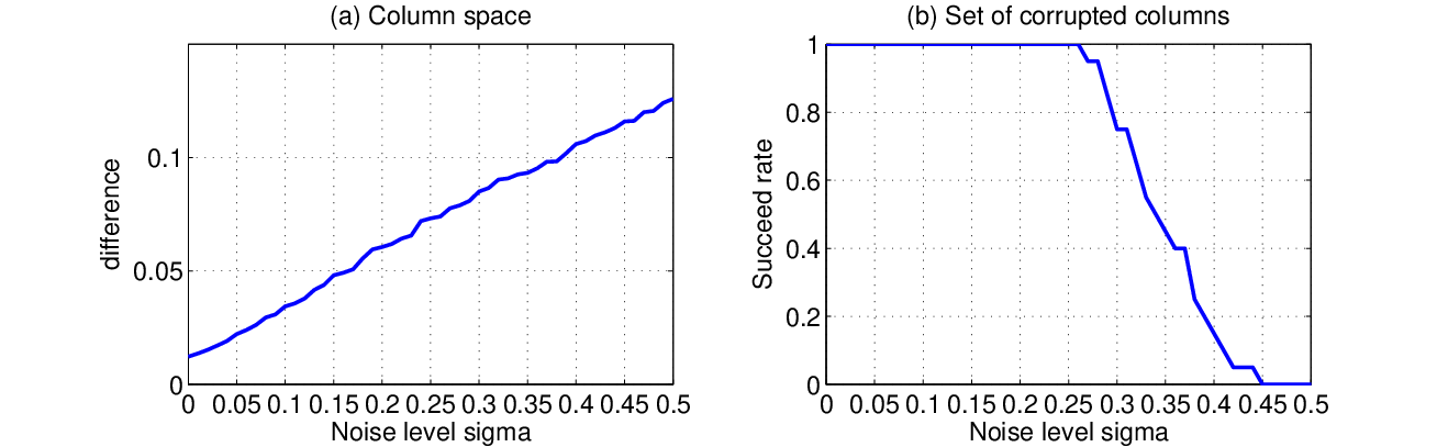
Fig. 9: Performance of Method 1 for different noise level σ\sigma

Fig. 9 shows the difference between the original and reconstructed column space (‖U∗​U∗⁣†−U¯​U¯†‖\|U^{*}U^{*\dagger}-\bar{U}\bar{U}^{\dagger}\|) and the succeed rate for determining the set of corrupted columns according to different noise level σ\sigma. We can see that Method 1 can successfully identify the corrupted columns when the noise level σ\sigma is below 0.25. Method 1 can recover the column space with small errors when σ\sigma is smaller than 0.1.

V-B Comparison with other methods on synthetic data

V-B1 D¯=C¯​WT\bar{D}=\bar{C}W^{T} is column-sparse

Refs. [34] [22] considered matrix decomposition problem when D¯\bar{D} is column-sparse and scattered-sparse, respectively. We compare our method with them in the special case that D¯=C¯​WT\bar{D}=\bar{C}W^{T} is column-sparse. Fix t=p=50t=p=50, n=20n=20, and r=2r=2. We generate L¯\bar{L} and C¯\bar{C} with the same rules as in Section V-A. We generate a binary matrix WW ∈\in ℝp×n\mathbb{R}^{p\times n} with two ‘1’s each row and five ‘1’s each column. Then the ratio of support sizes of D¯\bar{D} and C¯\bar{C} is about five. D¯\bar{D} is column-sparse when C¯\bar{C} is column-sparse. We simulate the measurement matrix MM according to (8) with N=0N=0. λ\lambda in our method is set to be 0.9. λ\lambda’s in methods of [34] and [22] are set to be 0.5 and 0.1, respectively.

Refer to caption
Fig. 10: Success rates when D¯=C¯​WT\bar{D}=\bar{C}W^{T} is column-sparse.

Fig. 10 shows the success rates of three methods with different support sizes of C¯\bar{C}. Our method performs the best since we exploit the structure D¯=C¯​WT\bar{D}=\bar{C}W^{T} besides sparsity. The false alarm rate of our method is zero.

V-B2 Combination of attack patterns.

We consider the general case that the attacks satisfy (14). We use the generalized version in (15)-(16) to detect combined attacks. λ1\lambda_{1} and λ2\lambda_{2} in (15) are set to be 1 and 0.1, respectively. λ\lambda’s in methods of [34] and [22] are set to be 0.5 and 0.1, respectively. L¯\bar{L}, C¯\bar{C}, and WW are generated the same as above. S¯\bar{S} is a sparse matrix with nonzero entries independently drawn from 𝒩⁡(0,1)\mathcal{N}(0,1). We define the correct estimation of the column space of L¯\bar{L} as a successful recovery. Fig. 11 compares the methods when C¯\bar{C} is a zero matrix. The attacks are scattered-sparse, and our method performs as well as that in [22]. Fig. 12 compares the methods when both column-sparse and scattered-sparse attacks exist. Besides a sparse S¯\bar{S}, we randomly select two columns in C¯\bar{C} and select their entries independently from 𝒩⁡(0,1)\mathcal{N}(0,1). Only our method succeeds when both attacks exist.

Refer to caption
Fig. 11: Success rates when D¯=S¯\bar{D}=\bar{S} is scattered-sparse.
Refer to caption
Fig. 12: Success rates when D¯=C¯​WT+S¯\bar{D}=\bar{C}W^{T}+\bar{S}.

V-C Performance comparison on actual PMU data

We consider the PMU data shown in Section II-A. Two two-second PMU datasets are tested. One contains ambient data, and the other contains an abnormal event (t=17−19​st=17-19s and t=2−4​st=2-4s in Fig. 2, respectively). We first inject data attacks as an intruder and then use Method 1 to detect the attacks.

We consider the scenario that an intruder alters the PMU channels that measure I12I^{12},I52I^{52},I13I^{13} and I43I^{43} in order to corrupt voltage estimations of Buses 2 and 3. Fig. 13 visualizes the actual PMU data and the data after the injection of attacks for two 2-second datasets. η\eta and λ\lambda are set to be 5 and 1 respectively in Method 1. Fig. 14 shows the ℓ2\ell_{2} norm of each column of the resulting D¯\bar{D} matrix. The columns with significant ℓ2\ell_{2} norm correspond to channels that measure I12I^{12},I52I^{52},I13I^{13} and I43I^{43}. Therefore, our method successfully identifies the four PMU channels under attack. We repeat the same experiment when an intruder alters the channels that measure V5V^{5}, I52I^{52}, I54I^{54}, I59I^{59}, and I45I^{45} to corrupt voltage estimation of Buses 5. Fig. 15 shows the ℓ2\ell_{2} norm of each column of the resulting C¯\bar{C} matrix in this case. The column with significant ℓ2\ell_{2} norm corresponds Bus 5. Thus the recovery is also successful.

Refer to caption
Fig. 13: The actual PMU data and PMU data under attack
Refer to caption
Fig. 14: ℓ2\ell_{2} norm of each column of D¯\bar{D}
Refer to caption
Fig. 15: ℓ2\ell_{2} norm of each column of C¯\bar{C}

Fig. 16 compares our method and that in [34] on the ambient PMU data. Given support size of C¯\bar{C}, the result is averaged over all possible attack locations. Our method outperforms [34] because we exploit (7) to reduce the degree of freedom in D¯\bar{D}. For example, 7 out of 23 channels needs to be attacked to change the state of Bus 1. That means 30% of the columns of D¯\bar{D} are nonzero. This high percentage of corruption in D¯\bar{D} cannot be handedly by [34].

Refer to caption
Fig. 16: Success rates with varying support size of C¯\bar{C}, or equivalently, the number of affected system states.

VI Conclusion

We address the problem of detecting successive unobservable cyber data attacks to PMU measurements. We formulate the identification problem as a matrix decomposition problem of a low-rank matrix and a transformed column-sparse matrix. We propose a convex-optimization-based method and provide its theoretical guarantee. Although motivated by power system monitoring, our results on matrix decomposition can be applied to other scenarios. One future direction is the analysis of the detection performance when some of the measurements are lost during the communication to the central operator.

Acknowledgement

We thank New York Power Authority for providing PMU data for the Central NY Power System. This research is supported in part by the ERC Program of NSF and DoE under the supplement to NSF Award EEC-1041877 and the CURENT Industry Partnership Program, and in part by NSF Grant 1508875, NYSERDA Grants #36653 and #28815.

References

  • [1] A. Abur and A. G. Exposito, Power system state estimation: theory and implementation. CRC Press, 2004.
  • [2] R. Basri and D. W. Jacobs, “Lambertian reflectance and linear subspaces,” IEEE Trans. Pattern Anal. Mach. Intell., vol. 25, no. 2, pp. 218–233, 2003.
  • [3] R. B. Bobba, K. M. Rogers, Q. Wang, H. Khurana, K. Nahrstedt, and T. J. Overbye, “Detecting false data injection attacks on DC state estimation,” in Proc. the First Workshop on Secure Control Systems (SCS), 2010.
  • [4] E. J. Candès, X. Li, Y. Ma, and J. Wright, “Robust principal component analysis?” Journal of the ACM (JACM), vol. 58, no. 3, p. 11, 2011.
  • [5] V. Chandrasekaran, S. Sanghavi, P. A. Parrilo, and A. S. Willsky, “Rank-sparsity incoherence for matrix decomposition,” SIAM Journal on Optimization, vol. 21, no. 2, pp. 572–596, 2011.
  • [6] J. Chen and A. Abur, “Placement of PMUs to enable bad data detection in state estimation,” IEEE Trans. Power Syst., vol. 21, no. 4, pp. 1608–1615, 2006.
  • [7] Y. Chen, L. Xie, and P. Kumar, “Dimensionality reduction and early event detection using online synchrophasor data,” in Proc. IEEE Power and Energy Society General Meeting, 2013, pp. 1–5.
  • [8] N. Dahal, R. L. King, and V. Madani, “Online dimension reduction of synchrophasor data,” in Proc. IEEE PES Transmission and Distribution Conference and Exposition (T&D), 2012, pp. 1–7.
  • [9] G. Dán and H. Sandberg, “Stealth attacks and protection schemes for state estimators in power systems,” in Proc. IEEE International Conference on Smart Grid Communications (SmartGridComm), 2010, pp. 214–219.
  • [10] J. P. Finn, K. Nael, V. Deshpande, O. Ratib, and G. Laub, “Cardiac MR imaging: State of the technology1,” Radiology, vol. 241, no. 2, pp. 338–354, 2006.
  • [11] H. Gao, J.-F. Cai, Z. Shen, and H. Zhao, “Robust principal component analysis-based four-dimensional computed tomography,” Physics in medicine and biology, vol. 56, no. 11, p. 3181, 2011.
  • [12] P. Gao, M. Wang, S. Ghiocel, and J. H. Chow, “Modeless reconstruction of missing synchrophasor measurements,” in Proc. IEEE PES General Meeting (selected in Best Papers Sessions), 2014.
  • [13] M. Grant and S. Boyd, “CVX: Matlab software for disciplined convex programming, version 1.21,” http://cvxr.com/, Oct. 2010.
  • [14] E. Handschin, F. Schweppe, J. Kohlas, and A. Fiechter, “Bad data analysis for power system state estimation,” IEEE Trans. Power App. Syst., vol. 94, no. 2, pp. 329–337, 1975.
  • [15] C. Herridge, M. Levine, M. Emanuel, and M. Oinounou, “Sources: Staged cyber attack reveals vulnerability in power grid,” http://www.foxnews.com/politics/2009/04/08/cyberspies-penetrate-power-grid-leave-software-disrupt/, 2009.
  • [16] R. A. Horn and C. R. Johnson, Matrix analysis. Cambridge university press, 2012.
  • [17] T. Kim and H. Poor, “Strategic protection against data injection attacks on power grids,” IEEE Trans. Smart Grid, vol. 2, no. 2, pp. 326–333, 2011.
  • [18] O. Kosut, L. Jia, R. Thomas, and L. Tong, “Malicious data attacks on smart grid state estimation: Attack strategies and countermeasures,” in Proc. IEEE International Conference on Smart Grid Communications (SmartGridComm), 2010, pp. 220–225.
  • [19] A. Lakhina, M. Crovella, and C. Diot, “Diagnosing network-wide traffic anomalies,” in ACM SIGCOMM Computer Communication Review, vol. 34, no. 4, 2004, pp. 219–230.
  • [20] Y. Li and D. Wang, “Separation of singing voice from music accompaniment for monaural recordings,” IEEE Trans. Audio, Speech, Language Process., vol. 15, no. 4, pp. 1475–1487, 2007.
  • [21] Z. Lin, A. Ganesh, J. Wright, L. Wu, M. Chen, and Y. Ma, “Fast convex optimization algorithms for exact recovery of a corrupted low-rank matrix,” Computational Advances in Multi-Sensor Adaptive Processing (CAMSAP), vol. 61, 2009.
  • [22] L. Liu, M. Esmalifalak, Q. Ding, V. A. Emesih, and Z. Han, “Detecting false data injection attacks on power grid by sparse optimization,” IEEE Trans. Smart Grid, vol. 5, no. 2, pp. 612–621, 2014.
  • [23] Y. Liu, P. Ning, and M. K. Reiter, “False data injection attacks against state estimation in electric power grids,” ACM Transactions on Information and System Security (TISSEC), vol. 14, no. 1, p. 13, 2011.
  • [24] M. Mardani, G. Mateos, and G. Giannakis, “Recovery of low-rank plus compressed sparse matrices with application to unveiling traffic anomalies,” IEEE Trans. Inf. Theory, vol. 59, no. 8, pp. 5186–5205, 2013.
  • [25] H. M. Merrill and F. C. Schweppe, “Bad data suppression in power system static state estimation,” IEEE Trans. Power App. Syst., no. 6, pp. 2718–2725, 1971.
  • [26] J. Meserve, “Sources: Staged cyber attack reveals vulnerability in power grid,” http://www.cnn.com/2007/US/09/26/power.at.risk/, 2007.
  • [27] A. Monticelli and A. Garcia, “Reliable bad data processing for real-time state estimation,” IEEE Trans. Power App. Syst., no. 5, pp. 1126–1139, 1983.
  • [28] B. Recht, M. Fazel, and P. A. Parrilo, “Guaranteed minimum-rank solutions of linear matrix equations via nuclear norm minimization,” SIAM Rev., vol. 52, no. 3, pp. 471–501, 2010.
  • [29] H. Sandberg, A. Teixeira, and K. H. Johansson, “On security indices for state estimators in power networks,” in Proc. the First Workshop on Secure Control Systems (SCS), 2010.
  • [30] H. Sedghi and E. Jonckheere, “Statistical structure learning of smart grid for detection of false data injection,” in Proc. IEEE Power and Energy Society General Meeting (PES), 2013, pp. 1–5.
  • [31] A. Tajer, S. Kar, H. V. Poor, and S. Cui, “Distributed joint cyber attack detection and state recovery in smart grids,” in Proc. IEEE International Conference on Smart Grid Communications (SmartGridComm), 2011, pp. 202–207.
  • [32] M. Thottan and C. Ji, “Anomaly detection in IP networks,” IEEE Trans. Signal Process., vol. 51, no. 8, pp. 2191–2204, 2003.
  • [33] M. Wang, P. Gao, S. Ghiocel, J. H. Chow, B. Fardanesh, G. Stefopoulos, and M. P. Razanousky, “Identification of "unobservable" cyber data attacks on power grids,” in Proc. IEEE SmartGridComm, 2014.
  • [34] H. Xu, C. Caramanis, and S. Sanghavi, “Robust pca via outlier pursuit,” IEEE Trans. Inf. Theory, vol. 58, no. 5, pp. 3047–3064, May 2012.
  • [35] W. Xu, M. Wang, L. Lai, and A. Tang, “Sparse error correction from nonlinear measurements with applications in bad data detection for power networks,” IEEE Trans. Signal Process., vol. 61, no. 24, pp. 6175–6187, 2013.

Appendix

VI-A Proof of Lemma 1

Proof:

We first state the following result that will be used in the proof.

Lemma 7 (Geršhgorin circle theorem [16]).

Let A be a complex n×nn\times n matrix, with entries ai​ja_{ij}. Then, every eigenvalue of A lies within at least one of the Geršhgorin discs Di​(A)​(i=1,…,n)D_{i}(A)(i=1,...,n), where Di​(A):={z∈ℂ:|z−ai​i|≤∑j≠i|ai​j|}D_{i}(A):=\{z\in\mathbb{C}:|z-a_{ii}|\leq\sum_{j\neq{i}}\left|a_{ij}\right|\}.

For any given ℐ{\mathcal{I}} with |ℐ|≤k|{\mathcal{I}}|\leq k, since WW has unit-norm columns, and |Wi†​Wj|≤μ|W^{\dagger}_{i}W_{j}|\leq\mu for all i≠ji\neq j, from Geršhgorin circle theorem, we have ‖I−Wℐ†​Wℐ‖≤(k−1)​μ<1\|I-W^{\dagger}_{{\mathcal{I}}}W_{{\mathcal{I}}}\|\leq(k-1)\mu<1, where the last inequality follows from k​μ<1k\mu<1. Then,

‖(Wℐ†​Wℐ)−1‖=\displaystyle\|(W^{\dagger}_{{\mathcal{I}}}W_{{\mathcal{I}}})^{-1}\|= ‖∑i=0∞(I−Wℐ†​Wℐ)i‖≤∑i=0∞‖(I−Wℐ†​Wℐ)i‖\displaystyle\|\sum_{i=0}^{\infty}(I-W^{\dagger}_{{\mathcal{I}}}W_{{\mathcal{I}}})^{i}\|\leq\sum_{i=0}^{\infty}\|(I-W^{\dagger}_{{\mathcal{I}}}W_{{\mathcal{I}}})^{i}\|
≤\displaystyle\leq 1/(1−(k−1)​μ).\displaystyle 1/(1-(k-1)\mu).

The lemma follows from the definition of σk\sigma_{k}. ∎

VI-B Proof of Lemma 3

Proof:

For any Δ∈ℂt×n\Delta\in\mathbb{C}^{t\times n}, ⟨L′+Δ​WT,C′−Δ⟩\langle L^{\prime}+\Delta W^{T},C^{\prime}-\Delta\rangle is feasible to (13). Let GG be such that ‖G‖=1\|G\|=1, ⟨G,𝒫T′⁣⟂​(Δ​WT)⟩=‖𝒫T′⁣⟂​(Δ​WT)‖∗\left\langle G,{\mathcal{P}}_{T^{\prime\perp}}(\Delta W^{T})\right\rangle=\|{\mathcal{P}}_{T^{\prime\perp}}(\Delta W^{T})\|_{*} and 𝒫T′​(G)=0{\mathcal{P}}_{T^{\prime}}(G)=0. Then 𝒫T′​(Q)+G{\mathcal{P}}_{T^{\prime}}(Q)+G is a subgradient of ‖L′‖∗\|L^{\prime}\|_{*}. Let FF be such that Fi=−Δi/∥Δi∥2F_{i}=-\Delta_{i}/\|\Delta_{i}\|_{2} if i∈ℐ¯ci\in\bar{{\mathcal{I}}}^{c} and Δi≠𝟎\Delta_{i}\neq\bm{0}, and Fi=𝟎F_{i}=\bm{0} otherwise. Then 𝒫ℐ¯​(Q​W‡)/λ+F{\mathcal{P}}_{\bar{{\mathcal{I}}}}(QW^{\ddagger})/\lambda+F is a subgradient of ‖C′‖1,2\|C^{\prime}\|_{1,2}. Then

‖L′+Δ​WT‖∗+λ​‖C′−Δ‖1,2−‖L′‖∗−λ​‖C′‖1,2\displaystyle\|L^{\prime}+\Delta W^{T}\|_{*}+\lambda\|C^{\prime}-\Delta\|_{1,2}-\|L^{\prime}\|_{*}-\lambda\|C^{\prime}\|_{1,2} (43)
≥\displaystyle\geq ⟨𝒫T′​(Q)+G,Δ​WT⟩−λ⁡⟨𝒫ℐ¯​(Q​W‡)/λ+F,Δ⟩\displaystyle\langle{\mathcal{P}}_{T^{\prime}}(Q)+G,\Delta W^{T}\rangle-\lambda\langle{\mathcal{P}}_{\bar{{\mathcal{I}}}}(QW^{\ddagger})/\lambda+F,\Delta\rangle
=\displaystyle= ‖𝒫T′⁣⟂​(Δ​WT)‖∗+λ​‖𝒫ℐ¯c​(Δ)‖1,2+⟨Q−𝒫T′⁣⟂​(Q),Δ​WT⟩\displaystyle\|{\mathcal{P}}_{T^{\prime\perp}}(\Delta W^{T})\|_{*}+\lambda\|{\mathcal{P}}_{\bar{{\mathcal{I}}}^{c}}(\Delta)\|_{1,2}+\langle Q-{\mathcal{P}}_{T^{\prime\perp}}(Q),\Delta W^{T}\rangle
−⟨Q​W‡−𝒫ℐ¯c​(Q​W‡),Δ⟩\displaystyle-\langle QW^{\ddagger}-{\mathcal{P}}_{\bar{{\mathcal{I}}}^{c}}(QW^{\ddagger}),\Delta\rangle
≥\displaystyle\geq (1−‖𝒫T′⁣⟂​(Q)‖)​‖𝒫T′⁣⟂​(Δ​WT)‖∗\displaystyle(1-\|{\mathcal{P}}_{T^{\prime\perp}}(Q)\|)\|{\mathcal{P}}_{T^{\prime\perp}}(\Delta W^{T})\|_{*}
+(λ−‖(Q​W‡)ℐ¯c‖∞,2)​‖𝒫ℐ¯c​(Δ)‖1,2\displaystyle+(\lambda-\|(QW^{\ddagger})_{\bar{{\mathcal{I}}}^{c}}\|_{\infty,2})\|{\mathcal{P}}_{\bar{{\mathcal{I}}}^{c}}(\Delta)\|_{1,2}
≥\displaystyle\geq 0\displaystyle 0

From (43), ⟨L′,C′⟩\langle L^{\prime},C^{\prime}\rangle is an optimal solution to (13). If (34) holds with strict inequality, the last inequality of (43) is strict unless

‖𝒫T′⁣⟂​(Δ​WT)‖∗=‖𝒫ℐ¯c​(Δ)‖1,2=0.\|{\mathcal{P}}_{T^{\prime\perp}}(\Delta W^{T})\|_{*}=\|{\mathcal{P}}_{\bar{{\mathcal{I}}}^{c}}(\Delta)\|_{1,2}=0. (44)

(44) implies that Δ​WT∈𝒫T′\Delta W^{T}\in{\mathcal{P}}_{T^{\prime}} and Δ∈𝒫ℐ¯\Delta\in{\mathcal{P}}_{\bar{{\mathcal{I}}}}. Note that Δ∈𝒫ℐ¯\Delta\in{\mathcal{P}}_{\bar{{\mathcal{I}}}} implies that Δ​WT∈𝒫𝒥¯\Delta W^{T}\in{\mathcal{P}}_{\bar{{\mathcal{J}}}}. Then

𝒫𝒥¯​(Δ​WT)\displaystyle{\mathcal{P}}_{\bar{{\mathcal{J}}}}(\Delta W^{T}) =Δ​WT=𝒫T′​(Δ​WT)\displaystyle=\Delta W^{T}={\mathcal{P}}_{T^{\prime}}(\Delta W^{T})
=𝒫U′​(Δ​WT)+𝒫V′​𝒫U′⁣⟂​(Δ​WT)\displaystyle={\mathcal{P}}_{U^{\prime}}(\Delta W^{T})+{\mathcal{P}}_{V^{\prime}}{\mathcal{P}}_{U^{\prime\perp}}(\Delta W^{T})
=𝒫𝒥¯​𝒫U′​(Δ​WT)+𝒫V′​𝒫U′⁣⟂​(Δ​WT),\displaystyle={\mathcal{P}}_{\bar{{\mathcal{J}}}}{\mathcal{P}}_{U^{\prime}}(\Delta W^{T})+{\mathcal{P}}_{V^{\prime}}{\mathcal{P}}_{U^{\prime\perp}}(\Delta W^{T}), (45)

where the last equality holds since 𝒫𝒥¯​(Δ​WT)=Δ​WT{\mathcal{P}}_{\bar{{\mathcal{J}}}}(\Delta W^{T})=\Delta W^{T}. Thus, from (45) we have 𝒫𝒥¯​𝒫U′⁣⟂​(Δ​WT)=𝒫V′​𝒫U′⁣⟂​(Δ​WT){\mathcal{P}}_{\bar{{\mathcal{J}}}}{\mathcal{P}}_{U^{\prime\perp}}(\Delta W^{T})={\mathcal{P}}_{V^{\prime}}{\mathcal{P}}_{U^{\prime\perp}}(\Delta W^{T}), which means 𝒫U′⁣⟂​(Δ​WT)∈𝒫𝒥¯∩𝒫V′{\mathcal{P}}_{U^{\prime\perp}}(\Delta W^{T})\in{\mathcal{P}}_{\bar{{\mathcal{J}}}}\cap{\mathcal{P}}_{V^{\prime}}. Then 𝒫U′⁣⟂​(Δ​WT){\mathcal{P}}_{U^{\prime\perp}}(\Delta W^{T}) is 00 from the assumption. Then, 𝒫U¯​(Δ​WT)=𝒫U′​(Δ​WT)=Δ​WT{\mathcal{P}}_{\bar{U}}(\Delta W^{T})={\mathcal{P}}_{U^{\prime}}(\Delta W^{T})=\Delta W^{T}, where the first equality holds from (33). Therefore, for any optimal solution ⟨L′+Δ​WT,C′−Δ⟩\langle L^{\prime}+\Delta W^{T},C^{\prime}-\Delta\rangle for some Δ≠0\Delta\neq 0 to (13), Δ​WT∈𝒫U¯\Delta W^{T}\in{\mathcal{P}}_{\bar{U}}, and Δ∈𝒫ℐ¯\Delta\in{\mathcal{P}}_{\bar{{\mathcal{I}}}}. The claim follows. ∎

VI-C Construction of QQ

Here we demonstrate that QQ in (39) is well defined. The key is to show (a) there exists H^∈𝔊⁡(C′)\hat{H}\in{\mathfrak{G}}(C^{\prime}) such that (35) holds, and (b) the infinite sum in (37) converges. We prove these two properties through the following lemmas.

Lemma 8.

There exists H^∈𝔊⁡(C′)\hat{H}\in{\mathfrak{G}}(C^{\prime}) such that (35) holds.

Proof.

Since ⟨L′,C′⟩\langle L^{\prime},C^{\prime}\rangle is an optimal solution to the Oracle problem (32), there exists G′,A′∈ℂt×pG^{\prime},A^{\prime}\in\mathbb{C}^{t\times p}, B′,Z∈ℂt×nB^{\prime},Z\in\mathbb{C}^{t\times n}, and some H^∈𝔊⁡(C)\hat{H}\in{\mathfrak{G}}(C) such that

(U¯​V^†+G′+𝒫U¯⟂​(A′))​W‡=λ⁡(H^+Z)+𝒫ℐc​(B′),(\bar{U}\hat{V}^{\dagger}+G^{\prime}+{\mathcal{P}}_{\bar{U}^{\perp}}(A^{\prime}))W^{\ddagger}=\lambda(\hat{H}+Z)+{\mathcal{P}}_{{\mathcal{I}}^{c}}(B^{\prime}), (46)

where 𝒫T′⁣⟂​(G′)=0{\mathcal{P}}_{T^{\prime\perp}}(G^{\prime})=0 and 𝒫ℐ​(Z)=0{\mathcal{P}}_{{\mathcal{I}}}(Z)=0. Then

𝒫U¯​𝒫ℐ¯​(((U¯​V^†+G′+𝒫U¯⟂​(A′))​W‡)=U¯​V^†​Wℐ¯‡CLOSE,{\mathcal{P}}_{\bar{U}}{\mathcal{P}}_{\bar{{\mathcal{I}}}}(((\bar{U}\hat{V}^{\dagger}+G^{\prime}+{\mathcal{P}}_{\bar{U}^{\perp}}(A^{\prime}))W^{\ddagger})=\bar{U}\hat{V}^{\dagger}W^{\ddagger}_{\bar{{\mathcal{I}}}}, (47)
𝒫U¯​𝒫ℐ¯​(λ⁡(H^+Z)+𝒫ℐc​(B′))=λ​𝒫U¯​𝒫ℐ¯​(H^)=λ​U¯​U¯†​H^{\mathcal{P}}_{\bar{U}}{\mathcal{P}}_{\bar{{\mathcal{I}}}}(\lambda(\hat{H}+Z)+{\mathcal{P}}_{{\mathcal{I}}^{c}}(B^{\prime}))=\lambda{\mathcal{P}}_{\bar{U}}{\mathcal{P}}_{\bar{{\mathcal{I}}}}(\hat{H})=\lambda\bar{U}\bar{U}^{\dagger}\hat{H} (48)

Combining (46)-(48), we have

U¯​V^†​Wℐ¯‡=λ​U¯​U¯†​H^.\bar{U}\hat{V}^{\dagger}W^{\ddagger}_{\bar{{\mathcal{I}}}}=\lambda\bar{U}\bar{U}^{\dagger}\hat{H}. (49)

By multiplying U¯†\bar{U}^{\dagger} to both sides of (49), we obtain Lemma 8. ∎

Lemma 9.
ψ:=‖𝒫V^​𝒫Wℐ¯​𝒫V^‖≤ψ~<1\psi:=\|{\mathcal{P}}_{\hat{V}}{\mathcal{P}}_{W_{\bar{{\mathcal{I}}}}}{\mathcal{P}}_{\hat{V}}\|\leq\tilde{\psi}<1
Proof.
‖𝒫V^​𝒫Wℐ¯​𝒫V^​(X)‖\displaystyle\|{\mathcal{P}}_{\hat{V}}{\mathcal{P}}_{W_{\bar{{\mathcal{I}}}}}{\mathcal{P}}_{\hat{V}}(X)\|
=\displaystyle= ‖X​V^​V^†​Wℐ¯‡​(Wℐ¯T​Wℐ¯‡)−1​Wℐ¯T​V^​V^†‖\displaystyle\|X\hat{V}\hat{V}^{\dagger}W^{\ddagger}_{\bar{{\mathcal{I}}}}(W_{\bar{{\mathcal{I}}}}^{T}W^{\ddagger}_{\bar{{\mathcal{I}}}})^{-1}W_{\bar{{\mathcal{I}}}}^{T}\hat{V}\hat{V}^{\dagger}\|
=(a)\displaystyle\stackrel{{\scriptstyle(\rm{a})}}{{=}} ‖X​V^​(λ​U¯†​H^)​(Wℐ¯T​Wℐ¯‡)−1​(λ​U¯†​H^)†​V^†‖\displaystyle\|X\hat{V}(\lambda\bar{U}^{\dagger}\hat{H})(W_{\bar{{\mathcal{I}}}}^{T}W^{\ddagger}_{\bar{{\mathcal{I}}}})^{-1}(\lambda\bar{U}^{\dagger}\hat{H})^{\dagger}\hat{V}^{\dagger}\|
≤\displaystyle\leq ‖X‖​‖V^​U¯†‖​‖λ​H^​‖‖(Wℐ¯†​Wℐ¯)−1‖​‖λ​H^†‖‖​U¯​V^†‖\displaystyle\|X\|\|\hat{V}\bar{U}^{\dagger}\|\|\lambda\hat{H}\|\|(W_{\bar{{\mathcal{I}}}}^{\dagger}W_{\bar{{\mathcal{I}}}})^{-1}\|\|\lambda\hat{H}^{\dagger}\|\|\bar{U}\hat{V}^{\dagger}\|
≤(b)\displaystyle\stackrel{{\scriptstyle(\rm{b})}}{{\leq}} ‖X‖⋅1⋅λ​k⋅σk⋅λ​k⋅1\displaystyle\|X\|\cdot 1\cdot\lambda\sqrt{k}\cdot\sigma_{k}\cdot\lambda\sqrt{k}\cdot 1
≤(c)\displaystyle\stackrel{{\scriptstyle(\rm{c})}}{{\leq}} ‖X‖​λmax​k~​σk~=(d)‖X‖​ψ~,\displaystyle\|X\|\lambda_{\max}\tilde{k}\sigma_{\tilde{k}}\stackrel{{\scriptstyle(\rm{d})}}{{=}}\|X\|\tilde{\psi},

where (a) follows from Lemma 8, (b) follows from the fact that H^\hat{H} has at most kk nonzero columns with unit-norm, (c) follows from the property that λ≤λmax\lambda\leq\lambda_{\max}, k≤k~k\leq\tilde{k} and σk≤σk~\sigma_{k}\leq\sigma_{\tilde{k}}, and (d) follows from the definition of ψ~\tilde{\psi}. Then Lemma 9 follows. ∎

Lemma 10.

𝒫V^​(I−𝒫Wℐ¯)​𝒫V^{\mathcal{P}}_{\hat{V}}(I-{\mathcal{P}}_{W_{\bar{{\mathcal{I}}}}}){\mathcal{P}}_{\hat{V}} is an injection from 𝒫V^{\mathcal{P}}_{\hat{V}} to 𝒫V^{\mathcal{P}}_{\hat{V}}, and its inverse operation is (I+∑i=1∞(𝒫V^​𝒫Wℐ¯​𝒫V^)i)(I+\sum_{i=1}^{\infty}({\mathcal{P}}_{\hat{V}}{\mathcal{P}}_{W_{\bar{{\mathcal{I}}}}}{\mathcal{P}}_{\hat{V}})^{i}).

Proof.

Since ‖𝒫V^​𝒫Wℐ¯​𝒫V^‖<1\|{\mathcal{P}}_{\hat{V}}{\mathcal{P}}_{W_{\bar{{\mathcal{I}}}}}{\mathcal{P}}_{\hat{V}}\|<1 from Lemma 9, then (I+∑i=1∞(𝒫V^​𝒫Wℐ¯​𝒫V^)i)(I+\sum_{i=1}^{\infty}({\mathcal{P}}_{\hat{V}}{\mathcal{P}}_{W_{\bar{{\mathcal{I}}}}}{\mathcal{P}}_{\hat{V}})^{i}) is well defined. For any X∈𝒫V^X\in{\mathcal{P}}_{\hat{V}}, we have

𝒫V^​(I−𝒫Wℐ¯)​𝒫V^​(I+∑i=1∞(𝒫V^​𝒫Wℐ¯​𝒫V^)i)​(X)\displaystyle{\mathcal{P}}_{\hat{V}}(I-{\mathcal{P}}_{W_{\bar{{\mathcal{I}}}}}){\mathcal{P}}_{\hat{V}}(I+\sum_{i=1}^{\infty}({\mathcal{P}}_{\hat{V}}{\mathcal{P}}_{W_{\bar{{\mathcal{I}}}}}{\mathcal{P}}_{\hat{V}})^{i})(X)
=\displaystyle= 𝒫V^​(I−𝒫V^​𝒫Wℐ¯​𝒫V^)​(I+∑i=1∞(𝒫V^​𝒫Wℐ¯​𝒫V^)i)​(X)\displaystyle{\mathcal{P}}_{\hat{V}}(I-{\mathcal{P}}_{\hat{V}}{\mathcal{P}}_{W_{\bar{{\mathcal{I}}}}}{\mathcal{P}}_{\hat{V}})(I+\sum_{i=1}^{\infty}({\mathcal{P}}_{\hat{V}}{\mathcal{P}}_{W_{\bar{{\mathcal{I}}}}}{\mathcal{P}}_{\hat{V}})^{i})(X)
=\displaystyle= 𝒫V^​(X)=X.\displaystyle{\mathcal{P}}_{\hat{V}}(X)=X. (50)

Then the lemma follows. ∎

VI-D Proof of Lemma 4

Proof.

We need to show that QQ defined in (39) satisfies all the conditions in (34). We first summarize some properties that will be used in the proof. Since WW has unit-norm columns, |Wi†​Wj|≤μ|W^{\dagger}_{i}W_{j}|\leq\mu for all i≠ji\neq j, and |ℐ¯|≤k|\bar{{\mathcal{I}}}|\leq k, we have

‖Wℐ¯‖=λmax​(Wℐ¯†​Wℐ¯)≤1+(k−1)​μ,\|W_{\bar{{\mathcal{I}}}}\|=\sqrt{\lambda_{\max}(W_{\bar{{\mathcal{I}}}}^{\dagger}W_{\bar{{\mathcal{I}}}})}\leq\sqrt{1+(k-1)\mu}, (51)

where the inequality follows from the Geršhgorin circle theorem. From |ℐ¯|≤k|\bar{{\mathcal{I}}}|\leq k and |Wi†​Wj|≤μ|W^{\dagger}_{i}W_{j}|\leq\mu for all i≠ji\neq j, we have ‖(Wℐ¯†​Wℐ¯c)‖∞,2≤k​μ\|(W_{\bar{{\mathcal{I}}}}^{\dagger}W_{\bar{{\mathcal{I}}}^{c}})\|_{\infty,2}\leq\sqrt{k}\mu. Since H^\hat{H} has at most kk unit-norm columns while other columns are zero, we have

‖λ​H^‖≤λ​k.\|\lambda\hat{H}\|\leq\lambda\sqrt{k}. (52)

Step 1: verification of (a) of (34).

𝒫U′​(Q)=(a)𝒫U¯​(Q)=U¯​V^†+𝒫U¯​(Φ)−𝒫U¯​(Φ)−0=U¯​V^†,{\mathcal{P}}_{U^{\prime}}(Q)\stackrel{{\scriptstyle(\rm{a})}}{{=}}{\mathcal{P}}_{\bar{U}}(Q)=\bar{U}\hat{V}^{\dagger}+{\mathcal{P}}_{\bar{U}}(\Phi)-{\mathcal{P}}_{\bar{U}}(\Phi)-0=\bar{U}\hat{V}^{\dagger}, (53)

where (a) follows from (23). From (33), we have

V^​V^†=V′​U′⁣†​U¯​U¯†​U′​V′⁣†=(b)V′​U′⁣†​U′​U′⁣†​U′​V′⁣†=V′​V′⁣†,\hat{V}\hat{V}^{\dagger}=V^{\prime}U^{\prime{\dagger}}\bar{U}\bar{U}^{\dagger}U^{\prime}V^{\prime\dagger}\stackrel{{\scriptstyle(\rm{b})}}{{=}}V^{\prime}U^{\prime{\dagger}}U^{\prime}U^{\prime{\dagger}}U^{\prime}V^{\prime\dagger}=V^{\prime}V^{\prime\dagger},

where (b) follows from (33). Thus, 𝒫V′​(⋅)=𝒫V^​(⋅){\mathcal{P}}_{V^{\prime}}(\cdot)={\mathcal{P}}_{\hat{V}}(\cdot). Then

𝒫V′​(Q)\displaystyle{\mathcal{P}}_{V^{\prime}}(Q) =𝒫V^​(Q)=(c)U¯​V^†+𝒫V^​(Φ)−𝒫V^​𝒫U¯​(Φ)\displaystyle={\mathcal{P}}_{\hat{V}}(Q)\stackrel{{\scriptstyle(\rm{c})}}{{=}}\bar{U}\hat{V}^{\dagger}+{\mathcal{P}}_{\hat{V}}(\Phi)-{\mathcal{P}}_{\hat{V}}{\mathcal{P}}_{\bar{U}}(\Phi)
−𝒫V^​(I−𝒫Wℐ¯)​𝒫V^​(I+∑i=1∞(𝒫V^​𝒫Wℐ¯CLOSECLOSE\displaystyle-{\mathcal{P}}_{\hat{V}}(I-{\mathcal{P}}_{W_{\bar{{\mathcal{I}}}}}){\mathcal{P}}_{\hat{V}}(I+\sum_{i=1}^{\infty}({\mathcal{P}}_{\hat{V}}{\mathcal{P}}_{W_{\bar{{\mathcal{I}}}}}
OPENOPEN𝒫V^)i)​𝒫V^​𝒫U¯⟂​(Φ)\displaystyle{\mathcal{P}}_{\hat{V}})^{i}){\mathcal{P}}_{\hat{V}}{\mathcal{P}}_{\bar{U}^{\perp}}(\Phi)
=(d)U¯​V^†+𝒫V^​(Φ)−𝒫V^​𝒫U¯​(Φ)−𝒫V^​𝒫U¯⟂​(Φ)\displaystyle\stackrel{{\scriptstyle(\rm{d})}}{{=}}\bar{U}\hat{V}^{\dagger}+{\mathcal{P}}_{\hat{V}}(\Phi)-{\mathcal{P}}_{\hat{V}}{\mathcal{P}}_{\bar{U}}(\Phi)-{\mathcal{P}}_{\hat{V}}{\mathcal{P}}_{\bar{U}^{\perp}}(\Phi)
=U¯​V^†.\displaystyle=\bar{U}\hat{V}^{\dagger}. (54)

(c) follows since 𝒫Wℐ¯{\mathcal{P}}_{W_{\bar{{\mathcal{I}}}}}, 𝒫V^{\mathcal{P}}_{\hat{V}}, and 𝒫V^​𝒫Wℐ¯​𝒫V^{\mathcal{P}}_{\hat{V}}{\mathcal{P}}_{W_{\bar{{\mathcal{I}}}}}{\mathcal{P}}_{\hat{V}} are all given by right matrix multiplication, while 𝒫U¯⟂{\mathcal{P}}_{\bar{U}^{\perp}} is given by left matrix multiplication. (d) follows from Lemma 10. Combining (53) and (54), we obtain that (a) of (34) holds.

Step 2: verification of (b) of (34).

‖𝒫T′⁣⟂​(Q)‖=|𝒫V^⟂​𝒫U¯⟂​(Φ)−\displaystyle\|{\mathcal{P}}_{T^{\prime\perp}}(Q)\|=\|{\mathcal{P}}_{\hat{V}^{\perp}}{\mathcal{P}}_{\bar{U}^{\perp}}(\Phi)-
𝒫U¯⟂𝒫V^⟂(I−𝒫Wℐ¯)𝒫V^(I+∑i=1∞(𝒫V^𝒫Wℐ¯𝒫V^)i)𝒫V^(Φ)∥\displaystyle\quad{\mathcal{P}}_{\bar{U}^{\perp}}{\mathcal{P}}_{\hat{V}^{\perp}}(I-{\mathcal{P}}_{W_{\bar{{\mathcal{I}}}}}){\mathcal{P}}_{\hat{V}}(I+\sum_{i=1}^{\infty}({\mathcal{P}}_{\hat{V}}{\mathcal{P}}_{W_{\bar{{\mathcal{I}}}}}{\mathcal{P}}_{\hat{V}})^{i}){\mathcal{P}}_{\hat{V}}(\Phi)\|
≤\displaystyle\leq ‖Φ‖+(1+∑i=1∞ψi)​‖Φ‖=2−ψ1−ψ​‖Φ‖\displaystyle\|\Phi\|+(1+\sum_{i=1}^{\infty}\psi^{i})\|\Phi\|=\frac{2-\psi}{1-\psi}\|\Phi\|
≤(e)\displaystyle\stackrel{{\scriptstyle(\rm{e})}}{{\leq}} 2−ψ1−ψ​‖λ​H^‖​‖(Wℐ¯†​Wℐ¯)−1‖​‖Wℐ¯T‖\displaystyle\frac{2-\psi}{1-\psi}\|\lambda\hat{H}\|\|(W_{\bar{{\mathcal{I}}}}^{\dagger}W_{\bar{{\mathcal{I}}}})^{-1}\|\|W_{\bar{{\mathcal{I}}}}^{T}\|
≤(f)\displaystyle\stackrel{{\scriptstyle(\rm{f})}}{{\leq}} 2−ψ1−ψ​λ​k​σk​1+(k−1)​μ\displaystyle\frac{2-\psi}{1-\psi}\lambda\sqrt{k}\sigma_{k}\sqrt{1+(k-1)\mu} (55)
≤(g)\displaystyle\stackrel{{\scriptstyle(\rm{g})}}{{\leq}} 2−ψ~1−ψ~​ψ~k~​σk~​k~​σk~​1+(k~−1)​μ\displaystyle\frac{2-\tilde{\psi}}{1-\tilde{\psi}}\sqrt{\frac{\tilde{\psi}}{\tilde{k}\sigma_{\tilde{k}}}}\sqrt{\tilde{k}}\sigma_{\tilde{k}}\sqrt{1+(\tilde{k}-1)\mu} (56)
≤(h)\displaystyle\stackrel{{\scriptstyle(\rm{h})}}{{\leq}} 2−ψ~1−ψ~​ψ~​1+(k~−1)​μ1−(k~−1)​μ\displaystyle\frac{2-\tilde{\psi}}{1-\tilde{\psi}}\sqrt{\tilde{\psi}}\sqrt{\frac{1+(\tilde{k}-1)\mu}{1-(\tilde{k}-1)\mu}} (57)
≤(i)\displaystyle\stackrel{{\scriptstyle(\rm{i})}}{{\leq}} 2−ψ~1−ψ~​ψ~​1+c1−c≤(j)1.\displaystyle\frac{2-\tilde{\psi}}{1-\tilde{\psi}}\sqrt{\tilde{\psi}}\sqrt{\frac{1+c}{1-c}}\stackrel{{\scriptstyle(\rm{j})}}{{\leq}}1.

where (e) follows from the definition of Φ\Phi, and (f) follows from (51) and (52). (g) follows from the property that ψ≤ψ~\psi\leq\tilde{\psi}, 1≤k≤k~1\leq k\leq\tilde{k}, λ≤λmax,k~\lambda\leq\lambda_{\max,\tilde{k}}, and σk≤σk~\sigma_{k}\leq\sigma_{\tilde{k}}. (h) follows from Lemma 1. (i) follow from k~​μ≤c\tilde{k}\mu\leq c, and (j) follows from (19). Then (b) of (34) holds.

Step 3: verification of (c) of (34). First consider

(Δ2​W‡)ℐ¯\displaystyle(\Delta_{2}W^{\ddagger})_{\bar{{\mathcal{I}}}}
=\displaystyle= (𝒫U¯⟂​(I−𝒫Wℐ¯)​𝒫V^​(I+∑i=1∞(𝒫V^​𝒫Wℐ¯​𝒫V^)i)​𝒫V^​(Φ)​W‡)ℐ¯\displaystyle({\mathcal{P}}_{\bar{U}^{\perp}}(I-{\mathcal{P}}_{W_{\bar{{\mathcal{I}}}}}){\mathcal{P}}_{\hat{V}}(I+\sum_{i=1}^{\infty}({\mathcal{P}}_{\hat{V}}{\mathcal{P}}_{W_{\bar{{\mathcal{I}}}}}{\mathcal{P}}_{\hat{V}})^{i}){\mathcal{P}}_{\hat{V}}(\Phi)W^{\ddagger})_{\bar{{\mathcal{I}}}}
=(k)\displaystyle\stackrel{{\scriptstyle(\rm{k})}}{{=}} (𝒫U¯⟂​𝒫V^​(I+∑i=1∞(𝒫V^​𝒫Wℐ¯​𝒫V^)i)​𝒫V^​(Φ))​(I−CLOSE\displaystyle({\mathcal{P}}_{\bar{U}^{\perp}}{\mathcal{P}}_{\hat{V}}(I+\sum_{i=1}^{\infty}({\mathcal{P}}_{\hat{V}}{\mathcal{P}}_{W_{\bar{{\mathcal{I}}}}}{\mathcal{P}}_{\hat{V}})^{i}){\mathcal{P}}_{\hat{V}}(\Phi))(I-
OPENWℐ¯‡​(Wℐ¯T​Wℐ¯‡)−1​Wℐ¯T)​Wℐ¯‡=0\displaystyle W^{\ddagger}_{\bar{{\mathcal{I}}}}(W_{\bar{{\mathcal{I}}}}^{T}W^{\ddagger}_{\bar{{\mathcal{I}}}})^{-1}W_{\bar{{\mathcal{I}}}}^{T})W^{\ddagger}_{\bar{{\mathcal{I}}}}=0

where (k) holds since 𝒫Wℐ¯{\mathcal{P}}_{W_{\bar{{\mathcal{I}}}}}, 𝒫V^{\mathcal{P}}_{\hat{V}}, and 𝒫V^​𝒫Wℐ¯​𝒫V^{\mathcal{P}}_{\hat{V}}{\mathcal{P}}_{W_{\bar{{\mathcal{I}}}}}{\mathcal{P}}_{\hat{V}} are all given by right matrix multiplication, while 𝒫U¯⟂{\mathcal{P}}_{\bar{U}^{\perp}} is given by left matrix multiplication. Then

(Q​W‡)ℐ¯\displaystyle(QW^{\ddagger})_{\bar{{\mathcal{I}}}} =(U¯​V^​W‡+Φ​W‡−𝒫U¯​(Φ)​W‡)ℐ¯−(Δ2​W‡)ℐ¯\displaystyle=(\bar{U}\hat{V}W^{\ddagger}+\Phi W^{\ddagger}-{\mathcal{P}}_{\bar{U}}(\Phi)W^{\ddagger})_{\bar{{\mathcal{I}}}}-(\Delta_{2}W^{\ddagger})_{\bar{{\mathcal{I}}}}
=U¯​V^​Wℐ¯‡+Φ​Wℐ¯‡−𝒫U¯​(Φ)​Wℐ¯‡−0\displaystyle=\bar{U}\hat{V}W^{\ddagger}_{\bar{{\mathcal{I}}}}+\Phi W^{\ddagger}_{\bar{{\mathcal{I}}}}-{\mathcal{P}}_{\bar{U}}(\Phi)W^{\ddagger}_{\bar{{\mathcal{I}}}}-0
=(l)λ​U¯​U¯†​H^+λ​H^−λ​U¯​U¯†​H^\displaystyle\stackrel{{\scriptstyle(\rm{l})}}{{=}}\lambda\bar{U}\bar{U}^{\dagger}\hat{H}+\lambda\hat{H}-\lambda\bar{U}\bar{U}^{\dagger}\hat{H}
=λ​H^∈λ​𝔊​(C′),\displaystyle=\lambda\hat{H}\in\lambda{\mathfrak{G}}(C^{\prime}), (58)

where (l) follows from Lemma 8 and the definition of Φ\Phi in (36). Then (c) of (34) holds.

Step 4: verification of (d) of (34). First consider

‖(Δ2​W‡)ℐ¯c‖∞,2\displaystyle\|(\Delta_{2}W^{\ddagger})_{\bar{{\mathcal{I}}}^{c}}\|_{\infty,2}
=\displaystyle= ∥𝒫U¯⟂𝒫V^(I+∑i=1∞(𝒫V^𝒫Wℐ¯𝒫V^)i)\displaystyle\|{\mathcal{P}}_{\bar{U}^{\perp}}{\mathcal{P}}_{\hat{V}}(I+\sum_{i=1}^{\infty}({\mathcal{P}}_{\hat{V}}{\mathcal{P}}_{W_{\bar{{\mathcal{I}}}}}{\mathcal{P}}_{\hat{V}})^{i})
⋅ΦV^V^†(I−Wℐ¯‡(Wℐ¯TWℐ¯‡)−1Wℐ¯T)Wℐ¯c‡∥∞,2\displaystyle\cdot\Phi\hat{V}\hat{V}^{\dagger}(I-W^{\ddagger}_{\bar{{\mathcal{I}}}}(W_{\bar{{\mathcal{I}}}}^{T}W^{\ddagger}_{\bar{{\mathcal{I}}}})^{-1}W_{\bar{{\mathcal{I}}}}^{T})W^{\ddagger}_{\bar{{\mathcal{I}}}^{c}}\|_{\infty,2}
=\displaystyle= ∥𝒫U¯⟂𝒫V^(I+∑i=1∞(𝒫V^𝒫Wℐ¯𝒫V^)i)Φ(V^V^†Wℐ¯c‡−\displaystyle\|{\mathcal{P}}_{\bar{U}^{\perp}}{\mathcal{P}}_{\hat{V}}(I+\sum_{i=1}^{\infty}({\mathcal{P}}_{\hat{V}}{\mathcal{P}}_{W_{\bar{{\mathcal{I}}}}}{\mathcal{P}}_{\hat{V}})^{i})\Phi(\hat{V}\hat{V}^{\dagger}W^{\ddagger}_{\bar{{\mathcal{I}}}^{c}}-
V^V^†Wℐ¯‡(Wℐ¯TWℐ¯‡)−1Wℐ¯T)Wℐ¯c‡∥∞,2\displaystyle\hat{V}\hat{V}^{\dagger}W^{\ddagger}_{\bar{{\mathcal{I}}}}(W_{\bar{{\mathcal{I}}}}^{T}W^{\ddagger}_{\bar{{\mathcal{I}}}})^{-1}W_{\bar{{\mathcal{I}}}}^{T})W^{\ddagger}_{\bar{{\mathcal{I}}}^{c}}\|_{\infty,2}
≤\displaystyle\leq ‖I+∑i=1∞(𝒫V^​𝒫Wℐ¯​𝒫V^)i‖​‖Φ‖​(‖V^‖​‖V^​Wℐ¯c‡‖∞,2CLOSE\displaystyle\|I+\sum_{i=1}^{\infty}({\mathcal{P}}_{\hat{V}}{\mathcal{P}}_{W_{\bar{{\mathcal{I}}}}}{\mathcal{P}}_{\hat{V}})^{i}\|\|\Phi\|\Big(\|\hat{V}\|\|\hat{V}W^{\ddagger}_{\bar{{\mathcal{I}}}^{c}}\|_{\infty,2}
+∥V^∥V^†Wℐ¯‡∥∥(Wℐ¯†Wℐ¯)−1∥∥Wℐ¯TWℐ¯c‡∥∞,2)\displaystyle+\|\hat{V}\|\hat{V}^{\dagger}W^{\ddagger}_{\bar{{\mathcal{I}}}}\|\|(W_{\bar{{\mathcal{I}}}}^{\dagger}W_{\bar{{\mathcal{I}}}})^{-1}\|\|W_{\bar{{\mathcal{I}}}}^{T}W^{\ddagger}_{\bar{{\mathcal{I}}}^{c}}\|_{\infty,2}\Big)
≤\displaystyle\leq ‖Φ‖​(ϵ+λ​k​σk​k​μ)1−ψ≤ϵ+λ​k​σk​μ2−ψ≤ϵ+λ​k​σk​μ2−ψ~,\displaystyle\frac{\|\Phi\|(\epsilon+\lambda\sqrt{k}\sigma_{k}\sqrt{k}\mu)}{1-\psi}\leq\frac{\epsilon+\lambda k\sigma_{k}\mu}{2-\psi}\leq\frac{\epsilon+\lambda k\sigma_{k}\mu}{2-\tilde{\psi}},

where the second to last inequality follows from (e) to (j) in step 2.

‖(Q​W‡)ℐ¯c‖∞,2\displaystyle\|(QW^{\ddagger})_{\bar{{\mathcal{I}}}^{c}}\|_{\infty,2}
=\displaystyle= ‖(U¯​V^​W‡+Φ​W‡−𝒫U¯​(Φ)​W‡−Δ2​W‡)ℐ¯c‖∞,2\displaystyle\|(\bar{U}\hat{V}W^{\ddagger}+\Phi W^{\ddagger}-{\mathcal{P}}_{\bar{U}}(\Phi)W^{\ddagger}-\Delta_{2}W^{\ddagger})_{\bar{{\mathcal{I}}}^{c}}\|_{\infty,2}
=\displaystyle= ‖U¯​V^​Wℐ¯c‡+𝒫U¯⟂​(Φ)​Wℐ¯c‡−(Δ2​W‡)ℐ¯c‖∞,2\displaystyle\|\bar{U}\hat{V}W^{\ddagger}_{\bar{{\mathcal{I}}}^{c}}+{\mathcal{P}}_{\bar{U}^{\perp}}(\Phi)W^{\ddagger}_{\bar{{\mathcal{I}}}^{c}}-(\Delta_{2}W^{\ddagger})_{\bar{{\mathcal{I}}}^{c}}\|_{\infty,2}
≤\displaystyle\leq ‖U¯​V^​Wℐ¯c‡‖∞,2+‖(I−U¯​U¯)†​λ​H^​(Wℐ¯T​Wℐ¯‡)−1​Wℐ¯T​Wℐ¯c‡‖∞,2\displaystyle\|\bar{U}\hat{V}W^{\ddagger}_{\bar{{\mathcal{I}}}^{c}}\|_{\infty,2}+\|(I-\bar{U}\bar{U})^{\dagger}\lambda\hat{H}(W_{\bar{{\mathcal{I}}}}^{T}W^{\ddagger}_{\bar{{\mathcal{I}}}})^{-1}W_{\bar{{\mathcal{I}}}}^{T}W^{\ddagger}_{\bar{{\mathcal{I}}}^{c}}\|_{\infty,2}
+‖(Δ2​W‡)ℐ¯c‖∞,2\displaystyle+\|(\Delta_{2}W^{\ddagger})_{\bar{{\mathcal{I}}}^{c}}\|_{\infty,2}
≤\displaystyle\leq ‖U¯‖​‖V^​Wℐ¯c‡‖∞,2+\displaystyle\|\bar{U}\|\|\hat{V}W^{\ddagger}_{\bar{{\mathcal{I}}}^{c}}\|_{\infty,2}+
‖(I−U¯​U¯)†‖​‖λ​H^‖​‖(Wℐ¯†​Wℐ¯)−1‖​‖Wℐ¯T​Wℐ¯c‡‖∞,2+\displaystyle\|(I-\bar{U}\bar{U})^{\dagger}\|\|\lambda\hat{H}\|\|(W_{\bar{{\mathcal{I}}}}^{\dagger}W_{\bar{{\mathcal{I}}}})^{-1}\|\|W_{\bar{{\mathcal{I}}}}^{T}W^{\ddagger}_{\bar{{\mathcal{I}}}^{c}}\|_{\infty,2}+
‖(Δ2​W‡)ℐ¯c‖∞,2\displaystyle\|(\Delta_{2}W^{\ddagger})_{\bar{{\mathcal{I}}}^{c}}\|_{\infty,2}
≤\displaystyle\leq ϵ+λ​k​σk​k​μ+\displaystyle\epsilon+\lambda\sqrt{k}\sigma_{k}\sqrt{k}\mu+
λ​σk​k+(k2−k)​μ​(ϵ+σk​μ​k+(k2−k)​μ)1−ψ\displaystyle\frac{\lambda\sigma_{k}\sqrt{k+(k^{2}-k)\mu}(\epsilon+\sigma_{k}\mu\sqrt{k+(k^{2}-k)\mu})}{1-\psi}
≤\displaystyle\leq (1+12−ψ~)​(ϵ+λ​k​σk​μ),\displaystyle(1+\frac{1}{2-\tilde{\psi}})(\epsilon+\lambda k\sigma_{k}\mu),
≤\displaystyle\leq (1+12−ψ~)​(ϵ+λ​k~​σk~​μ),\displaystyle(1+\frac{1}{2-\tilde{\psi}})(\epsilon+\lambda\tilde{k}\sigma_{\tilde{k}}\mu), (59)
≤\displaystyle\leq λ,\displaystyle\lambda,

where the last inequality follows from λ≥λmin,k~\lambda\geq\lambda_{\min,\tilde{k}}. Then (d) of (34) holds. ∎

VI-E Proof of Lemma 5

Proof.

We define

C~=C¯+𝒫ℐ¯​𝒫U¯​(C∗−C¯)​ and ​L~=L¯−𝒫ℐ¯​𝒫U¯​(C∗−C¯)​WT.\tilde{C}=\bar{C}+{\mathcal{P}}_{\bar{{\mathcal{I}}}}{\mathcal{P}}_{\bar{U}}(C^{*}-\bar{C})\text{ and }\tilde{L}=\bar{L}-{\mathcal{P}}_{\bar{{\mathcal{I}}}}{\mathcal{P}}_{\bar{U}}(C^{*}-\bar{C})W^{T}.

Note that 𝒫U¯​(L~)=L~{\mathcal{P}}_{\bar{U}}(\tilde{L})=\tilde{L}, 𝒫ℐ¯​(C~)=C~{\mathcal{P}}_{\bar{{\mathcal{I}}}}(\tilde{C})=\tilde{C} and L¯+C¯​WT=L~+C~​WT\bar{L}+\bar{C}W^{T}=\tilde{L}+\tilde{C}W^{T}. We further define NL=L∗−L¯N_{L}=L^{*}-\bar{L}, NC=C∗−C¯N_{C}=C^{*}-\bar{C}, and NC+=C∗−C~N^{+}_{C}=C^{*}-\tilde{C}. Note that 𝒫ℐ¯c​(NC+)=𝒫ℐ¯c​(NC){\mathcal{P}}_{\bar{{\mathcal{I}}}^{c}}(N_{C}^{+})={\mathcal{P}}_{\bar{{\mathcal{I}}}^{c}}(N_{C}) from the definition of NC+N^{+}_{C}. Let E=NL+NC​WTE=N_{L}+N_{C}W^{T}. We have

‖E‖F=‖L∗+C∗​WT−(L¯+C¯​WT)‖F\displaystyle\|E\|_{F}=\|L^{*}+C^{*}W^{T}-(\bar{L}+\bar{C}W^{T})\|_{F}
≤\displaystyle\leq ‖L∗+C∗​WT−M‖F+‖N‖F≤2​η,\displaystyle\|L^{*}+C^{*}W^{T}-M\|_{F}+\|N\|_{F}\leq 2\eta, (60)

where the last inequality holds since (L∗L^{*}, C∗C^{*}) is the solution to (13) and ‖N‖F≤η\|N\|_{F}\leq\eta. Let GG be such that ‖G‖=1\|G\|=1, ⟨G,𝒫T∗⁣⟂​(Δ​WT)⟩=‖𝒫T∗⁣⟂​(Δ​WT)‖∗\left\langle G,{\mathcal{P}}_{T^{*{\perp}}}(\Delta W^{T})\right\rangle=\|{\mathcal{P}}_{T^{*{\perp}}}(\Delta W^{T})\|_{*} and 𝒫T∗​(G)=0{\mathcal{P}}_{T^{*}}(G)=0. Let FF be such that Fi=Δi/‖Δi‖2F_{i}=\Delta_{i}/\|\Delta_{i}\|_{2} if i∈ℐ¯i\in\bar{{\mathcal{I}}} and Δi≠0\Delta_{i}\neq 0, and Fi=0F_{i}=0 otherwise. Then

‖L¯‖∗+λ​‖C¯‖1,2≥(m)‖L∗‖∗+λ​‖C∗‖1,2\displaystyle\|\bar{L}\|_{*}+\lambda\|\bar{C}\|_{1,2}\stackrel{{\scriptstyle(\rm{m})}}{{\geq}}\|L^{*}\|_{*}+\lambda\|C^{*}\|_{1,2} (61)
≥(n)\displaystyle\stackrel{{\scriptstyle(\rm{n})}}{{\geq}} ∥L¯∥∗+λ∥C¯∥1,2+⟨𝒫T¯(Q)+G,NL⟩+λ⟨𝒫ℐ¯(QW‡)/λ\displaystyle\|\bar{L}\|_{*}+\lambda\|\bar{C}\|_{1,2}+\langle{\mathcal{P}}_{\bar{T}}(Q)+G,N_{L}\rangle+\lambda\langle{\mathcal{P}}_{\bar{{\mathcal{I}}}}(QW^{\ddagger})/\lambda
+F,NC⟩\displaystyle+F,N_{C}\rangle
=\displaystyle= ‖L¯‖∗+λ​‖C¯‖1,2+‖𝒫T¯⟂​(NL)‖∗+⟨𝒫T¯​(Q),NL⟩\displaystyle\|\bar{L}\|_{*}+\lambda\|\bar{C}\|_{1,2}+\|{\mathcal{P}}_{\bar{T}^{\perp}}(N_{L})\|_{*}+\langle{\mathcal{P}}_{\bar{T}}(Q),N_{L}\rangle
+λ​‖𝒫ℐ¯c​(NC)‖1,2+⟨𝒫ℐ¯​(Q​W‡),NC⟩\displaystyle+\lambda\|{\mathcal{P}}_{\bar{{\mathcal{I}}}^{c}}(N_{C})\|_{1,2}+\langle{\mathcal{P}}_{\bar{{\mathcal{I}}}}(QW^{\ddagger}),N_{C}\rangle
=\displaystyle= ‖L¯‖∗+λ​‖C¯‖1,2+‖𝒫T¯⟂​(NL)‖∗+λ​‖𝒫ℐ¯c​(NC)‖1,2\displaystyle\|\bar{L}\|_{*}+\lambda\|\bar{C}\|_{1,2}+\|{\mathcal{P}}_{\bar{T}^{\perp}}(N_{L})\|_{*}+\lambda\|{\mathcal{P}}_{\bar{{\mathcal{I}}}^{c}}(N_{C})\|_{1,2}
−⟨𝒫T¯⟂​(Q),NL⟩−⟨𝒫ℐ¯c​(Q​W‡),NC⟩+⟨Q,NL+NC​WT⟩\displaystyle-\langle{\mathcal{P}}_{\bar{T}^{\perp}}(Q),N_{L}\rangle-\langle{\mathcal{P}}_{\bar{{\mathcal{I}}}^{c}}(QW^{\ddagger}),N_{C}\rangle+\langle Q,N_{L}+N_{C}W^{T}\rangle
≥\displaystyle\geq ‖L¯‖∗+λ​‖C¯‖1,2+(1−‖𝒫T¯⟂​(Q)‖)​‖𝒫T¯⟂​(NL)‖∗\displaystyle\|\bar{L}\|_{*}+\lambda\|\bar{C}\|_{1,2}+(1-\|{\mathcal{P}}_{\bar{T}^{\perp}}(Q)\|)\|{\mathcal{P}}_{\bar{T}^{\perp}}(N_{L})\|_{*}
+(λ−‖𝒫ℐ¯c​(Q​W‡)‖∞,2)​‖𝒫ℐ¯c​(NC)‖1,2+⟨Q,E⟩\displaystyle+(\lambda-\|{\mathcal{P}}_{\bar{{\mathcal{I}}}^{c}}(QW^{\ddagger})\|_{\infty,2})\|{\mathcal{P}}_{\bar{{\mathcal{I}}}^{c}}(N_{C})\|_{1,2}+\langle Q,E\rangle
≥\displaystyle\geq ‖L¯‖∗+λ​‖C¯‖1,2+12​‖𝒫T¯⟂​(NL)‖∗+λ2​‖𝒫ℐ¯c​(NC)‖1,2\displaystyle\|\bar{L}\|_{*}+\lambda\|\bar{C}\|_{1,2}+\frac{1}{2}\|{\mathcal{P}}_{\bar{T}^{\perp}}(N_{L})\|_{*}+\frac{\lambda}{2}\|{\mathcal{P}}_{\bar{{\mathcal{I}}}^{c}}(N_{C})\|_{1,2}
−2​η​‖Q‖F,\displaystyle-2\eta\|Q\|_{F},

where (m) holds because of the optimality of (L∗L^{*}, C∗C^{*}) and (n) holds because of the convexity of the objective function of (13). We can see that the last inequality of (61) follows from (b) and (d) of (42). Then we have

12​‖𝒫T¯⟂​(NL)‖∗+λ2​‖𝒫ℐ¯c​(NC)‖1,2−2​η​‖Q‖F≤0.\frac{1}{2}\|{\mathcal{P}}_{\bar{T}^{\perp}}(N_{L})\|_{*}+\frac{\lambda}{2}\|{\mathcal{P}}_{\bar{{\mathcal{I}}}^{c}}(N_{C})\|_{1,2}-2\eta\|Q\|_{F}\leq 0. (62)

Note that

‖Q‖F=‖𝒫T¯​(Q)+𝒫T¯⟂​(Q)‖F\displaystyle\|Q\|_{F}=\|{\mathcal{P}}_{\bar{T}}(Q)+{\mathcal{P}}_{\bar{T}^{\perp}}(Q)\|_{F}
=\displaystyle= ‖𝒫T¯​(Q)‖F2+‖𝒫T¯⟂​(Q)‖F2\displaystyle\sqrt{\|{\mathcal{P}}_{\bar{T}}(Q)\|^{2}_{F}+\|{\mathcal{P}}_{\bar{T}^{\perp}}(Q)\|^{2}_{F}}
=\displaystyle= ‖U¯​V¯†‖F2+‖𝒫T¯⟂​(Q)‖F2≤(o)12​min⁡(t,p)+3​r,\displaystyle\sqrt{\|\bar{U}\bar{V}^{\dagger}\|^{2}_{F}+\|{\mathcal{P}}_{\bar{T}^{\perp}}(Q)\|^{2}_{F}}\stackrel{{\scriptstyle(\rm{o})}}{{\leq}}\frac{1}{2}\sqrt{\min(t,p)+3r}, (63)

where the last equality follows from (a) of (42). The inequality (o) holds from ‖U¯​V¯†‖F=trace⁡(V¯​U¯†​U¯​V¯†)=r\|\bar{U}\bar{V}^{\dagger}\|_{F}=\sqrt{\rm{trace}(\bar{V}\bar{U}^{\dagger}\bar{U}\bar{V}^{\dagger})}=\sqrt{r}, and

‖𝒫T¯⟂​(Q)‖F≤rank​(𝒫T¯⟂​(Q))⋅‖𝒫T¯⟂​(Q)‖≤min⁡(t,p)−r2.\|{\mathcal{P}}_{\bar{T}^{\perp}}(Q)\|_{F}\leq\textrm{rank}({\mathcal{P}}_{\bar{T}^{\perp}}(Q))\cdot\|{\mathcal{P}}_{\bar{T}^{\perp}}(Q)\|\leq\frac{\sqrt{\min(t,p)-r}}{2}.

Since θ=min⁡(t,p)\theta=\min(t,p), combining (62) and (63), we have

‖𝒫T¯⟂​(NL)‖F≤‖𝒫T¯⟂​(NL)‖∗≤2​η​θ+3​r,\|{\mathcal{P}}_{\bar{T}^{\perp}}(N_{L})\|_{F}\leq\|{\mathcal{P}}_{\bar{T}^{\perp}}(N_{L})\|_{*}\leq 2\eta\sqrt{\theta+3r}, (64)
‖𝒫ℐ¯c​(NC)‖F≤‖𝒫ℐ¯c​(NC)‖1,2≤2λ​η​θ+3​r.\|{\mathcal{P}}_{\bar{{\mathcal{I}}}^{c}}(N_{C})\|_{F}\leq\|{\mathcal{P}}_{\bar{{\mathcal{I}}}^{c}}(N_{C})\|_{1,2}\leq\frac{2}{\lambda}\eta\sqrt{\theta+3r}. (65)

From the definition of 𝒫Wℐ¯{\mathcal{P}}_{W_{\bar{{\mathcal{I}}}}} in (38), one can check that

𝒫Wℐ¯​(𝒫ℐ¯​(W)T)=𝒫ℐ¯​(W)T.{\mathcal{P}}_{W_{\bar{{\mathcal{I}}}}}({\mathcal{P}}_{\bar{{\mathcal{I}}}}(W)^{T})={\mathcal{P}}_{\bar{{\mathcal{I}}}}(W)^{T}. (66)

Then we have

𝒫ℐ¯​(NC+)​WT=𝒫ℐ¯​(NC+)​𝒫ℐ¯​(W)T\displaystyle{\displaystyle\mathcal{P}}_{\bar{{\mathcal{I}}}}(N_{C}^{+})W^{T}={\mathcal{P}}_{\bar{{\mathcal{I}}}}(N_{C}^{+}){\mathcal{P}}_{\bar{{\mathcal{I}}}}(W)^{T} (67)
=\displaystyle= 𝒫ℐ¯​(NC+)​𝒫Wℐ¯​(𝒫ℐ¯​(W)T)=𝒫ℐ¯​(NC+)​𝒫Wℐ¯​(WT)\displaystyle{\displaystyle\mathcal{P}}_{\bar{{\mathcal{I}}}}(N_{C}^{+}){\mathcal{P}}_{W_{\bar{{\mathcal{I}}}}}({\mathcal{P}}_{\bar{{\mathcal{I}}}}(W)^{T})={\mathcal{P}}_{\bar{{\mathcal{I}}}}(N_{C}^{+}){\mathcal{P}}_{W_{\bar{{\mathcal{I}}}}}(W^{T})
=\displaystyle= 𝒫Wℐ¯​(NC+​WT−𝒫ℐ¯c​(NC+)​WT)\displaystyle{\displaystyle\mathcal{P}}_{W_{\bar{{\mathcal{I}}}}}(N_{C}^{+}W^{T}-{\mathcal{P}}_{\bar{{\mathcal{I}}}^{c}}(N_{C}^{+})W^{T})
=(p)\displaystyle\stackrel{{\scriptstyle(\rm{p})}}{{=}} 𝒫Wℐ¯​(E−𝒫T¯⟂​(NL)−𝒫T¯​(NL)−𝒫ℐ¯​𝒫U¯​(NC)​WTCLOSE\displaystyle{\displaystyle\mathcal{P}}_{W_{\bar{{\mathcal{I}}}}}(E-{\mathcal{P}}_{\bar{T}^{\perp}}(N_{L})-{\mathcal{P}}_{\bar{T}}(N_{L})-{\mathcal{P}}_{\bar{{\mathcal{I}}}}{\mathcal{P}}_{\bar{U}}(N_{C})W^{T}
OPEN−𝒫ℐ¯c​(NC+)​WT)\displaystyle-{\mathcal{P}}_{\bar{{\mathcal{I}}}^{c}}(N_{C}^{+})W^{T})
=(q)\displaystyle\stackrel{{\scriptstyle(\rm{q})}}{{=}} 𝒫Wℐ¯​(E−𝒫T¯⟂​(NL)−𝒫T¯​(E)+𝒫T¯​(NC​WT)CLOSE\displaystyle{\displaystyle\mathcal{P}}_{W_{\bar{{\mathcal{I}}}}}(E-{\mathcal{P}}_{\bar{T}^{\perp}}(N_{L})-{\mathcal{P}}_{\bar{T}}(E)+{\mathcal{P}}_{\bar{T}}(N_{C}W^{T})
OPEN−𝒫ℐ¯​𝒫U¯​(NC)​WT−𝒫ℐ¯c​(NC+)​WT)\displaystyle-{\mathcal{P}}_{\bar{{\mathcal{I}}}}{\mathcal{P}}_{\bar{U}}(N_{C})W^{T}-{\mathcal{P}}_{\bar{{\mathcal{I}}}^{c}}(N_{C}^{+})W^{T})
=\displaystyle= 𝒫Wℐ¯​(𝒫T¯⟂​(E)−𝒫T¯⟂​(NL)−𝒫ℐ¯c​(NC)​WTCLOSE\displaystyle{\displaystyle\mathcal{P}}_{W_{\bar{{\mathcal{I}}}}}({\mathcal{P}}_{\bar{T}^{\perp}}(E)-{\mathcal{P}}_{\bar{T}^{\perp}}(N_{L})-{\mathcal{P}}_{\bar{{\mathcal{I}}}^{c}}(N_{C})W^{T}
+𝒫T¯​(𝒫ℐ¯​(NC)​WT)+𝒫T¯​(𝒫ℐ¯c​(NC)​WT)\displaystyle+{\mathcal{P}}_{\bar{T}}({\mathcal{P}}_{\bar{{\mathcal{I}}}}(N_{C})W^{T})+{\mathcal{P}}_{\bar{T}}({\mathcal{P}}_{\bar{{\mathcal{I}}}^{c}}(N_{C})W^{T})
OPEN−𝒫ℐ¯​𝒫U¯​(NC)​WT)\displaystyle-{\mathcal{P}}_{\bar{{\mathcal{I}}}}{\mathcal{P}}_{\bar{U}}(N_{C})W^{T})
=(r)\displaystyle\stackrel{{\scriptstyle(\rm{r})}}{{=}} 𝒫Wℐ¯​(𝒫T¯⟂​(E)−𝒫T¯⟂​(NL)−𝒫ℐ¯c​(NC)​WT+CLOSE\displaystyle{\displaystyle\mathcal{P}}_{W_{\bar{{\mathcal{I}}}}}({\mathcal{P}}_{\bar{T}^{\perp}}(E)-{\mathcal{P}}_{\bar{T}^{\perp}}(N_{L})-{\mathcal{P}}_{\bar{{\mathcal{I}}}^{c}}(N_{C})W^{T}+
𝒫T¯​(𝒫ℐ¯c​(NC)​WT)+𝒫U¯​(𝒫ℐ¯​(NC)​WT)+\displaystyle{\displaystyle\mathcal{P}}_{\bar{T}}({\mathcal{P}}_{\bar{{\mathcal{I}}}^{c}}(N_{C})W^{T})+{\mathcal{P}}_{\bar{U}}({\mathcal{P}}_{\bar{{\mathcal{I}}}}(N_{C})W^{T})+
𝒫V¯​(𝒫ℐ¯​(NC)​𝒫ℐ¯​(W)T)−𝒫U¯​𝒫V¯​(𝒫ℐ¯​(NC)​WT)\displaystyle{\displaystyle\mathcal{P}}_{\bar{V}}({\mathcal{P}}_{\bar{{\mathcal{I}}}}(N_{C}){\mathcal{P}}_{\bar{{\mathcal{I}}}}(W)^{T})-{\mathcal{P}}_{\bar{U}}{\mathcal{P}}_{\bar{V}}({\mathcal{P}}_{\bar{{\mathcal{I}}}}(N_{C})W^{T})
OPEN−𝒫ℐ¯​𝒫U¯​(NC)​WT)\displaystyle-{\mathcal{P}}_{\bar{{\mathcal{I}}}}{\mathcal{P}}_{\bar{U}}(N_{C})W^{T})
=(s)\displaystyle\stackrel{{\scriptstyle(\rm{s})}}{{=}} 𝒫Wℐ¯​(𝒫T¯⟂​(E)−𝒫T¯⟂​(NL)−𝒫ℐ¯c​(NC)​WT+CLOSE\displaystyle{\displaystyle\mathcal{P}}_{W_{\bar{{\mathcal{I}}}}}({\mathcal{P}}_{\bar{T}^{\perp}}(E)-{\mathcal{P}}_{\bar{T}^{\perp}}(N_{L})-{\mathcal{P}}_{\bar{{\mathcal{I}}}^{c}}(N_{C})W^{T}+
𝒫T¯​(𝒫ℐ¯c​(NC)​WT)+𝒫V¯​(NC​𝒫ℐ¯​(W)T)−𝒫V¯​(𝒫ℐ¯c​(NC)CLOSE\displaystyle{\displaystyle\mathcal{P}}_{\bar{T}}({\mathcal{P}}_{\bar{{\mathcal{I}}}^{c}}(N_{C})W^{T})+{\mathcal{P}}_{\bar{V}}(N_{C}{\mathcal{P}}_{\bar{{\mathcal{I}}}}(W)^{T})-{\mathcal{P}}_{\bar{V}}({\mathcal{P}}_{\bar{{\mathcal{I}}}^{c}}(N_{C})
OPENOPEN𝒫ℐ¯​(W)T)−𝒫U¯​𝒫V¯​(𝒫ℐ¯​(NC)​WT))\displaystyle{\displaystyle\mathcal{P}}_{\bar{{\mathcal{I}}}}(W)^{T})-{\mathcal{P}}_{\bar{U}}{\mathcal{P}}_{\bar{V}}({\mathcal{P}}_{\bar{{\mathcal{I}}}}(N_{C})W^{T}))
=(t)\displaystyle\stackrel{{\scriptstyle(\rm{t})}}{{=}} 𝒫Wℐ¯​(𝒫T¯⟂​(E)−𝒫T¯⟂​(NL)−𝒫ℐ¯c​(NC)​WT+CLOSE\displaystyle{\displaystyle\mathcal{P}}_{W_{\bar{{\mathcal{I}}}}}({\mathcal{P}}_{\bar{T}^{\perp}}(E)-{\mathcal{P}}_{\bar{T}^{\perp}}(N_{L})-{\mathcal{P}}_{\bar{{\mathcal{I}}}^{c}}(N_{C})W^{T}+
OPEN𝒫T¯​(𝒫ℐ¯c​(NC)​WT)+𝒫V¯​(NC+​𝒫ℐ¯​(W)T)).\displaystyle{\displaystyle\mathcal{P}}_{\bar{T}}({\mathcal{P}}_{\bar{{\mathcal{I}}}^{c}}(N_{C})W^{T})+{\mathcal{P}}_{\bar{V}}(N_{C}^{+}{\mathcal{P}}_{\bar{{\mathcal{I}}}}(W)^{T})).

where (p) and (q) follow from the definition E=NL+NC​WTE=N_{L}+N_{C}W^{T} and NC+=NC−𝒫ℐ¯​𝒫U¯​(NC)N^{+}_{C}=N_{C}-{\mathcal{P}}_{\bar{{\mathcal{I}}}}{\mathcal{P}}_{\bar{U}}(N_{C}). (r) follows the definition of 𝒫T¯{\mathcal{P}}_{\bar{T}}. (s) holds because 𝒫U¯​(𝒫ℐ¯​(NC)​WT)=𝒫ℐ¯​𝒫U¯​(NC)​WT{\mathcal{P}}_{\bar{U}}({\mathcal{P}}_{\bar{{\mathcal{I}}}}(N_{C})W^{T})={\mathcal{P}}_{\bar{{\mathcal{I}}}}{\mathcal{P}}_{\bar{U}}(N_{C})W^{T}. (t) holds because of the equality (68) shown as follows:

𝒫V¯​(NC​𝒫ℐ¯​(W)T)−𝒫U¯​𝒫V¯​(𝒫ℐ¯​(NC)​𝒫ℐ¯​(W)T)\displaystyle{\displaystyle\mathcal{P}}_{\bar{V}}(N_{C}{\mathcal{P}}_{\bar{{\mathcal{I}}}}(W)^{T})-{\mathcal{P}}_{\bar{U}}{\mathcal{P}}_{\bar{V}}({\mathcal{P}}_{\bar{{\mathcal{I}}}}(N_{C}){\mathcal{P}}_{\bar{{\mathcal{I}}}}(W)^{T}) (68)
=\displaystyle= 𝒫V¯​(NC​𝒫ℐ¯​(W)T−𝒫ℐ¯​𝒫U¯​(NC)​𝒫ℐ¯​(W)T)\displaystyle{\displaystyle\mathcal{P}}_{\bar{V}}(N_{C}{\mathcal{P}}_{\bar{{\mathcal{I}}}}(W)^{T}-{\mathcal{P}}_{\bar{{\mathcal{I}}}}{\mathcal{P}}_{\bar{U}}(N_{C}){\mathcal{P}}_{\bar{{\mathcal{I}}}}(W)^{T})
=\displaystyle= 𝒫V¯​(NC+​𝒫ℐ¯​(W)T)\displaystyle{\displaystyle\mathcal{P}}_{\bar{V}}(N_{C}^{+}{\mathcal{P}}_{\bar{{\mathcal{I}}}}(W)^{T})

Note that

‖𝒫Wℐ¯​𝒫V¯​(NC+​𝒫ℐ¯​(W)T)‖F\displaystyle\|{\mathcal{P}}_{W_{\bar{{\mathcal{I}}}}}{\mathcal{P}}_{\bar{V}}(N_{C}^{+}{\mathcal{P}}_{\bar{{\mathcal{I}}}}(W)^{T})\|_{F}
=\displaystyle= ‖𝒫Wℐ¯​𝒫V¯​(NC+​𝒫Wℐ¯​𝒫ℐ¯​(W)T)‖F\displaystyle\|{\mathcal{P}}_{W_{\bar{{\mathcal{I}}}}}{\mathcal{P}}_{\bar{V}}(N_{C}^{+}{\mathcal{P}}_{W_{\bar{{\mathcal{I}}}}}{\mathcal{P}}_{\bar{{\mathcal{I}}}}(W)^{T})\|_{F}
=\displaystyle= ‖NC+​𝒫ℐ¯​(W)T​Wℐ¯‡​(Wℐ¯T​Wℐ¯‡)−1​Wℐ¯T​V¯​V¯†​Wℐ¯‡​(Wℐ¯T​Wℐ¯‡)−1​Wℐ¯T‖F\displaystyle\|N_{C}^{+}{\mathcal{P}}_{\bar{{\mathcal{I}}}}(W)^{T}W^{\ddagger}_{\bar{{\mathcal{I}}}}(W_{\bar{{\mathcal{I}}}}^{T}W^{\ddagger}_{\bar{{\mathcal{I}}}})^{-1}W_{\bar{{\mathcal{I}}}}^{T}\bar{V}\bar{V}^{\dagger}W^{\ddagger}_{\bar{{\mathcal{I}}}}(W_{\bar{{\mathcal{I}}}}^{T}W^{\ddagger}_{\bar{{\mathcal{I}}}})^{-1}W_{\bar{{\mathcal{I}}}}^{T}\|_{F}
≤(u)\displaystyle\stackrel{{\scriptstyle(\rm{u})}}{{\leq}} ‖NC+​𝒫ℐ¯​(W)T‖F​‖V¯†​Wℐ¯‡​(Wℐ¯T​Wℐ¯‡)−1​Wℐ¯T​V¯‖\displaystyle\|N_{C}^{+}{\mathcal{P}}_{\bar{{\mathcal{I}}}}(W)^{T}\|_{F}\|\bar{V}^{\dagger}W^{\ddagger}_{\bar{{\mathcal{I}}}}(W_{\bar{{\mathcal{I}}}}^{T}W^{\ddagger}_{\bar{{\mathcal{I}}}})^{-1}W_{\bar{{\mathcal{I}}}}^{T}\bar{V}\|
=\displaystyle= ‖NC+​𝒫ℐ¯​(W)T‖F​‖V¯​V¯†​Wℐ¯‡​(Wℐ¯T​Wℐ¯‡)−1​Wℐ¯T​V¯​V¯†‖\displaystyle\|N_{C}^{+}{\mathcal{P}}_{\bar{{\mathcal{I}}}}(W)^{T}\|_{F}\|\bar{V}\bar{V}^{\dagger}W^{\ddagger}_{\bar{{\mathcal{I}}}}(W_{\bar{{\mathcal{I}}}}^{T}W^{\ddagger}_{\bar{{\mathcal{I}}}})^{-1}W_{\bar{{\mathcal{I}}}}^{T}\bar{V}\bar{V}^{\dagger}\|
=\displaystyle= ψ​‖𝒫ℐ¯​(NC+)​WT‖F≤ψ~​‖𝒫ℐ¯​(NC+)​WT‖F,\displaystyle\psi\|{\mathcal{P}}_{\bar{{\mathcal{I}}}}(N_{C}^{+})W^{T}\|_{F}\leq\tilde{\psi}\|{\mathcal{P}}_{\bar{{\mathcal{I}}}}(N_{C}^{+})W^{T}\|_{F},

where the first equality holds from (66), and (u) holds because ‖A​B‖F≤‖A‖F​‖B‖\|AB\|_{F}\leq\|A\|_{F}\|B\| and ‖A†​A‖=‖A​A†‖\|A^{\dagger}A\|=\|AA^{\dagger}\| for matrices AA and BB. From (67), we have

‖𝒫ℐ¯​(NC+)​WT‖F\displaystyle\|{\mathcal{P}}_{\bar{{\mathcal{I}}}}(N_{C}^{+})W^{T}\|_{F}
≤\displaystyle\leq (‖𝒫T¯⟂​(E)‖F+‖𝒫T¯⟂​(NL)‖F+‖𝒫T¯⟂​(𝒫ℐ¯c​(NC)​WT)‖F)\displaystyle(\|{\mathcal{P}}_{\bar{T}^{\perp}}(E)\|_{F}+\|{\mathcal{P}}_{\bar{T}^{\perp}}(N_{L})\|_{F}+\|{\mathcal{P}}_{\bar{T}^{\perp}}({\mathcal{P}}_{\bar{{\mathcal{I}}}^{c}}(N_{C})W^{T})\|_{F})
‖Wℐ¯‡​(Wℐ¯T​Wℐ¯‡)−1​Wℐ¯T​‖+ψ~‖​𝒫ℐ¯​(NC+)​WT‖F\displaystyle\|W^{\ddagger}_{\bar{{\mathcal{I}}}}(W_{\bar{{\mathcal{I}}}}^{T}W^{\ddagger}_{\bar{{\mathcal{I}}}})^{-1}W_{\bar{{\mathcal{I}}}}^{T}\|+\tilde{\psi}\|{\mathcal{P}}_{\bar{{\mathcal{I}}}}(N_{C}^{+})W^{T}\|_{F}
≤\displaystyle\leq ‖E‖F+‖𝒫T¯⟂​(NL)‖F+‖𝒫ℐ¯c​(NC)‖F​‖W‖+\displaystyle\|E\|_{F}+\|{\mathcal{P}}_{\bar{T}^{\perp}}(N_{L})\|_{F}+\|{\mathcal{P}}_{\bar{{\mathcal{I}}}^{c}}(N_{C})\|_{F}\|W\|+
ψ~​‖𝒫ℐ¯​(NC+)​WT‖F,\displaystyle\tilde{\psi}\|{\mathcal{P}}_{\bar{{\mathcal{I}}}}(N_{C}^{+})W^{T}\|_{F}, (69)

where the last inequality uses the property that ‖Wℐ¯‡​(Wℐ¯T​Wℐ¯‡)−1​Wℐ¯T‖=1\|W^{\ddagger}_{\bar{{\mathcal{I}}}}(W_{\bar{{\mathcal{I}}}}^{T}W^{\ddagger}_{\bar{{\mathcal{I}}}})^{-1}W_{\bar{{\mathcal{I}}}}^{T}\|=1. From similar arguments as in (51), we have ‖W‖≤1+(n−1)​μ\|W\|\leq\sqrt{1+(n-1)\mu}. Then combining (60), (64), (65), and (69), we obtain

‖𝒫ℐ¯​(NC+)​WT‖F≤(1+λ+1+(n−1)​μλ​θ+3​r)​2​η1−ψ~.\displaystyle\|{\mathcal{P}}_{\bar{{\mathcal{I}}}}(N_{C}^{+})W^{T}\|_{F}\leq(1+\frac{\lambda+\sqrt{1+(n-1)\mu}}{\lambda}\sqrt{\theta+3r})\frac{2\eta}{1-\tilde{\psi}}. (70)

Furthermore,

‖𝒫ℐ¯​(NC+)‖F=‖𝒫ℐ¯​(NC+)​WT​Wℐ¯‡​(Wℐ¯T​Wℐ¯‡)−1‖F\displaystyle\|{\mathcal{P}}_{\bar{{\mathcal{I}}}}(N^{+}_{C})\|_{F}=\|{\mathcal{P}}_{\bar{{\mathcal{I}}}}(N^{+}_{C})W^{T}W^{\ddagger}_{\bar{{\mathcal{I}}}}(W^{T}_{\bar{{\mathcal{I}}}}W^{\ddagger}_{\bar{{\mathcal{I}}}})^{-1}\|_{F}
≤\displaystyle\leq ‖𝒫ℐ¯​(NC+)​WT‖F​‖Wℐ¯‡‖​‖(Wℐ¯T​Wℐ¯‡)−1‖\displaystyle\|{\mathcal{P}}_{\bar{{\mathcal{I}}}}(N^{+}_{C})W^{T}\|_{F}\|W^{\ddagger}_{\bar{{\mathcal{I}}}}\|\|(W^{T}_{\bar{{\mathcal{I}}}}W^{\ddagger}_{\bar{{\mathcal{I}}}})^{-1}\|
≤\displaystyle\leq (1+λ+1+(n−1)​μλ​θ+3​r)​2​η​σk​1+(k−1)​μ1−ψ~,\displaystyle(1+\frac{\lambda+\sqrt{1+(n-1)\mu}}{\lambda}\sqrt{\theta+3r})\frac{2\eta\sigma_{k}\sqrt{1+(k-1)\mu}}{1-\tilde{\psi}},

where the last inequality follows from (70), (51), and (18). We also have

‖NC+​WT‖F=‖𝒫ℐ¯c​(NC)​WT+𝒫ℐ¯​(NC+)​WT‖F\displaystyle\|N^{+}_{C}W^{T}\|_{F}=\|{\mathcal{P}}_{\bar{{\mathcal{I}}}^{c}}(N_{C})W^{T}+{\mathcal{P}}_{\bar{{\mathcal{I}}}}(N^{+}_{C})W^{T}\|_{F}
≤\displaystyle\leq ‖𝒫ℐ¯c​(NC)​WT‖F+‖𝒫ℐ¯​(NC+)​WT‖F\displaystyle\|{\mathcal{P}}_{\bar{{\mathcal{I}}}^{c}}(N_{C})W^{T}\|_{F}+\|{\mathcal{P}}_{\bar{{\mathcal{I}}}}(N^{+}_{C})W^{T}\|_{F}
≤\displaystyle\leq ‖𝒫ℐ¯c​(NC)‖F​‖W‖+‖𝒫ℐ¯​(NC+)​WT‖F\displaystyle\|{\mathcal{P}}_{\bar{{\mathcal{I}}}^{c}}(N_{C})\|_{F}\|W\|+\|{\mathcal{P}}_{\bar{{\mathcal{I}}}}(N^{+}_{C})W^{T}\|_{F}
≤\displaystyle\leq (1+λ+(2−ψ~)​1+(n−1)​μλ​θ+3​r)​2​η1−ψ~.\displaystyle(1+\frac{\lambda+(2-\tilde{\psi})\sqrt{1+(n-1)\mu}}{\lambda}\sqrt{\theta+3r})\frac{2\eta}{1-\tilde{\psi}}.

Finally, we have

‖C∗−C~‖F=‖𝒫ℐ¯c​(NC)+𝒫ℐ¯​(NC+)‖F\displaystyle\|C^{*}-\tilde{C}\|_{F}=\|{\mathcal{P}}_{\bar{{\mathcal{I}}}^{c}}(N_{C})+{\mathcal{P}}_{\bar{{\mathcal{I}}}}(N^{+}_{C})\|_{F}
≤\displaystyle\leq ‖𝒫ℐ¯c​(NC)‖F+‖𝒫ℐ¯​(NC+)‖F\displaystyle\|{\mathcal{P}}_{\bar{{\mathcal{I}}}^{c}}(N_{C})\|_{F}+\|{\mathcal{P}}_{\bar{{\mathcal{I}}}}(N^{+}_{C})\|_{F}
≤\displaystyle\leq (1+(λ+1+(n−1)​μλ+1−ψ~λ​σk​1+(k−1)​μ)​θ+3​r)\displaystyle(1+(\frac{\lambda+\sqrt{1+(n-1)\mu}}{\lambda}+\frac{1-\tilde{\psi}}{\lambda\sigma_{k}\sqrt{1+(k-1)\mu}})\sqrt{\theta+3r})
2​η​σk​1+(k−1)​μ1−ψ~,\displaystyle\frac{2\eta\sigma_{k}\sqrt{1+(k-1)\mu}}{1-\tilde{\psi}},

and

‖L∗−L~‖F=‖L∗−L¯+C~​WT−C¯​WT‖F\displaystyle\|L^{*}-\tilde{L}\|_{F}=\|L^{*}-\bar{L}+\tilde{C}W^{T}-\bar{C}W^{T}\|_{F}
=\displaystyle= ‖L∗−L¯+C∗​WT−C¯​WT+C~​WT−C∗​WT‖F\displaystyle\|L^{*}-\bar{L}+C^{*}W^{T}-\bar{C}W^{T}+\tilde{C}W^{T}-C^{*}W^{T}\|_{F}
=\displaystyle= ‖E−NC+​WT‖F≤‖E‖F+‖NC+​WT‖F\displaystyle\|E-N^{+}_{C}W^{T}\|_{F}\leq\|E\|_{F}+\|N^{+}_{C}W^{T}\|_{F}
≤\displaystyle\leq (2−ψ~+λ+(2−ψ~)​1+(n−1)​μλ​θ+3​r)​2​η1−ψ~.\displaystyle(2-\tilde{\psi}+\frac{\lambda+(2-\tilde{\psi})\sqrt{1+(n-1)\mu}}{\lambda}\sqrt{\theta+3r})\frac{2\eta}{1-\tilde{\psi}}.

∎

VI-F Proof of Lemma 6

Proof.

Since equalities (a) and (c) of (42) are the same as those in (34) and the construction of QQ remains the same, then (a) and (c) of (42) have been proved in step 1 and 3 of the proof of Lemma 4. We only need to show that (b) and (d) hold when λ\lambda belongs to [λmin,k~′\lambda^{\prime}_{\text{min},\tilde{k}}, λmax,k~′\lambda^{\prime}_{\text{max},\tilde{k}}]. From (55), that is proved in the proof of Lemma 4, and λ≤λmax,k~′\lambda\leq\lambda^{\prime}_{\text{max},\tilde{k}}, we have

‖𝒫T′⁣⟂​(Q)‖≤2−ψ~1−ψ~​λ​σk~​k~+(k~2−k~)​μ≤12.\|{\mathcal{P}}_{T^{\prime\perp}}(Q)\|\leq\frac{2-\tilde{\psi}}{1-\tilde{\psi}}\lambda\sigma_{\tilde{k}}\sqrt{\tilde{k}+(\tilde{k}^{2}-\tilde{k})\mu}\leq\frac{1}{2}.

From (59) and λ≥λmin,k~′\lambda\geq\lambda^{\prime}_{\text{min},\tilde{k}}, we have

‖(Q​W‡)ℐ¯c‖∞,2≤(1+12−ψ~)​(ϵ+λ​k~​σk~​μ)≤λ2.\|(QW^{\ddagger})_{\bar{{\mathcal{I}}}^{c}}\|_{\infty,2}\leq(1+\frac{1}{2-\tilde{\psi}})(\epsilon+\lambda\tilde{k}\sigma_{\tilde{k}}\mu)\leq\frac{\lambda}{2}.

∎

Pengzhi Gao (S’14) received the B.E. degree from Xidian University, Xian, China, in 2011 and the M.S. degree in electrical engineering from University of Pennsylvania, Philadelphia, PA, in 2013. He is pursuing the Ph.D. degree in electrical engineering at Rensselaer Polytechnic Institute, Troy, NY. His research interests include signal processing, compressive sensing, low-rank matrix recovery, and power networks.
Meng Wang (M’12) received the Ph.D. degree from Cornell University, Ithaca, NY, USA, in 2012. She is an Assistant Professor in the department of Electrical, Computer, and Systems Engineering at Rensselaer Polytechnic Institute. Her research interests include high dimensional data analysis and their applications in power systems monitoring and network inference.
Joe H. Chow (F’92) received the M.S. and Ph.D. degrees from the University of Illinois, Urbana-Champaign, Urbana, IL, USA. After working in the General Electric power system business in Schenectady, NY, USA, he joined Rensselaer Polytechnic Institute, Troy, NY, USA, in 1987, where he is a Professor of Electrical, Computer, and Systems Engineering. His research interests include multivariable control, power system dynamics and control, FACTS controllers, and synchronized phasor data.
Scott G. Ghiocel (S’08) received the Ph.D. degree in electrical engineering from Rensselaer Polytechnic Institute, Troy, NY, USA, in 2013. He is a technical consultant at Exponent. His research interests include synchrophasor measurements, voltage stability, and power system dynamics.
Bruce Fardanesh (F’13) received his Doctor of Engineering degree in Electrical Engineering from Cleveland State University in 1985. He joined New York Power Authority in 1991, where he is the Chief Electrical Engineer. His research areas of interest are power system analysis, modeling, dynamics, operation, and control.
George Stefopoulos (M’08) received his Ph.D. degree in Electrical Engineering from the Georgia Institute of Technology in 2009. He is a Research and Technology Development Engineer with the New York Power Authority. His research interests include power system state estimation, synchrophasor technology applications, and modeling and simulation of power systems.
Michael Razanousky received the B.S. degree in electric power engineering from Rensselaer Polytechnic Institute, Troy, NY, USA, in 1989 and the M.S. degree from the University of Albany, Albany, NY, USA, in 2005. He is presently a project manager at the New York State Energy and Research Development Authority (NYSERDA).