How Much Do Downlink Pilots Improve Cell-Free Massive MIMO?Thanks: This paper was supported by the European Union’s Horizon 2020 research and innovation programme under grant agreement No 641985 (5Gwireless).
Abstract
In this paper, we analyze the benefits of including downlink pilots in a cell-free massive MIMO system. We derive an approximate per-user achievable downlink rate for conjugate beamforming processing, which takes into account both uplink and downlink channel estimation errors, and power control. A performance comparison is carried out, in terms of per-user net throughput, considering cell-free massive MIMO operation with and without downlink training, for different network densities. We take also into account the performance improvement provided by max-min fairness power control in the downlink. Numerical results show that, exploiting downlink pilots, the performance can be considerably improved in low density networks over the conventional scheme where the users rely on statistical channel knowledge only. In high density networks, performance improvements are moderate.
I Introduction
Cell-Free massive multiple-input multiple-output (MIMO) refers to a massive MIMO system [1] where the base station antennas are geographically distributed [2, 3, 4]. These antennas, called access points (APs) herein, simultaneously serve many users in the same frequency band. The distinction between cell-free massive MIMO and conventional distributed MIMO [5] is the number of antennas involved in coherently serving a given user. In canonical cell-free massive MIMO, every antenna serves every user. Compared to co-located massive MIMO, cell-free massive MIMO has the potential to improve coverage and energy efficiency, due to increased macro-diversity gain.
By operating in time-division duplex (TDD) mode, cell-free massive MIMO exploits the channel reciprocity property, according to which the channel responses are the same in both uplink and downlink. Reciprocity calibration, to the required accuracy, can be achieved in practice using off-the-shelf methods [6]. Channel reciprocity allows the APs to acquire channel state information (CSI) from pilot sequences transmitted by the users in the uplink, and this CSI is then automatically valid also for the downlink. By virtue of the law of large numbers, the effective scalar channel gain seen by each user is close to a deterministic constant. This is called channel hardening. Thanks to the channel hardening, the users can reliably decode the downlink data using only statistical CSI. This is the reason for why most previous studies on massive MIMO assumed that the users do not acquire CSI and that there are no pilots in the downlink [1, 7, 8]. In co-located massive MIMO, transmission of downlink pilots and the associated channel estimation by the users yields rather modest performance improvements, owing to the high degree of channel hardening [9, 10, 11]. In contrast, in cell-free massive MIMO, the large number of APs is distributed over a wide area, and many APs are very far from a given user; hence, each user is effectively served by a smaller number of APs. As a result, the channel hardening is less pronounced than in co-located massive MIMO, and potentially the gain from using downlink pilots is larger.
Contributions: We propose a downlink training scheme for cell-free massive MIMO, and provide an (approximate) achievable downlink rate for conjugate beamforming processing, valid for finite numbers of APs and users, which takes channel estimation errors and power control into account. This rate expression facilitates a performance comparison between cell-free massive MIMO with downlink pilots, and cell-free massive MIMO without downlink pilots, where only statistical CSI is exploited by the users. The study is restricted to the case of mutually orthogonal pilots, leaving the general case with pilot reuse for future work.
Notation: Column vectors are denoted by boldface letters. The superscripts , , and stand for the conjugate, transpose, and conjugate-transpose, respectively. The Euclidean norm and the expectation operators are denoted by and , respectively. Finally, we use to denote a circularly symmetric complex Gaussian random variable (RV) with zero mean and variance , and use to denote a real-valued Gaussian RV.
II System Model and Notation
Let us consider single-antenna APs11 1 We are considering the conjugate beamforming scheme which is implemented in a distributed manner, and hence, an -antenna APs can be treated as single-antenna APs., randomly spread out in a large area without boundaries, which simultaneously serve single-antenna users, , by operating in TDD mode. All APs cooperate via a backhaul network exchanging information with a central processing unit (CPU). Only payload data and power control coefficients are exchanged. Each AP locally acquires CSI and precodes data signals without sharing CSI with the other APs. The time-frequency resources are divided into coherence intervals of length symbols (which are equal to the coherence time times the coherence bandwidth). The channel is assumed to be static within a coherence interval, and it varies independently between every coherence interval.
Let denote the channel coefficient between the th user and the th AP, defined as
| (1) |
where is the small-scale fading, and represents the large-scale fading. Since the APs are not co-located, the large-scale fading coefficients depend on both and . We assume that , , , are i.i.d. RVs, i.e. Rayleigh fading. Furthermore, is constant with respect to frequency and is known, a-priori, whenever required. Lastly, we consider moderate and low user mobility, thus viewing coefficients as constants.
The TDD coherence interval is divided into four phases: uplink training, uplink payload data transmission, downlink training, and downlink payload data transmission. In the uplink training phase, users send pilot sequences to the APs and each AP estimates the channels to all users. The channel estimates are used by the APs to perform the uplink signal detection, and to beamform pilots and data during the downlink training and the downlink data transmission phase, respectively. Here, we focus on the the downlink performance. The analysis on the uplink payload data transmission phase is omitted, since it does not affect on the downlink performance.
II-A Uplink Training
Let be the uplink training duration per coherence interval such that . Let , be the pilot sequence of length samples sent by the th user, . We assume that users transmit pilot sequences with full power, and all the uplink pilot sequences are mutually orthonormal, i.e., for , and . This requires that , i.e., is the smallest number of samples required to generate orthogonal vectors.
The th AP receives a vector of uplink pilots linearly combined as
| (2) |
where is the normalized transmit signal-to-noise ratio (SNR) related to the pilot symbol and is the additive noise vector, whose elements are i.i.d. RVs.
The th AP processes the received pilot signal as follows
| (3) |
and estimates the channel , by performing MMSE estimation of given , which is given by
| (4) |
where
| (5) |
The corresponding channel estimation error is denoted by which is independent of .
II-B Downlink Payload Data Transmission
During the downlink data transmission phase, the APs exploit the estimated CSI to precode the signals to be transmitted to the users. Assuming conjugate beamforming, the transmitted signal from the th AP is given by
| (6) |
where is the data symbol intended for the th user, which satisfies , and is the normalized transmit SNR related to the data symbol. Lastly, , , , are power control coefficients chosen to satisfy the following average power constraint at each AP:
| (7) |
Substituting (6) into (7), the power constraint above can be rewritten as
| (8) |
where
| (9) |
represents the variance of the channel estimate. The th user receives a linear combination of the data signals transmitted by all the APs. It is given by
| (10) |
where
| (11) |
and is additive noise at the th user. In order to reliably detect the data symbol , the th user must have a sufficient knowledge of the effective channel gain, .
| (19) |
II-C Downlink Training
While the model given so far is identical to that in [2], we now depart from that by the introduction of downlink pilots. Specifically, we adopt the Beamforming Training scheme proposed in [9], where pilots are beamformed to the users. This scheme is scalable in that it does not require any information exchange among APs, and its channel estimation overhead is independent of .
Let be the length (in symbols) of the downlink training duration per coherence interval such that . The th AP precodes the pilot sequences , , by using the channel estimates , and beamforms it to all the users. The pilot vector transmitted from the th AP is given by
| (12) |
where is the normalized transmit SNR per downlink pilot symbol, and are mutually orthonormal, i.e. , for , and . This requires that .
The th user receives a corresponding pilot vector:
| (13) |
where is a vector of additive noise at the th user, whose elements are i.i.d. RVs.
In order to estimate the effective channel gain , , the th user first processes the received pilot as
| (14) |
where , and then performs linear MMSE estimation of given , which is, according to [12], equal to
| (15) |
Proposition 1: With conjugate beamforming, the linear MMSE estimate of the effective channel gain formed by the th user, see (15), is
| (16) |
where .
Proof:
See Appendix A. ∎
| (24) |
III Achievable Downlink Rate
In this section we derive an achievable downlink rate for conjugate beamforming precoding, using downlink pilots via Beamforming Training. An achievable downlink rate for the th user is obtained by evaluating the mutual information between the observed signal given by (10), the known channel estimate given by (16) and the unknown transmitted signal : , for a permissible choice of input signal distribution.
Letting be the channel estimation error, the effective channel gain can be decomposed as
| (17) |
Note that, since we use the linear MMSE estimation, the estimate and the estimation error are uncorrelated, but not independent. The received signal at the th user described in (10) can be rewritten as
| (18) |
where is the effective noise, which satisfies . Therefore, following a similar methodology as in [13], we obtain an achievable downlink rate of the transmission from the APs to the th user, which is given by (19) at the top of the page. The expression given in (19) can be simplified by making the approximation that , , are Gaussian RVs. Indeed, according to the Cramér central limit theorem22 2 Cramér central limit theorem: Let are independent circularly symmetric complex RVs. Assume that has zero mean and variance . If and , as , then ., we have
| (20) | ||||
| (21) |
where , and denotes convergence in distribution. The Gaussian approximations (20) and (21) can be verified by numerical results, as shown in Figure 1. The pdfs show a close match between the empirical and the Gaussian distribution even for small . Furthermore, with high probability the imaginary part of is much smaller than the real part so it can be reasonably neglected.
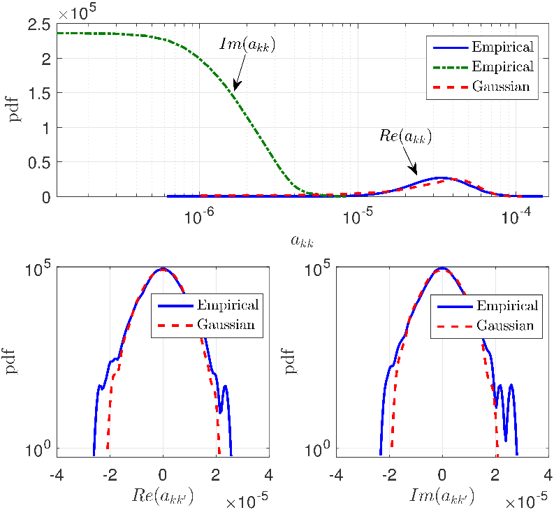
Under the assumption that is Gaussian distributed, in (16) becomes the MMSE estimate of . As a consequence, and are independent. In addition, by following a similar methodology as in (20) and (21), we can show that any linear combination of and are asymptotically (for large ) Gaussian distributed, and hence and are asymptotically jointly Gaussian distributed. Furthermore, and are uncorrelated so they are independent. Hence, the achievable downlink rate (19) is reduced to33 3 A formula similar to (22) but for co-located massive MIMO systems, was given in [9, 10] with equality between the left and right hand sides. Those expressions were not rigorously correct capacity lower bounds (although very good approximations), as is non-Gaussian in general.
| (22) |
Proposition 2: With conjugate beamforming, an achievable rate of the transmission from the APs to the th user is
| (23) |
Proof:
See Appendix B. ∎
IV Numerical Results
We compare the performance of cell-free massive MIMO for three different assumptions on CSI: (i) Statistical CSI, without downlink pilots and users exploiting only statistical knowledge of the channel gain [2]; (ii) Beamforming Training, transmitting downlink pilots and users estimating the gain from those pilots; (iii) Perfect CSI, where the users know the effective channel gain. The latter represents an upper bound (genie) on performance, and is not realizable in practice. The gross spectral efficiencies for these cases are given by (24) at the top of the page.
Taking into account the performance loss due to the downlink and uplink pilots, the per-user net throughput (bit/s) is
| (25) |
where is the bandwidth, is the length of the coherence interval in samples, and is the pilots overhead, i.e., the number of samples per coherence interval spent for the training phases.
We further examine the performance improvement by using the max-min fairness power control algorithm in [2], which provides equal and hence uniformly good service to all users for the Statistical CSI case. When using this algorithm for the Beamforming Training case (and for the Perfect CSI bound), we use the power control coefficients computed for the Statistical CSI case. This is, strictly speaking, not optimal but was done for computational reasons, as the rate expressions with user CSI are not in closed form.
IV-A Simulation Scenario
Consider APs and users uniformly randomly distributed within a square of size . The large-scale fading coefficient is modeled as
| (26) |
where represents the path loss, and is the shadowing with standard deviation and . We consider the three-slope model for the path loss as in [2] and uncorrelated shadowing. We adopt the following parameters: the carrier frequency is 1.9 GHz, the bandwidth is 20 MHz, the shadowing standard deviation is 8 dB, and the noise figure (uplink and downlink) is 9 dB. In all examples (except for Figures 4 and 5) the radiated power (data and pilot) is 200 mW for APs and 100 mW for users. The corresponding normalized transmit SNRs can be computed by dividing radiated powers by the noise power, which is given by
where is the Boltzmann constant, and (Kelvin) is the noise temperature. The AP and user antenna height is 15 m, 1.65 m, respectively. The antenna gains are dBi. Lastly, we take , and samples which corresponds to a coherence bandwidth of 200 kHz and a coherence time of 1 ms. To avoid cell-edge effects, and to imitate a network with an infinite area, we performed a wrap-around technique, in which the simulation area is wrapped around such that the nominal area has eight neighbors.
IV-B Performance Evaluation
We focus first on the performance gain, over the conventional scheme, provided by jointly using Beamforming Training scheme and max-min fairness power control in the downlink. We consider two scenarios, with different network densities.

Figure 2 shows the cumulative distribution function (cdf) of the per-user net throughput for the three cases, with , . In such a low density scenario, the channel hardening is less pronounced and performing the Beamforming Training scheme yields high performance gain over the statistical CSI case. Moreover, the Beamforming Training curve approaches the upper bound. Combining max-min power control with Beamforming Training scheme, gains can be further improved. For instance, Beamforming Training provides a performance improvement of over the statistical CSI case in terms of 95%-likely per-user net throughput, and in terms of median per-user net throughput.
By contrast, for higher network densities the gap between statistical and Beamforming Training tends to be reduced due to two factors: as increases, the statistical CSI knowledge at the user side is good enough for reliable downlink detection due to the channel hardening; as increases, the pilot overhead becomes significant. In Figure 3 the scenario with , is illustrated. Here, the 95%-likely and the median per-user net throughput of the Beamforming Training improves of and , respectively, the performance of the statistical CSI case.

Max-min fairness power control maximizes the rate of the worst user. This philosophy leads to two noticeable consequences: the curves describing with power control are more concentrated around their medians; as increases, performing power control has less impact on the system performance, since the probability to have users experiencing poor channel conditions increases.
Finally, we compare the performance provided by the two schemes by setting different values for the radiated powers. In Figure 4, the radiated power is set to 50 mW and 20 mW for the downlink and the uplink, respectively, with and . In low SNR regime, with max-min fairness power control, Beamforming Training scheme outperforms the statistical CSI case of about in terms of 95%-likely per-user net throughput, and about in terms of median per-user net throughput.

Similar performance gaps are obtained by increasing the radiated power to 400 mW for the downlink and 200 mW for the uplink, as shown in Figure 5.

V Conclusion
Co-located massive MIMO systems do not need downlink training since by virtue of channel hardening, the effective channel gain seen by each user fluctuates only slightly around its mean. In contrast, in cell-free massive MIMO, only a small number of APs may substantially contribute, in terms of transmitted power, to serving a given user, resulting in less channel hardening. We showed that by transmitting downlink pilots, and performing Beamforming Training together with max-min fairness power control, performance of cell-free massive MIMO can be substantially improved.
We restricted our study to the case of mutually orthogonal pilots. The general case with non-orthogonal pilots may be included in future work. Further work may also include pilot assignment algorithms, optimal power control, and the analysis of zero-forcing precoding technique.
Appendix
V-A Proof of Proposition 1
- •
Compute :
From (11), and by using , we have
(27) Owing to the properties of MMSE estimation, and are independent, . Therefore,
(28) - •
V-B Proof of Proposition 2
References
- [1] T. L. Marzetta, “Noncooperative cellular wireless with unlimited numbers of base station antennas,” IEEE Trans. Wireless Commun., vol. 9, no. 11, pp. 3590–3600, Nov 2010.
- [2] H. Q. Ngo, A. E. Ashikhmin, H. Yang, E. G. Larsson, and T. L. Marzetta, “Cell-free massive MIMO versus small cells,” IEEE Trans. Wireless Commun., 2016, submitted. [Online]. Available: http://arxiv.org/abs/1602.08232
- [3] E. Nayebi, A. Ashikhmin, T. L. Marzetta, and H. Yang, “Cell-free massive MIMO systems,” in Proc. Asilomar Conference on Signals, Systems and Computers, Nov 2015, pp. 695–699.
- [4] K. T. Truong and R. W. Heath, “The viability of distributed antennas for massive MIMO systems,” in Proc. Asilomar Conference on Signals, Systems and Computers, Nov 2013, pp. 1318–1323.
- [5] S. Zhou, M. Zhao, X. Xu, J. Wang, and Y. Yao, “Distributed wireless communication system: a new architecture for future public wireless access,” IEEE Commun. Mag., vol. 41, no. 3, pp. 108–113, Mar 2003.
- [6] J. Vieira, F. Rusek, and F. Tufvesson, “Reciprocity calibration methods for massive MIMO based on antenna coupling,” in Proc. IEEE Global Communications Conference (GLOBECOM), Dec 2014, pp. 3708–3712.
- [7] J. Hoydis, S. ten Brink, and M. Debbah, “Massive MIMO in the UL/DL of cellular networks: How many antennas do we need?” IEEE J. Sel. Areas Commun., vol. 31, no. 2, pp. 160–171, Feb 2013.
- [8] E. Björnson, E. G. Larsson, and M. Debbah, “Massive MIMO for maximal spectral efficiency: How many users and pilots should be allocated?” IEEE Trans. Wireless Commun., vol. 15, no. 2, pp. 1293–1308, Feb 2016.
- [9] H. Q. Ngo, E. G. Larsson, and T. L. Marzetta, “Massive MU-MIMO downlink TDD systems with linear precoding and downlink pilots,” in Proc. Allerton Conference on Communication, Control, and Computing, Oct 2013, pp. 293–298.
- [10] A. Khansefid and H. Minn, “Achievable downlink rates of MRC and ZF precoders in massive MIMO with uplink and downlink pilot contamination,” IEEE Trans. Commun., vol. 63, no. 12, pp. 4849–4864, Dec 2015.
- [11] J. Zuo, J. Zhang, C. Yuen, W. Jiang, and W. Luo, “Multi-cell multi-user massive MIMO transmission with downlink training and pilot contamination precoding,” IEEE Trans. Veh. Technol., vol. PP, no. 99, pp. 1–1, Sep 2015.
- [12] S. M. Kay, Fundamentals of Statistical Signal Processing: Estimation Theory. Englewood Cliffs, NJ: Prentice Hall, 1993.
- [13] M. Medard, “The effect upon channel capacity in wireless communications of perfect and imperfect knowledge of the channel,” IEEE Trans. Inf. Theory, vol. 46, no. 3, pp. 933–946, May 2000.