A FORM OF MULTIVARIATE PARETO DISTRIBUTION WITH APPLICATIONS TO FINANCIAL RISK MEASUREMENT
Jianxi Su and Edward Furman11 1 Corresponding author. Department of Mathematics and Statistics, York University, Toronto, Ontario M3J 1P3, Canada; E-mail: efurman@mathstat.yorku.ca; Tel: 416-736-2100 Ext 33768; Fax: 416-736-5757.
Department of Mathematics and Statistics, York University,
Toronto, Ontario M3J 1P3,
Canada
Abstract. A new multivariate distribution possessing arbitrarily parame-
trized and positively dependent univariate Pareto margins is introduced. Unlike the probability law of Asimit et al. (2010) [Asimit, V., Furman, E. and Vernic, R. (2010) On a multivariate Pareto distribution. Insurance: Mathematics and Economics 46(2), 308 – 316], the structure in this paper is absolutely continuous with respect to the corresponding Lebesgue measure. The distribution is of importance to actuaries through its connections to the popular frailty models, as well as because of the capacity to describe dependent heavy-tailed risks. The genesis of the new distribution is linked to a number of existing probability models, and useful characteristic results are proved. Expressions for, e.g., the decumulative distribution and probability density functions, (joint) moments and regressions are developed. The distributions of minima and maxima, as well as, some weighted risk measures are employed to exemplify possible applications of the distribution in insurance.Keywords and phrases: Multivariate Pareto distributions, characterizations, dependence, weighted risk measures, minima, maxima.
1. introduction
At the outset, we fix the probability space and define the random vector (r.v.) as a map from to the -dimensional Borel space . The cumulative distribution function (c.d.f.) of is in the sequel denoted by , and the corresponding probability density function (p.d.f.) by , where . Finally, and denote, respectively, the marginal c.d.f. and p.d.f. of . Clearly, when the coordinates of are stochastically independent, then there is only one way to formulate the c.d.f. , whereas the shapes of the just-mentioned c.d.f. are infinite otherwise.
We further discuss the so-called multivariate reduction approach to creating random vectors with dependent coordinates. This paves the way to introducing the main object of our interest in Section 2. For applications of the multivariate reduction method in insurance, we refer to, e.g., Vernic (1997, 2000), Pfeifer and Nešlehová (2004), Furman and Landsman (2005, 2010), Boucher et al. (2008) and Tsanakas (2008), as well as to the references therein.
Let be an -variate r.v. with mutually independent univariate margins distributed gamma. Namely, for , the p.d.f. of is given by
| (1.1) |
with the corresponding Laplace transform being well-defined on (the interval of interest herein) and given by
| (1.2) |
Definition 1.1 (Furman, 2008; Furman and Landsman, 2010).
Let denote a deterministic matrix with suitable non-negative entries. Then is distributed -variate gamma with shape parameters and rate parameters for appropriate positive Borel functions . Succinctly, we write , where and are vectors of parameters.
Example 1.1 (Mathai and Moschopoulos, 1991; see also Cherian, 1941 and Ramabhadran, 1951).
Let be mutually independent random variables distributed gamma with arbitrary parameters, and choose the matrix such that, for and , it holds that , and zero otherwise. Then , where and are two -variate vectors of parameters.
Example 1.2 (Mathai and Moschopoulos, 1992; see also, Furman, 2008).
Let , be mutually independent random variables distributed gamma with arbitrary parameters, and choose the matrix such that, for and , it holds that and zero otherwise. Then , where and are two -variate vectors of parameters.
Example 1.3 (Furman, 2008).
Let be again mutually independent random variables distributed gamma with arbitrary parameters, and choose the matrix such that, for and , it holds that , and zero otherwise. Then , where and are two -variate vectors of parameters.
In the sequel, we embark on the idea in Example 1.3 to introduce an encompassing yet tractable multivariate distribution with univariate margins distributed Pareto. We note in passing that a real-valued r.v. is said to be distributed Pareto of the nd kind, succinctly where is a location parameter, is a scale parameter and is a tail index, if its c.d.f. is given by
| (1.3) |
(see, e.g., Pareto, 1897; Arnold, 1983; Kotz et al., 2000). Similarly to Asimit et al. (2010), we set , which conveniently makes the support of the distribution coincide with the positive half of the real line, i.e., and does not lead to any loss of generality. The resulting distribution (Lomax distribution), notationally , enjoys a great variety of applications in all areas of applied mathematics in general and in actuarial science in particular, as it naturally arises in the extreme value theory as the limiting distribution of the excess-of-loss r.v. where denotes a threshold (see, e.g., Balkema and de Haan, 1974; Pickands, 1975).
The rest of the paper is organized as follows. In Section 2 a multivariate probability structure with dependent Pareto-distributed univariate margins is introduced and linked to a number of existing multivariate models. Then distributional properties of the new structure are derived and some characterization results are proved in Sections 2 and 3. In Section 4 the new multivariate Pareto is reintroduced as a variant of the minima-based multiple risk factor model, and some applications to notions of actuarial interest are considered. In Section 5 an application of the model is elucidated with the help of a numerical example borrowed from the context of default risk. Section 6 concludes the paper. All proofs are relegated to the appendix to facilitate the reading.
2. New multivariate Pareto distribution
Let be a r.v. with mutually independent coordinates , and choose the matrix such that , where are deterministic constants, , and . The following definition unifies Examples 1.1, 1.2 and 1.3 and serves as an auxiliary tool for constructing the multivariate Pareto distribution of interest.
Definition 2.1.
Let , then it follows an -variate gamma distribution, notationally , where with and are two vectors of parameters.
We note in passing that Definition 2.1 (auxiliary for the present paper) establishes an encompassing multivariate probability law with gamma-distributed univariate margins and an additive background risk dependence structure (see, Gollier and Pratt, 1996; Tsanakas, 2008; Furman and Landsman, 2010 for applications of the additive background risk models in economics and actuarial science). More specifically, the following simple special cases of readily recover the models of, respectively, Mathai and Moschopoulos (1991, 1992) and Furman (2008):
- •
for and zero otherwise - Example 1.1;
- •
for and zero otherwise - Example 1.2;
- •
for and zero otherwise - Example 1.3.
Some elementary but useful properties of follow directly by definition or from the Laplace transform that is established next.
Proposition 2.1.
Let be the r.v. distributed multivariate gamma as in Definition 2.1, then the corresponding Laplace transform is given by
and it is well-defined on .
Immediate consequences of Proposition 2.1 are, for , that
- •
the distribution of is ‘marginally closed’, i.e., ;
- •
the expectation of the -th coordinate is ;
- •
the variance of the -th coordinate is ;
- •
for , the covariance between the coordinates and is non-negative and given by
- •
for , the Pearson linear correlation between the coordinates and is non-negative and given by
We are now in a position to introduce the multivariate Pareto distribution of interest. In fact, simple observation (1.2) along with Proposition 2.1 result in the following definition.
Definition 2.2.
We call the r.v. having the decumulative distribution function (d.d.f.)
| (2.1) |
a multivariate Pareto of the nd kind. Succinctly, we write , where are two deterministic vectors of positive parameters, and and are scalar-valued and matrix-valued parameters, respectively.
Generally, distributions with Paretian tails have been applied in a multitude of areas. Herein we refer to: Benson et al. (2007) for applications in modelling catastrophic risk; Koedijk et al. (1990), Longin (1996), Gabaix et al. (2003) for applications in general financial phenomena; Cebrián et al. (2003) for applications in insurance pricing; and Soprano et al. (2010), Chavez-Demoulin et al. (2015) for applications in risk management.
Specifically, the probability law in Definition 2.2 is a generalization of the classical multivariate Pareto distribution of Arnold (1983) with the d.d.f. . Indeed, set in (2.1) and obtain, for , that
| (2.2) |
That being said, unlike the classical multivariate Pareto distribution of Arnold (1983), the structure in Definition 2.2 incorporates stochastic independence - set and zero otherwise and obtain, for denoting the d.d.f. of a multivariate Pareto with independent margins, that
Consequently, the new multivariate Pareto distribution meaningfully fills the gap between the multivariate probability distributions with independent and Arnold-dependent Pareto-distributed margins.
In addition, unlike (2.2), allows for distinct marginal tail indices (see, Proposition 2.2 below). Furthermore, the new multivariate Pareto distribution unifies the probability models studied recently in Chiragiev and Landsman (2009). Namely, in order to obtain their ‘flexible Pareto type I and II’ we choose and zero otherwise and for and zero otherwise, respectively.
Lastly but perhaps most importantly in actuarial applications, d.d.f. (2.1) admits stochastic representations that mimic the multiplicative background risk model (Franke et al., 2006) and the minima-based common shock model (Bowers et al., 1997) (see, respectively, Theorems 2.2 and 4.1 in this paper). Stochastic representations are a very welcome facet, since they endow probabilistic models with an important feature of interpretability, and as a result contribute greatly to the process of model selection and implementation.
We further document several simple properties of the multivariate Pareto with d.d.f. (2.1). The proofs are straightforward and thus omitted.
Proposition 2.2.
Let as in Definition 2.2, then, for , the marginal d.d.f. of is
that is , where . Also, for and setting , we have that
| (2.3) |
and furthermore setting , we obtain that
| (2.4) |
In Proposition 2.2, the substitution and zero otherwise yields Theorem 1 of Chiragiev and Landsman (2009), whereas the substitution for and zero otherwise results in their Theorem 5.
In what follows, we develop an expression for the joint p.d.f. of the multivariate Pareto distribution of interest. To this end, let
| (2.5) |
where establishes a set of positive integer indices such that , and are appropriately chosen constants. Also, let
denote the Pochhammer symbol.
Theorem 2.1.
Let as in Definition 2.2, then the corresponding joint p.d.f. is formulated, for , as
| (2.6) |
where are appropriately chosen constants and .
In general, the constants can be rather involved. For an insight, we show how (2.6) reduces to the p.d.f. of the classical multivariate Pareto distribution of Arnold (1983). To this end, set for and . Then from (2.5), we have that
with the right-hand side denoting the multinomial coefficient. On the other hand, as (2.6) must integrate to one and since for the Arnold’s multivariate Pareto distribution, we have, for , that
we obtain
as required.
The following theorem establishes a useful characteristic relation in the context of the multivariate Pareto distribution of interest, and it also plays an important role when deriving the formula for the corresponding Pearson linear correlation (see, Theorem 3.1 in Section 3). In the sequel ‘’ denotes equality in distribution.
Theorem 2.2.
Let be a r.v. with independent and exponentially-distributed univariate margins , and denote by the -variate gamma distribution introduced in Definition 2.1; here with , and are vectors of parameters. Assume that and are stochastically independent, then has d.d.f. (2.1), and it is thus the -variate Pareto distribution introduced in Definition 2.2 if and only if .
Theorem 2.2 establishes the multiplicative background risk representation of the multivariate probabilistic structure of main interest herein (see, Franke et al., 2006; Meyers, 2007, Asimit et al., 2013, 2016 for applications of the multiplicative background risk models in economics and actuarial science).
We conclude this section with yet another characterization of the multivariate Pareto distribution of interest and its two implications. Namely, let and denote, respectively the minima and the maxima r.v.’s, and let be univariate coordinates of the multivariate Pareto r.v. of interest in this paper.
Theorem 2.3.
Let be distributed as per Definition 2.2, then admits the mixture representation as and , where are univariate mutually independent r.v.’s distributed gamma.
An important corollary of Theorem 2.3 is a random parameter representation (see, e.g., Feller, 1966) of the d.d.f.’s of and . The following lemma is crucial in studying the distribution of in Theorem 2.4.
Lemma 2.1 (Moschopoulos, 1985; Furman and Landsman, 2005).
For , let denote independent gamma-distributed r.v.’s. Then the distribution of is gamma with a random shape parameter. More specifically, where , and is an integer-valued non-negative r.v. with the probability mass function (p.m.f.) given by
| (2.7) |
where
and
Theorem 2.4.
While Theorem 2.4 demonstrates that the minima r.v. is distributed mixed Pareto with random tail index parameter, the next theorem asserts that the maxima r.v. has a d.d.f. that is a linear combination of the d.d.f.’s of such mixed Pareto-distributed r.v.’s. The proof is similar to the one of Proposition 2 in Vernic (2011) and is thus omitted.
Theorem 2.5.
3. Bivariate quantities of interest
It is worthwhile to make an additional observation before stating the main result of this section. Namely, we note in passing that for , a r.v. distributed the bivariate gamma per Definition 2.1 and an -variate r.v. having mutually independent coordinates , the following stochastic representation holds
| (3.1) |
where , and are mutually independent gamma-distributed r.v.’s with the shape parameters , and , respectively.
We next show that the covariance of a random couple within the multivariate Pareto of interest in this paper can be formulated using the hypergeometric function (see, Gradshteyn and Ryzhik, 2007), which is formulated as
| (3.2) |
where . For all positive, and these are the cases of interest in the present paper, the radius of convergence of the series is the open disk . On the boundary , the series converges absolutely if , and it converges except at if .
Theorem 3.1.
Let as in Definition 2.2 and assume that both and exceed two, then, for ,
An immediate consequence of Theorem 3.1 is that the maximal attainable Pearson correlation in the context of the multivariate Pareto distribution introduced in the present paper is not one. This consequence is however solely a result of the fact that the Pearson index of correlation exists only if the involved second moments are finite, a pitfall that is well-known to non-life actuaries, which often deal with heavy-tailed losses (see, Embrechts et al., 2002).
Corollary 3.1.
Let and assume that both and exceed two for , then, for the Pearson correlation, it holds that .
Another consequence of Theorem 3.1 pertains to two special cases of the multivariate Pareto introduced in this paper, and it is formulated as the following corollary.
Corollary 3.2.
Let and be distributed, respectively, the multivariate flexible Pareto of type and of Chiragiev and Landsman (2009). Then the corresponding covariances are readily obtained, for , as
| (3.3) | |||||
for and , and as
| (3.4) |
for and .
We note in passing that expression (3.4) confirms the one derived in Chiragiev and Landsman (2009), whereas formula (3.3) complements the discussion therein. Also, the covariance of two r.v.’s coming from the Arnold’s multivariate Pareto distribution (see, Arnold, 1983) is readily obtained from both (3.3) and (3.4). More specifically, we set for all and verify that (3.3) reduces to
for . The verification is straightforward in the case of (3.4).
Generalized hypergeometric function (3.2) plays an important role when deriving the centred regression function , where (see, Furman and Zitikis, 2008b, 2010, for applications of the function in insurance and finance). We next present the conditional d.d.f., followed by the centered regression function for a pair of r.v.’s having the probability law as in Definition 2.2. To this end, let
Theorem 3.2.
Theorem 3.3.
Let as in Definition 2.2, the centred regression function of on , is given, for , by
| (3.6) |
where
The centred regression function is monotonically-increasing and concave.
We reiterate that our results readily recover the ones derived in Landsman and Chiragiev (2009). More specifically, by a simple alignment of notation in Theorem 3.3 above, we obtain Theorem 3 in loc. cit., whereas by choosing in Theorem 3.3 and hence for
we end up with Theorem 7 therein.
Clearly, the centred regression function of the new multivariate Pareto distribution is not linear, while it is well-known that the classical multivariate Pareto has linear regression (see, Arnold, 1983). Theorem 3.3 confirms the latter fact by setting and in (3.6), which then reduces to the following linear form
for and .
4. Applications to insurance
In what follows, we assume that denotes a risk portfolio (r.p.) with representing its risk components (r.c.’s). According to Theorem 2.2, if , then it admits the multiplicative background risk representation (see, Franke et al., 2006; Meyers, 2007; Asimit et al., 2013, 2016).
We next show that the new multivariate Pareto distribution can also be interpreted as a variant of the classical minima-based common shock model (see, e.g., Bowers et al, 1997). To this end, assume that the -th r.c of the r.p. is exposed to the set , of risk factors (r.f.’s) and let the r.v. stipulate the randomness of actuarial interest associated with the r.f.’s. The following theorem establishes the minima-based multiple risk factor representation of the multivariate Pareto proposed in the present paper. We note in passing that ‘’ stands for the mixture operator, i.e., given two appropriately jointly measurable r.v.’s and , it holds that .
Theorem 4.1.
Let be r.v.’s with independent exponentially-distributed margins , and let be a deterministic matrix of zero-one coefficients. Also, let be a r.v. having independent gamma-distributed margins with arbitrary shape parameters and rate parameters equal to , . Set, for and ,
| (4.1) |
then .
Theorem 4.1 suggests that the multivariate Pareto distribution proposed in the present paper might be an appropriate formal framework for modelling dependent default, survival or failure times when these times are exponentially-distributed with random parameters. We elaborate on this observation in Section 5.
4.1. Actuarial risk measurement
Regulatory accords around the globe require that insurance companies carry out a careful assessment of their future losses. From now on, the r.v. is interpreted as an insurance loss r.v., and denotes the collection of such r.v.’s.
Definition 4.1.
A risk measure is a functional map .
The literature on risk measures is vast and growing quickly. The following two indices are arguably the most popular amongst practitioners.
Definition 4.2.
Let and fix , then the Value-at-Risk (VaR) and the Conditional Tail Expectation (CTE) risk measures are respectively given by
| (4.2) |
and
| (4.3) |
We note in passing that both VaR and CTE are distorted as well as weighted risk measures (see, respectively, Wang, 1996; and Furman and Zitikis, 2008a).
Definition 4.3.
Furman and Zitikis (2008a), see also Choo and de Jong (2009, 2010). Let be a non-decreasing Borel (weight) function, such that , then the class of weighted risk measures is defined as
| (4.4) |
Let be two legitimate weight functions such that all expectations in (4.5) are finite, and consider a generalized variant of (4.4)
| (4.5) |
Proposition 4.1.
Let and assume that , then for any legitimate weight function, the functional admits representation (4.5).
Corollary 4.1.
Let as in Definition 2.2, then, for and , we have that
Corollary 4.2.
Let and assume that , then the CTE risk measure of is, if exists and for , given by
where .
Corollary 4.3.
Let as in Definition 2.2, we have that the CTE risk measure is, if exists and for and , given by
| (4.6) | |||||
where .
The minima r.v. plays an important role in insurance mathematics (recall, e.g., the joint life policies in life insurance), as well as in general finance (think of, e.g., the first-to-default baskets).
Recall that the r.v. has been defined as an integer-valued non-negative r.v. with the following p.m.f.
| (4.7) |
where
and
Proposition 4.2.
In the context of the multivariate Pareto of interest, the CTE risk measure of the minima can be written, if finite and for , as
where , where , and is an integer-valued r.v. with the p.m.f. obtained from the p.m.f. of with the help of the following change of measure
| (4.8) |
Proposition 4.3.
In the context of the multivariate Pareto of interest, the CTE risk measure of the maxima can be written, if finite and for , as the following linear combination
where and .
Definition 4.4 (Furman and Zitikis, 2008b).
Let be a non-decreasing Borel function, such that , then the functional is referred to as the economic risk measure. Moreover, the special form of , given by
| (4.9) |
is called a weighted economic risk measure.
We further derive an expression for the economic CTE risk measure, which is a particular case of (4.9) with and . To this end, we find the next proposition useful. The proof is plain and thus omitted.
Proposition 4.4.
Proposition 4.5.
In the context of the multivariate Pareto of interest, the economic CTE risk measure is given, for , and , by
To summarize, so far we have introduced and studied a new multivariate probability distribution with the univariate margins distributed Pareto of the 2nd kind. The dependence structure of the new distribution is driven by a number of stochastic representations that are variants of the multiplicative background risk and the minima-based common shock models. We next employ the latter interpretation of the proposed multivariate probability distribution to exemplify its possible application to modelling and measuring default risk.
5. Numerical illustration
For the sake of the discussion in this section, we adopt the view of the Financial Stability Board and the International Monetary Fund that the systemic risk can be caused by impairment of all or parts of the financial system, and more formally, we call the risk factor ‘systemic’, if for at least two distinct r.c.’s . Similarly, we call the risk factor ‘idiosyncratic’, if for only one risk component .
Consider obligors in a default risk portfolio, each of which is exposed to exactly two distinct categories of fatal risk factors, e.g., systemic (category A) and idiosyncratic (category B). We assume that the risk factors from distinct risk categories are independent and that the hitting times (or occurrences) of defaults of the r.c.’s are exponentially-distributed with random parameters distributed gamma. In fact, the future lifetime r.v. of the -th r.c. has exponential distribution with the random parameter , where are distributed gamma with unit rate parameters, and is or 3. Then Theorem 4.1 readily implies that the joint default times of the aforementioned r.c.’s has d.d.f. (2.1).
To illustrate the effect of the dependence structure on the joint default probability we further set the dimension to and specialize the set-up above along the lines in Section 16.8 of Engelmann and Rauhmeier (2011) as well as employing the 2014’s Annual Global Corporate Default Study and Rating Transitions of Standard & Poor’s. (Standard & Poor’s, 2015). More specifically, we set , fix the time horizon to years and choose the corresponding default probability, say, to be equal to (on par with the ‘B’ credit rating of speculative entities). This yields the multivariate probability structure of Definition 2.2 with identically distributed margins having the parameters and , for and .
Then we explore three different exposures of the obligors to the systemic and idiosyncratic r.f.’s. The distinct exposures are stipulated by appropriate choices of the parameters gathered by matrices . We compare the aforementioned three exposures with the reference case in which no systemic risk presents, that is the joint d.d.f. of default times is a trivariate Pareto with independent margins. We note in passing that the expressions for the d.d.f.’s below readily follow from Theorem 4.1, whereas the values of the Pearson correlation coefficient are in non-trivial cases obtained with the help of Theorem 3.1.
- Case (1).
Only the systemic risk presents, and all risk components are exposed to it. The exposure is represented schematically with the use of the following matrix, in which the rows and the columns represent r.c.’s and r.f.’s, respectively
The joint d.d.f. of the risk components is given by
where are all in . This is obviously the d.d.f. of the classical trivariate Pareto distribution (Arnold, 1983). In this r.p., the Pearson correlation coefficient between any two of the r.c.’s is .
In the following two cases, both the systemic and idiosyncratic risks present.
- Case (2).
There are overall three uncorrelated idiosyncratic risk factors and one systemic risk factor. The exposure is gathered by the following block matrix
The joint d.d.f. of the risk components is given by
where are all in . This case corresponds to the ‘flexible Pareto type I’ of Landsman and Chiragiev (2009). In this r.p., the Pearson correlation coefficient between any two of the r.c.’s is .
- Case (3).
The systemic risk is represented by two distinct risk factors of which one targets the entire risk portfolio and the other only hits r.c.’s and . There is one idiosyncratic risk factor, and only r.c. is exposed to it. The exposure block matrix is given by
The joint d.d.f. of the risk components is
where are all in . In this r.p., the Pearson correlation coefficient between r.c. #1 and #2 is , and it is equal to otherwise.
5.1. Expected times of the first default
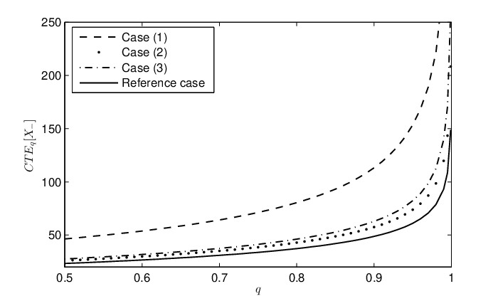
The left panel of Figure 1 depicts the values of for , and portfolios (1) to (3) as well as the reference portfolio, denoted by . As the risk components are identically distributed, it is not difficult to see that the following ordering holds
| (5.1) |
where ‘’ denotes first order stochastic dominance (FSD). Furthermore, since the CTE risk measure is known to preserve the FSD ordering, we also have that
for all and . This conforms with Figure 1 (left panel), which hints that the r.p.’s with more significantly correlated r.c.’s enjoy higher, and thus more favourable, occurrence times of the first default.
The downside of high correlations is elucidated in Figure 2, in which we leave the probability of default to be equal to (‘B’ rating), but vary the parameter that stipulates the effect of the risk factors. In this respect, we observe that the r.p.’s with stronger correlations between r.c.’s are more sensitive to the changes in the parameter, and therefore such r.p.’s must be monitored and stress-tested more frequently.


5.2. Expected times of the last default
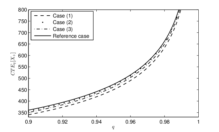
Figure 1 (right panel) depicts the values of for and portfolios (1) to (3) as well as the reference portfolio . Evoking Theorem 2.5 along with (5.1) results in
and hence
for all and . This conforms with the right panel of Figure 1.
Unlike in the case of the first default, we observe that if the time of the last default is of interest and the distributions of the r.c.’s are fixed, then assuming stronger correlations between r.c.’s yields a more conservative assessment of the expected time of the last default.
6. Conclusions
We have introduced and studied a new form of an absolutely continuous with respect to the Lebesgue measure multivariate probability law with the univariate margins distributed Pareto of the 2nd kind. The genesis of our distribution is threefold, i.e., it originates as the Laplace transform of a multivariate gamma distribution with the dependence structure based on the additive form of the multivariate reduction method, and it also admits variants of the multiplicative background risk model as well as the minima-based common shock model. We have meaningfully positioned the proposed multivariate Pareto distribution in the general context of the current state of the art. We have proved and employed certain characteristic results to derive, e.g., the (conditional/product) moments of the new multivariate Pareto as well as the distributions of minima and maxima. Last but not least, we have developed expressions for some tail-based risk measures of actuarial interest and elucidated our findings with the help of a numerical example.
Acknowledgements
We thank the anonymous referees and the Associate Editor, Prof. Montserrat Guillén, for valuable comments and suggestions that improved the work significantly and resulted in a better presentation of the material. We are also grateful to Prof. Paul Embrechts and all participants of the ETHs Series of Talks in Financial and Insurance Mathematics for feedback and insights.
Our research has been supported by the Natural Sciences and Engineering Research Council (NSERC) of Canada. Jianxi Su also acknowledges the financial support of the Government of Ontario and MITACS Canada via, respectively, the Ontario Graduate Scholarship program and the Elevate Postdoctoral fellowship.
References
Arnold, B.C. (1983) Pareto Distributions. International Cooperative Publishing House, Fairland.
Asimit, V., Furman, E. and Vernic, R. (2010) On a multivariate Pareto distribution. Insurance: Mathematics and Economics 46(2), 308 – 316.
Asimit, V., Vernic, R. and Zitikis, R. (2013) Evaluating risk measures and capital allocations based on multi-losses driven by a heavy-tailed background risk: The multivariate Pareto-II model. Risk 1(1), 14 – 33.
Asimit, V., Vernic, R. and Zitikis, R. (2016) Background risk models and stepwise portfolio construction. Methodology and Computing in Applied Probability, in press.
Balkema, A. and de Haan, L. (1974) Residual life time at great age. Annals of Probability 2(5), 792 – 804.
Benson, D.A., Schumer, R. and Meerschaert, M.M. (2007) Recurrence of extreme events with power-law interarrival times. Geophysical Research Letters 34(16), 1 – 5.
Boucher, J.P., Denuit, M. and Guillén, M. (2008) Models of insurance claim counts with time dependence based on generalization of Poisson and negative binomial distributions. Variance 2(1), 135 – 162.
Bowers, N.L., Gerber, H.U., Hickman, J.C., Jones, D.A. and Nesbitt, C.J. (1997) Actuarial Mathematics. Second edition. Society of Actuaries, Schaumburg.
Cebrián, A.C., Denuit, M. and Lambert, P. (2003) Generalized Pareto fit to the Society of Actuaries large claims database. North American Actuarial Journal 7(3), 18 – 36.
Chavez-Demoulin, V., Embrechts, P. and Hofert, M. (2015) An extreme value approach for modeling operational risk losses depending on covariates. Journal of Risk and Insurance, in press.
Cherian, K.C. (1941) A bivariate correlated gamma-type distribution function. Journal of the Indian Mathematical Society 5, 133 – 144.
Chiragiev, A. and Landsman, Z. (2009) Multivariate flexible Pareto model: Dependency structure, properties and characterizations. Statistics and Probability Letters 79(16), 1733 – 1743.
Choo, W. and de Jong, P. (2009) Loss reserving using loss aversion functions. Insurance: Mathematics and Economics 45(2), 271 – 277.
Choo, W. and de Jong, P. (2010) Determining and allocating diversification benefits for a portfolio of risks. ASTIN Bulletin 40(1), 257 – 269.
Embrechts, P., McNeil, A. and Straumann, D. (2002) Correlation and dependence in risk management: Properties and pitfalls. In: Dempster, M. et al. (Eds), Risk Management: Value at Risk and Beyond. Cambridge University Press, Cambridge.
Engelmann, B. and Rauhmeier, R. (2011) The Basel II Risk Parameters: Estimation, Validation, Stress Testing - with Applications to Loan Risk Management. Springer, Berlin.
Feller, W. (1966) An Introduction to Probability Theory and its Applications. John Wiley and Sons, New York.
Franke, G., Schlesinger, H. and Stapleton, R.C. (2006) Multiplicative background risk. Management Science 52(1), 146 – 153.
Furman, E. (2008) On a multivariate gamma distribution. Statistics and Probability Letters 78(15), 2353 – 2360.
Furman, E. and Landsman, Z. (2005) Risk capital decomposition for a multivariate dependent gamma portfolio. Insurance: Mathematics and Economics 37(3), 635 – 649.
Furman, E. and Landsman, Z. (2010) Multivariate Tweedie distributions and some related capital-at-risk analysis. Insurance: Mathematics and Economics 46(2), 351 – 361.
Furman, E. and Zitikis, R. (2008a) Weighted premium calculation principles. Insurance: Mathematics and Economics 42(1), 459 – 465.
Furman, E. and Zitikis, R. (2008b) Weighted risk capital allocations. Insurance: Mathematics and Economics 43(2), 263 – 269.
Furman, E. and Zitikis, R. (2010) General Stein-type covariance decompositions with applications to insurance and finance. ASTIN Bulletin 40(1), 369 – 375.
Gabaix, X., Gopikrishnan, P., Plerou, V. and Stanley, H.E. (2003) A theory of power-law distributions in financial market fluctuations. Nature 423, 267 – 270.
Gollier, C. and Pratt, J.W. (1996) Weak proper risk aversion and the tempering effect of background risk. Econometrica 64(5), 1109 – 1123.
Gradshteyn, I.S. and Ryzhik, I.M. (2007) Table of Integrals, Series and Products. Seventh edition. Academic Press, New York.
Koedijk, K.G., Schafgans, M.M.A. and de Vries, C.G. (1990) The tail index of exchange rate returns. Journal of International Economics 29(1-2), 93 – 108.
Kotz, S., Balakrishnan, N. and Johnson, N.L. (2000) Continuous Multivariate Distributions. Second edition. Wiley, New York.
Longin, F.M. (1996) The asymptotic distribution of extreme stock market returns. Journal of Business 69(3), 383 – 408.
Mathai, A.M. and Moschopoulos, P.G. (1991) On a multivariate gamma. Journal of Multivariate Analysis 39(1), 135 – 153.
Mathai, A.M. and Moschopoulos, P.G. (1992) A form of multivariate gamma distribution. Annals of the Institute of Statistical Mathematics 44(1), 97 – 106.
Meyers, G.G. (2007) The common-shock model for correlated insurance losses. Variance 1(1), 40 –52.
Moschopoulos, P.G. (1985) The distribution of the sum of independent gamma random variables. Annals of the Institute of Statistical Mathematics 37, 541 – 544.
Pareto, V. (1897) The new theories of economics. Journal of Political Economy 5(4), 485 – 502.
Pfeifer, D. and Nešlehová, J. (2004) Modeling and generating dependent risk processes for IRM and DFA. ASTIN Bulletin 34(2), 333 – 360.
Pickands, J. (1975) Statistical inference using extreme order statistics. The Annals of Statistics 3(1), 119 – 131.
Ramabhadran, V. (1951) A multivariate gamma-type distribution. Journal of Multivariate Analysis 38, 213 – 232.
Soprano, A., Crielaard, B., Piacenza, F. and Ruspantini, D. (2009) Measuring Operational and Reputational Risk: A Practitioner’s Approach. Wiley, Chichester.
Standard & Poor’s (2015) Default, transition and recovery: 2014 annual global corporate default study and rating transitions. Technical report, Standard and Poor’s, New York.
Tsanakas, A. (2008) Risk measurement in the presence of background risk. Insurance: Mathematics and Economics 42(2), 520 – 528.
Vernic, R. (1997) On the bivariate generalized Poisson distribution. ASTIN Bulletin 27(1), 23 – 32.
Vernic, R. (2000) A multivariate generalization of the generalized Poisson distribution. ASTIN Bulletin 30(1), 57 – 67.
Vernic, R. (2011) Tail conditional expectation for the multivariate Pareto distribution of the second kind: Another approach. Methodology and Computing in Applied Probability 13(1), 121 – 137.
Wang, S. (1996) Premium calculation by transforming the layer premium density. ASTIN Bulletin 26(1), 71 – 92.
Appendix A Proofs
Proof of Proposition 2.1.
Proof of Theorem 2.1.
Let denote a multivariate c.d.f. with mutually independent gamma-distributed univariate margins. We have the following string of equations
where is a vector of positive parameters. The proof is completed by computing the iterated integral. ∎
Proof of Theorem 2.2.
Proof of Theorem 2.3.
For the proof, we readily have that
which establishes the mixture representation. ∎
Proof of Theorem 2.4.
Proof of Theorem 3.1.
Let denote a multivariate c.d.f. with mutually independent gamma-distributed univariate margins. We start by employing Lemma 2.2 and observation (3.1), then do change of variables and obtain that
where ‘’ holds because of the following integral representation of the Gauss hypergeometric function (Equation 3.197(5) in Gradshtein and Ryzhik, 2007)
for and all such that the integral above converges, and ‘’ follows from Equation 7.512(5) in loc. cit. This completes the proof. ∎
Proof of Corollary 3.1.
The lower bound follows by setting and both of and to exceed two. To establish the upper bound, let and and assume that exceeds two, then we have that
where the last equality holds due to Equation 9.122(1) in Gradshteyn and Ryzhik (2007), and the covariance of interest reduces to
This, along with Proposition 2.2, completes the proof. ∎
Proof of Corollary 3.2.
To obtain (3.3), we set and zero otherwise. This implies , and (see, Example 1.1). Then the result directly follows from Theorem 3.1. To establish (3.4), let for and zero otherwise. Then the desired assertion follows because
where the latter equality holds for . This completes the proof of the corollary. ∎
Proof of Theorem 3.2.
We first note that
and then write
| (A.2) | |||||
Plain simplifications complete the proof. ∎
Proof of Theorem 3.3.
Note that for the pair , stochastic representation (3.1) is of utmost generality, i.e., conditional distribution function (4.4) coincides with the one of the type I multivariate flexible Pareto model. Hence the proof is completed by evoking Theorem 3 of Chiragiev and Landsman (2009) as well as Proposition 2.2. ∎
Proof of Theorem 4.1.
Note that
and hence, for denoting the c.d.f. of the r.v. ,
which, along with (1.2), completes the proof. ∎
Proof of Proposition 4.1.
Notice that
and set and . This concludes the proof. ∎
Proof of Corollary 4.1.
Proof of Corollary 4.3.
As , we readily have that
and
and the assertion holds by Proposition 4.1. This completes the proof. ∎
Proof of Proposition 4.2.
We readily have that
where ‘’ follows because of Corollary 2.4 and ‘’ holds since
This completes the proof. ∎