Journal: arXiv.org for the record as a manuscript.
MAREK A. SUCHENEK
Address: California State University Dominguez Hills,
Department of Computer Science,
1000 E. Victoria St., Carson, CA 90747, USA,
Suchenek@csudh.edu
Abstract
An exact formula
where
for the minimum number of comparisons of keys performed by on an -element array is derived and analyzed. The said formula is less complex than any other known formula for the same and can be evaluated in time, where is a constant. It is shown that there is no closed-form formula for the above. Other variants for are described as well.
Since the recurrence relation for the minimum number of comparisons of keys for is identical with a recurrence relation for the number of 1s in binary expansions of all integers between and (exclusively), the above results extend to the sum of binary digits problem.
Keywords:
MergeSort , sum of digits , sorting , best case.
2010 MSC
68W40 Analysis of algorithms ,
2010 MSC
11A63 Radix representation
ACM Computing Classification Theory of computation: Design and analysis of algorithms: Data structures design and analysis: Sorting and searching
Mathematics of computing: Discrete mathematics: Graph theory: Trees
Mathematics of computing: Continuous mathematics: Calculus
1 Introduction
“One Picture is Worth a Thousand Words”
[An advertisement for the San Antonio Light (1918)]
Teaching undergraduate Analysis of Algorithms has been a rewarding, although a bit taxing, experience. I was often surprised to learn that many basic problems that clearly belong to its core syllabus had been left unanswered or partially answered. Also, it seemed a bit odd to me that many otherwise decent texts offered unnecessarily imprecise computations111
A notable exception in this category is [5]. of several rather fundamental results.
In this article, I pursue a seemingly marginal topic, the best-case behavior of a well-known sorting algorithm , which pursuit, however, yields some interesting findings that could hardly be characterized as “marginal.” It turns out that - contrary to what a casual student of this subject might believe - computing the exact formula for the number of comparisons of keys that performs on any -element array in the best case is not a routine exercise and leads to a problem that gained some notoriety for being a hard nut to crack analytically: the sum of digits problem. Even more unexpectedly, a relatively straightforward222
Although not quite closed-form. formula for the said number of comparisons yields an improvement of a well-known answer to this instance of the sum of digits problem:
How many s appear in binary representations of all integers between (but not including) and ?
2 and its best-case behavior
A call to inherits an -element array of integers and sorts it non-decreasingly, following the steps described below.
Algorithm 2.1.
To
sort an -element array do:
1.
If then return to the caller,
2.
If then
(a)
pass the first elements of to a recursive call to ,
(b)
pass the last elements of to another recursive call to ,
(c)
linearly merge, by means of a call to , the non-decreasingly sorted arrays that were returned from those calls onto one non-decreasingly sorted array ,
Figure 1: A Java code of , based on a pseudo-code from [1]. Calls to method count the number of comps.
A typical measure of the running time of is the number of comparisons of keys, which for brevity I call comps, that it performs while sorting array . Since no comps are performed outside , the running time of can be computed as the sum of numbers of comps performed by all calls to during the execution of . Since the minimum number of comps performed by on two list
is
equal to the length of the shorter list, and any increasingly sorted array on any size produces only best-case scenarios for all subsequent calls to , a rudimentary analysis of the recursion tree for easily yields the exact formula for the minimum number of comps for the entire . The problem arises when one tries to reduce the said formula, which naturally involves long summations, to one that can be evaluated in a logarithmic time.
2.1 Recursion tree
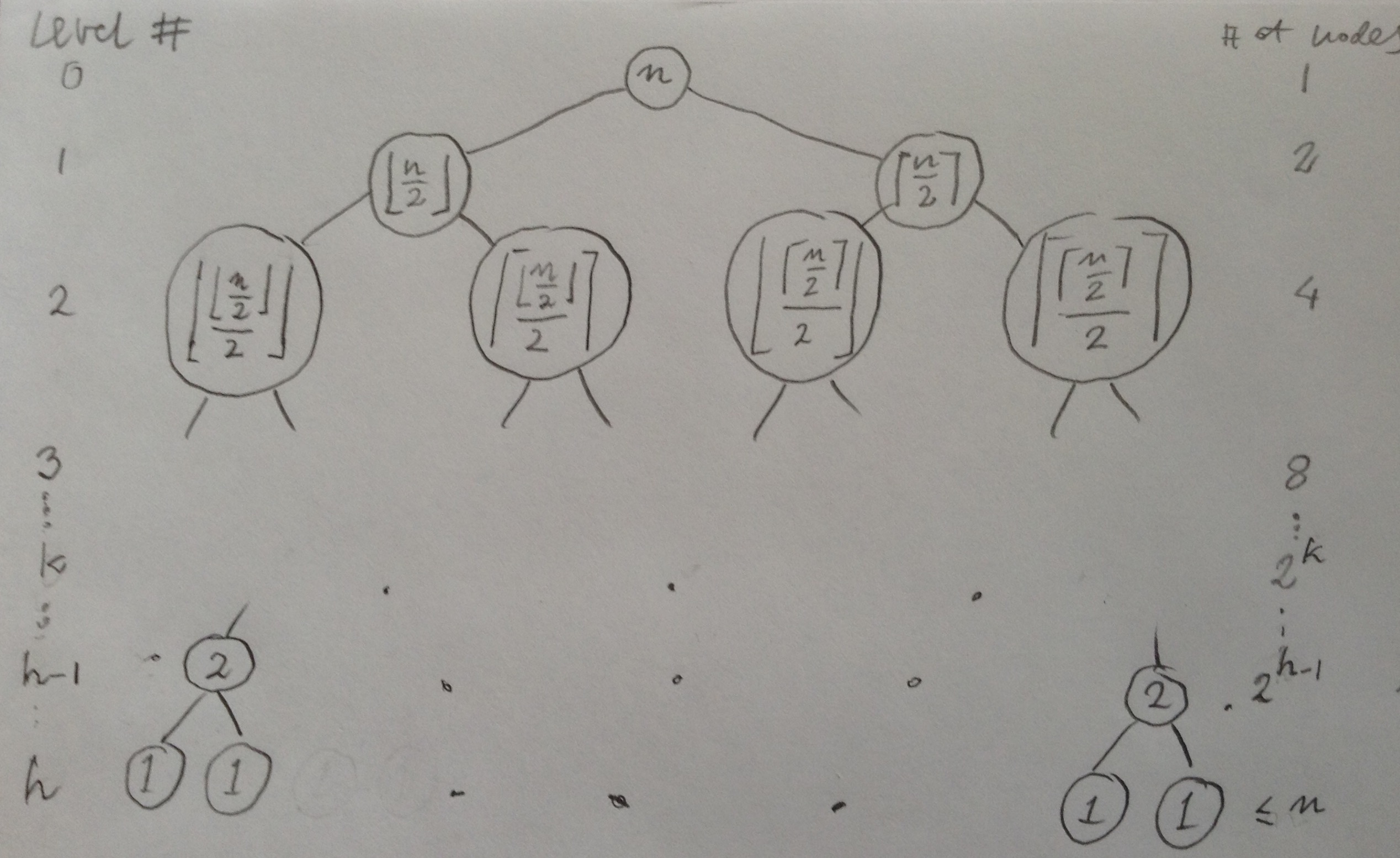
The obvious recursion tree for and sufficiently large is shown on Figure 2.
Figure 2: A sketch of the recursion 2-tree for for a sufficiently large , with levels shown on the left and the numbers of nodes shown on the right. The nodes correspond to calls to and show sizes of (sub)arrays passed to those calls. The last level is ; it only contains nodes with value 1. The root corresponds to the original call to . If a call that is represented by a node executes further recursive call to then these calls are represented by the children of ; otherwise is a leaf.
A recursive application of the equality333
It can be verified separately for odd and even values of .
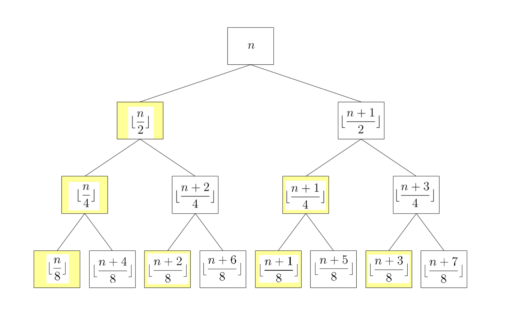
(1)
allows for rewriting of that tree onto one whose first four levels are shown on Figure 3.
Figure 3: The first four levels of the recursion 2-tree from Figure 2, with the equality (1) applied, recursively. The number of comparisons of keys performed in the best case by invoked in step 2c of Algorithm 2.1 as a result to a call to corresponding to a node of is equal to the number that is shown in its left child, highlighted yellow. All the right children at level of show numbers of the form , where . Thus all the left children (highlighted yellow) at level show numbers of the form , where .
2.2 Best-case and its characterization
The best-case arrays of sizes and for , where , are those in which every element of the first array is less than all elements of the second one. In such a case, performs of comps.
Thus the following recurrence relation for the least number of comparisons of keys that performs on any -element array is straightforward to derive from its description given by Algorithm 2.1.
(2)
and, for ,
(3)
Using the equality (1), the recurrence relation (3) is equivalent to:
Figure 4: Graph of the solution of the recurrence (2) and (3).
Unfolding the recurrence (4) allows for noticing that the minimum number of comps performed by all calls to is equal to the sum of all values shown at nodes highlighted yellow in the recursion tree of Figure 3. They may be summed-up level-by-level.
One can notice from Figure 3 that the number of comps performed at any level with the maximal number of nodes is given by this formula:
(5)
What is not clear is whether all levels of the recursion tree are maximal. Fortunately, the answer to this question does not depend on whether given instance of is running on a best-case array or on any other case of array. It has been known form a classic analysis of the worst-case running time of that every level of its recursion tree that contains at least one non-leaf, or - in other words - a node that shows value , is maximal. A page A contains a detailed derivation of that fact. Thus all levels 0 through of are maximal.
Therefore, the formula (5) gives the number of comps for every level .
The last level of may be not maximal because the level may contain leaves, or - in other words - nodes that show value , where for some , and as such do not have any children in level . However, for each such node the value of is 0, so it can be included in summation (5) without affecting its value even though the said value does not correspond to any node in level .
Therefore, the formula (5) gives the number of comps for level .
Also, the depth of is , as the Theorem A.0.2 page A.0.2 in A states.
Thus the minimum number of comps performed by is given by this formula:
(6)
Unfortunately, the summation (6) contains non-zero terms, so it cannot be evaluated quickly in its present form. Fortunately, its inner summation (5) can be reduced to a closed-form formula.
2.3 Zigzag function
In order to reduce (5) to a closed form, I am going to use function Zigzag defined by:
(7)
The following fact is instrumental for that purpose.
Theorem 2.2.
For every natural number n and every positive natural number m,
(8)
where Zigzag is a function defined by (7) and visualized on Figure 5.
Figure 5: Graph of function .
Proof.
The equality (8) can be verified experimentally, for instance, with a help of software for symbolic computation444
I used Wolfram Mathematica for that purpose.. The analytic proof is deferred to Section 7.
∎
Corollary 2.3.
For every natural number n and every positive natural number m,
(9)
where Zigzag is a function defined by (7) and visualized on Figure 5.
Proof.
First, let’s note555
Analytic proof of that fact is a straightforward exercise; see Appendix B page B. that
The following theorem yields the formula (13) for the minimum number of comps performed by .
Theorem 2.5.
For every natural number n,
(13)
where Zigzag is a function defined by (7) and visualized on Figure 5.
Proof.
∎
Figure 6: Graphs of functions (bottom line) and (top line) of equality (13). They coincide with each other for all natural numbers .
Formula (13), although not quite closed-form, comprises of summation with only closed-form terms, so it may be evaluated in time, where is a constant. I will show in Section 3 that (13) does not have a closed form.
Graphs of both sides of equality (13) are shown on Figure 6. Once can see that for natural numbers they coincide with the solution of recurrences (2) and (3) visualized on Figure 4.
Corollary 2.6.
For every natural number n, the minimum number of comps that performs while sorting an -element array is:
(14)
where Zigzag is a function defined by (7) and visualized on Figure 5.
3 A fractal in
A deceitfully simple expression
(15)
half of which occurs in formula (14) of Corollary 2.6, is a formidable adversary for those who may try to turn it into a closed form, although the time required for its evaluation for any given is 666
So, to all practical purposes, (14) is a closed-form formula.. That does not come as a surprise, taking into account that its graph, shown on Figure 7, bears a resemblance of fractal. This can be easily seen as soon as a sawtooth function is subtracted from it, yielding the function given by
(16)
Figure 7: A graph of function plotted against a sawtooth function .
Figure 8: A graph of function plotted below its tight linear upper bound (if can be shown that whenever
for some integer ); also shown below are the terms of the summation and their tight linear upper bound .
The function is a fractal with quasi similarity that repeats at intervals of exponentially growing length. It is a union
(19)
of functions , each having an interval as its domain. In other words, for every integer ,
Figure 9: A graph of the first six (the first one is ) normalized parts of function of Figure 8 plotted against the line . Also shown (in blue) are the first five terms , , of sums that occur in the formula (24) for ; for each integer and all ,
their parts above the -axis restricted to visualize a fragment of an infinite binary search trie defined as the set of shortest binary expansions of with the last digit (if the said binary expansion is finite) being interpreted as the sequence terminator; in particular, the root of is , and if is a finite binary sequence then the children of binary expansion are and .
Let be the normalized on interval , defined by:
(21)
and be the periodized by composing it with a sawtooth function ,777
The fractional part of . defined by:
(22)
Contracting definitions (20), (21), and (22), yields
(23)
One can compute888
An elementary geometric argument based on the graph visualized on Figure 9 will do. from (23) the following alternative formula for :
Since each function , and - therefore - each function , and - therefore - each function , are a result of smaller and smaller triangles piled, originating in function Zigzag of definition (18) of function , on one another as shown on Figure 9, for any integers , linearly interpolates . Because of that, each linearly interpolates the limit of all s defined by:
(25)
as Figure 10 illustrates.
An application of (24) to (25) yields:
(26)
Figure 10: Functions functions and their limit (the topmost curve) given by (26). Collapsing the Zigzag would yield the same, albeit scaled-down (by the factor of 2) pattern , as (26) does imply.
Since for every integer and , is integer, . Therefore, by virtue of (24) and (26), for every non-negative integer and ,
(27)
This and (24) eliminate the need for infinite summation999
As it appears in (26) while computing .
It can be shown that although a continuous function, is nowhere-differentiable. As such, it does not have a closed-form formula as any closed-form formula on a real interval must define a function have a derivative at every point of that interval, except for a non-dense set of its points. Since can be expressed in function, described by a closed-form formula, of the right-hand side of formula (13), the latter does not have a closed-form formula, either.
Theorem 3.1.
There is no closed-form formula the values of which coincide with for all positive integers , that is, for every closed-form formula on function Zigzag there is a positive such that
(28)
where Zigzag is a function defined by (7) and visualized on Figure 5.
Proof.
Follows from the above discussion. A more detailed proof is deferred to Section 8.
∎
This way I arrived at the following conclusion.
Corollary 3.2.
There is no closed-form formula for .
Proof.
A closed-form formula for would, by virtue of (14) page 14, yield a closed-form formula for , which by Theorem 3.1 does not exist.
∎
Note. One can apply the reverse transformations to those used in Section 3 on function and construct a fractal function , shown on Figure 11,
given by the equation
Figure 11: A graph of function plotted above a graph of the function
.
Computing values of function does not have to be as complex as (or more complex than) the definition (26) implies. Of course, for every integer , . One can apply some elementary arguments based on a structure visualized on Figure 10 to conclude that
(31)
(the latter being the maximum of ) or that for every positive integer ,
(32)
It takes a bit more work to compute
(33)
It turns out that computing values of function for every that has a finite binary expansion can be done easily if an oracle for computing the values of the function defined by (2) and (3) is given101010
Which is not that surprising after a glance at Figure 11.. Once that is accomplished, since is a continuous function and the set of numbers with finite binary expansions is dense in the set of reals, it allows for fast approximations of for every real . 111111
It helps to remember that is a periodic function with .
Theorem 4.1.
For every positive integer 121212Of course, one if free to assume that is odd here. and integer with ,
(34)
Proof.
The equality (34) can be verified experimentally, for instance, with a help of software for symbolic computation4. The analytic proof is deferred to Section 9.
∎
Theorem 4.1 allows for easy computing of if is given for some using this form of (34):
5 Relationship between the best case and the worst case
A casual student of tends to believe that its worst-case behavior is about twice as bad as its best-case behavior. This, of course, is only approximately true. In this Section, I will derive the exact difference between and using function defined by (16) page 16.
An exact formula for the number of comparisons of keys performed by in the worst case is known131313
See (75) in the A. and is given for any positive integer by the following equality:
For every positive integer , the difference between twice the number of comparison of keys performed in the best case and the number of comparison of keys performed in the worst case by while sorting an -element array is:
(see Figure 8 for explanation), I conclude with the following tight linear bounds on .
Corollary 5.2.
For every positive integer , the difference between twice the minimum number and the maximum number of comparison of keys performed in the worst case by while sorting an -element array satisfies this inequality:
Figure 12: A graph of shown between graphs of its tight linear bounds and .
Obviously, whenever , that is, whenever . It can be shown that whenever
for some integer .
A graph of and its tight bounds are shown on Figure 12.
6 The sum of digits problem
A known explicit formula, published in [7], for the total number
of bits in all integers between 0 and (not including 0 and ) is expressed in terms of function Zigzag (referred to as in [7]) and is given by:141414
The following are screen shots and an excerpt from [7].
Let be periodic of period 1 and defined on by
It has been shown in [3] that the recurrence relation for is the same as the recurrence relation for given by (2) and (3). Therefore, the formula (13) derived in this paper is equivalent to given above by the considerably more complicated definition.
Interestingly, the above definition can be simplified to (13) along the lines of the elementary derivation of the alternative formula (36) for on page 36151515
Even more interestingly, if someone did bother to simplify Trollope’s formula of [7] then I am not aware of it..
In this Section, I provide an analytic proof of the experimentally-derived Theorem 2.2 page 2.2, Subsection 2.3 that was instrumental for the derivation of a logarithmic-length formula161616
, where . for . The result
and its proof have a flavor of Concrete Mathematics. Although they are interesting in their own right, they cannot be found in [4].
Theorem 7.1.
(Same as Theorem 2.2.)
For every natural number n and every positive natural number m,
(41)
where Zigzag is a function defined by (7) and visualized on Figure 5 page 5.
In this Section, I present a brief discussion/motivation of what can be generally considered a closed-form formula for a function from the set of real numbers into a set of real numbers. I provide an analytic proof of Theorem 3.1 page 3.1, Section 3 that implies the non-existence of closed-form formula for the minimum number of comparisons of keys by while sorting an -element array. I am going to use the acronym as an abbreviation for closed-form formula.
For reader’s convenience, the Theorem 3.1 is quoted below as Theorem 8.1.
Theorem 8.1.
(Same as Theorem 3.1.)
There is no the values of which coincide with
for all positive integers , that is, for every on function Zigzag there is a positive such that
(49)
where Zigzag is a function defined by (7) and visualized on Figure 5.
The rest of this Section constitutes the proof of Theorem 8.1.
First, let me use an example of function as an insight of what may be accepted as a for a continuous function - like, say, - on the set of reals or on an interval thereof. One picks a dense171717
In the metric topology of . subset of , with a collection of mappings , where , given by so that . Since for any , has been defined as
(50)
is considered a for .
Lemma 8.2.
For every positive integer ,
(51)
where the function has been defined by the equality (16) page 16,
the function , visualized on Figure 13181818Also, together with its partial sums, on Figure 10, page 10., has been defined by the equality (26) page 26, and the function has been defined by the equations (2) and (4) page 2.
If the function defined by the equations (2) and (4) has a then the function defined by the equation (26) page 26 has a .
Proof.
Let
(56)
be the set of rationals in the interval with finite binary expansions191919
It is a trivial exercise to show that every real number with finite binary expansion in the interval is of the form for some , and it is obvious that every real number of that form has a finite binary expansion and falls into that interval., enumerated by given by and visualized on Figure 14.
Figure 14: A graph of enumeration of the set .
is a dense subset of the interval of reals. Indeed, if then for every , and
(57)
Hence, for any , putting
(58)
so that
[the last equality holds because so that and ],
or
Should the nowhere-differentiable function have a , it would be differentiable everywhere except, perhaps, on a non-dense subset of . The following inductive argument demonstrates that. All atomic s are differentiable except, perhaps, on a non-dense subset of . If a finite number of s are differentiable except, perhaps, on non-dense subsets of then their composition is differentiable except, perhaps, on non-dense subsets of . 202020
For instance, function is differentiable on , except for the non-dense set . Thus has no .
The above observation, together with Lemma 8.3, complete the proof of Theorem 8.1.
In this Section, I provide an analytic proof of experimentally-derived Theorem 4.1 page 4.1, Section 4. This result, re-stated by Theorem 9.1 below, allows for practically efficient computations of values of the continuous Blackmange function for reals with finite binary floating-point representations. I also provide some properties (Lammas 9.2, 9.3, and 9.4) of the Zigzag function, given by the equality (7) page 7 and visualized on Figure 5 page 5, that are useful for a neat derivation of a formula for the Blancmange function as (the limit of) a finite sum of some values of the Zigzag function.
Let the function212121
Known as the Blancmange function.
, visualized on Figure 13 page 13, be defined by
(26) page 26, and , given by (2) and (4) page 2, be the least number of comparisons of keys that performs while sorting an -element array.
Theorem 9.1.
(Same as Theorem 4.1.)
For every positive integer 222222Of course, one if free to assume that is odd here. and integer with ,
(61)
The reminder of this Section constitutes a proof of Theorem 9.1.
Note. Function Zigzag, visualized on Figure 5 page 5, has been defined by (7) page 7.
Note. A glance at the proof of Lemma 9.3 suffices to notice that it fails if , and so does Theorem 4.1. In particular, for , Lemma 8.2 page 8.2 yields
(68)
since for ,
References
[1]
Sara Baase.
Computer Algorithms: Introduction to Design and Analysis.
Addison-Wesley Publishing, 2nd edition, 1991.
[2]
Donald E. Knuth.
The Art of Computer Programming, volume 3.
Addison-Wesley Publishing, 2nd edition, 1997.
[3]
M. D. McIlroy.
The number of 1’s in binary integers: Bounds and extremal
properties.
SIAM Journal of Computing, 3(4):255–261, December 1974.
[4]
Donald Knuth Ronald Graham and Oren Patashnik.
Concrete Mathematics: A Foundation for Computer Science.
Addison–Wesley, 1994.
[5]
Robert Sedgewick and Philippe Flajolet.
An Introduction to the Analysis of Algorithms.
Pearson, 2013.
[6]
Marek A. Suchenek.
Best-case analysis of MergeSort with an application to the sum of
digits problem (MS).
https://arxiv.org/pdf/1607.04604v1, July 18 2016.
[7]
J. R. Trollope.
An explicit expression for binary digital sums.
Mathematics Magazine, 41(1):21–25, Jan.–Feb. 1968.
APPENDIX
Appendix A A derivation of the worst-case running time of
Let’s assume that is large enough to spur a cascade of many recursive calls to following the recursion tree , a sketch of which
is shown on Figure 2.
The nodes in tree correspond to calls to and show sizes of (sub)arrays passed to those calls. The root corresponds to the original call to . If a call that is represented by a node executes further recursive calls to then these calls are represented by the children of ; otherwise is a leaf. Thus, is a -tree232323
A binary tree whose every non-leaf has exactly children..
The levels in tree are enumerated from to , where is the number of the last level of the tree, or - in other words - the depth of . On Figure 2, they are shown on the left side of the tree. The root is at the level , its children are at level , its grand children are at level , its great grand children (not shown on the sketch) are at level , at so on.
Clearly, since every call to on a sub-array of size executes two further recursive calls to , only the nodes that show value are leaves and all other nodes have children each. Thus, since all nodes in the last level are leaves, they all show value . And since the original input array gets split, eventually, onto -element sub-arrays, the number of all leaves in is . (This, however, does not mean that the last level necessarily contains all the leaves of .)
If a level has nodes, each of them showing a value , then each such node has children so that level has twice the number of nodes in level , that is, nodes. Since level has nodes, it follows (completion of a proof by induction with the basis and inductive steps outlined above is left as an exercise for the reader) that if is the level number of any level above which all the nodes show values then all levels contain exactly nodes each.
The last level may contain nodes or less. We are going to show that each level above level contains exactly nodes. Here is a very insightful property that we are going to use for that purpose. It states that is splitting its input array fairly evenly so that at any level of the recursive tree, the difference between the lengths of the longest sub-array and the shortest sub-array is This fact is the root cause of
good worst-case performance
of .
Property A.0.1.
The difference between values shown by any two nodes in the same level of the recursion tree for is .
Proof.
The Property clearly holds for level . We will show that if it holds for level and is not the last level of the recursion tree (that is, ) then it also holds for the level .
Let us assume that the Property holds for some level .
Let be numbers shown by any two (not necessarily distinct) nodes in level . It suffices to show that
(69)
Let be the numbers shown by the parents of the mentioned above nodes. Those parents, of course, must reside in the level . By the inductive hypothesis (that holds for level ), , that is,
(70)
The numbers shown by all their four children are , , and , respectively, so the largest difference between any of those four numbers is . In particular, is not larger than that.
We have:
Thus (69) holds.
This completes the inductive step and completes the proof of the Property.
∎
As we have noted, the values shown at all nodes in the last level are all . Thus the values shown at their parents, that reside at level are all , and the values shown at their grand parents, that reside at level are all . Thus, by Property A.0.1, all nodes at level show values , and, therefore (as we have proved before), all levels have nodes, each, as it has been visualized on Figure 2.
Theorem A.0.2.
The depth of the recursion tree for
run on an array of size is
(71)
Proof.
Since every level of , except, perhaps, for the last level, has the maximal number of nodes, a 2-tree with leaves could not be any shorter than . So, is a shortest 2-tree with leaves. Therefore (by a well known fact), its depth is equal to . Thus (71) holds.
∎
Because each node in any level above shows value , it has children. Thus the value it shows is equal to the sum of values shown by its children, as we have indicated at the beginning of this section. From that we conclude (a proof by induction is left as an exercise for the reader) that the sum of values shown at nodes in any level is the same for each such level. Thus the said sum is equal to the value showed by the only node at level 0, that is, is equal to .
Let be the values shown at the nodes of some level . The number of comps performed by a call to invoked by the call to on an array of elements is either if (no call to is made) or, as we have shown in the previous section, is if . So, in either case, it is .
Thus the number of comps performed at level is
(72)
Moreover, since all nodes at the last level are 1’s
(73)
Therefore, the total number of comps that performs in the worst case on an -element array is equal to
The number of comparisons of keys that performs in the worst case while sorting an -element array is
(74)
Proof follows from the above derivation.
Using the well-known242424
See [2]. closed-form formula for ,
I conclude that
(75)
Appendix B Proof of
Theorem B.0.1.
For every natural number n and every positive natural number m,
Proof.
Let , where .
We have
Therefore,
∎
References
[1]
Sara Baase.
Computer Algorithms: Introduction to Design and Analysis.
Addison-Wesley Publishing, 2nd edition, 1991.
[2]
Donald E. Knuth.
The Art of Computer Programming, volume 3.
Addison-Wesley Publishing, 2nd edition, 1997.
[3]
M. D. McIlroy.
The number of 1’s in binary integers: Bounds and extremal
properties.
SIAM Journal of Computing, 3(4):255–261, December 1974.
[4]
Donald Knuth Ronald Graham and Oren Patashnik.
Concrete Mathematics: A Foundation for Computer Science.
Addison–Wesley, 1994.
[5]
Robert Sedgewick and Philippe Flajolet.
An Introduction to the Analysis of Algorithms.
Pearson, 2013.
[6]
Marek A. Suchenek.
Best-case analysis of MergeSort with an application to the sum of
digits problem (MS).
https://arxiv.org/pdf/1607.04604v1, July 18 2016.
[7]
J. R. Trollope.
An explicit expression for binary digital sums.
Mathematics Magazine, 41(1):21–25, Jan.–Feb. 1968.


![[Uncaptioned image]](1607.04604v2/Quote_from_Trollope_A.png)
![[Uncaptioned image]](1607.04604v2/Quote_from_Trollope.png)