Black Box Linear Algebra: Extending Wiedemann’s Analysis of a Sparse Matrix Preconditioner for Computations over Small Fields

Wayne Eberly Affiliation: Department of Computer Science Affiliation: University of Calgary

Abstract

Wiedemann’s paper, introducing his algorithm for sparse and structured matrix computations over arbitrary fields, also presented a pair of matrix preconditioners for computations over small fields. The analysis of the second of these is extended in order to provide more explicit statements of the expected number of nonzero entries in the matrices obtained as well as bounds on the probability that such matrices have maximal rank.

This is part of ongoing work to establish that this matrix preconditioner can also be used to bound the number of nontrivial nilpotent blocks in the Jordan normal form of a preconditioned matrix, in such a way that one can also sample uniformly from the null space of the originally given matrix. If successful this will result in a black box algorithm for the type of matrix computation required when using the number field sieve for integer factorization that is provably reliable and — by a small factor — asymptotically more efficient than alternative techniques that make use of other matrix preconditioners or require computations over field extensions.

1 Introduction

Suppose that $\textup{{F}}=\textup{{F}}_{q}$ is a finite field with size $q$ . Let $m$ and $n$ be integers such that $0\leq m\leq n$ . The paper that introduced Wiedemann’s algorithm [2] also includes a proof of the following claim — which concerns an $n\times n$ matrix obtained by appending an additional set of row vectors to a matrix $A\in\textup{{F}}^{m\times n}$ with maximal rank:¹¹ 1 Wiedemann attributes much of the proof of this claim to an anonymous referee who is thanked for allowing this work to be included.

Theorem $\text{{1}}^{\prime}$ [Wiedemann]: Numbers $\epsilon>0$ and $c_{1}$ exist, both independent of $q$ , with the following property: For any integers $n>m\geq 0$ a random procedure exists for generating $n-m$ row vectors with length $n$ such that if $A$ is an $m\times n$ matrix of rank $m$ , then with probability at least $\epsilon$ , the resulting $n\times n$ matrix is nonsingular and the total Hamming weight of the generated rows is at most $1+c_{1}n\log n$ .

Unfortunately the unknown constants $\epsilon$ and $c_{1}$ are neither supplied nor estimated. Furthermore, it seems that if the proof in [2] is applied without change in order to determine these values then either $c_{1}$ must be so large or $\epsilon$ so tiny that the result is of limited practical interest.

This is, somewhat, rectified in Section 2: While the outline of Wiedemann’s argument is maintained, along with the details of several steps, several other components are revised or replaced entirely in order to remove unnecessary bounds on various parameters and to simplify the estimation of the unknown parameters $\epsilon$ and $c_{1}$ . The bound $\epsilon$ is also increased by adding another $\ell$ rows to the resulting matrix $B\in\textup{{F}}^{(n+\ell)\times n}$ rows; here, $\ell$ depends on the size of the field F. In particular, the following result is obtained.

Theorem 1.1.

Let $\textup{{F}}=\textup{{F}}_{q}$ be the finite field with size $q$ . Let $m$ and $n$ be integers such that $n\geq m\geq 0$ . Let $\ell$ be a nonnegative integer and let $\sigma$ , $\tau$ and $\upsilon$ be positive constants (depending on $q$ , but independent of $n$ and $m$ ) as given in Table 1 on page 1.

A random procedure exists for generating $n-m+\ell$ rows with length $n$ such that if $A$ is an $m\times n$ matrix of rank $m$ , then an additional $m+\ell$ rows (each with length $n$ ) are produced, and the expected number of nonzero entries in these rows is $\sigma n\ln n+\tau n$ if $n-m\geq\upsilon$ , and at most $\frac{q-1}{q}(n-m+\ell)n\leq\frac{q-1}{q}(\upsilon+\ell)n$ , otherwise.

If $q\leq n^{2}$ then the matrix $B\in\textup{{F}}^{(n+\ell)\times n}$ obtained from $A$ by adding these rows has maximal rank $n$ with probability at least $\frac{9}{10}$ . If $q>n^{2}$ then this matrix has maximal rank with probability at least $\frac{9}{10}-\frac{9}{10n}$ .

The probability bounds listed above are quite arbitrary. The parameter $\sigma$ does not depend on this probability. Formulas for $\ell$ , $\tau$ and $\upsilon$ , depending on the field size $q$ and an arbitrarily small failure probability $\epsilon$ , are given in Section 2.

$q$	$\ell$	$\sigma$	$\tau$	$\upsilon$	$q$	$\ell$	$\sigma$	$\tau$	$\upsilon$
$2$	$8$	$\frac{43}{2}$	$17$	$41$	$13$	$3$	$\frac{120}{13}$	$6$	$150$
$3$	$5$	$16$	$11$	$55$	$16$ – $19$	$2$	$\frac{9(q-1)}{q}$	$5$	$194$
$4$	$4$	$\frac{225}{16}$	$9$	$65$	$23$ – $29$	$2$	$\frac{8(q-1)}{q}$	$4$	$285$
$5$	$4$	$\frac{64}{5}$	$8$	$75$	$31$ – $43$	$2$	$\frac{15(q-1)}{2q}$	$4$	$381$
$7$	$3$	$\frac{78}{7}$	$7$	$96$	$47$ — $59$	$2$	$\frac{7(q-1)}{q}$	$4$	$577$
$8$	$3$	$\frac{21}{2}$	$6$	$108$	$61$ – $71$	$2$	$\frac{27(q-1)}{4q}$	$4$	$783$
$9$	$3$	$\frac{88}{9}$	$6$	$124$	$73$ – $83$	$2$	$\frac{33(q-1)}{5q}n$	$4$	$996$
$11$	$3$	$\frac{105}{11}$	$6$	$136$	$\geq 89$	$2$	$\frac{13(q-1)}{2q}$	$4$	$1213$

Figure 1: Bounds Established in Section 2

A second result, which is also proved in Section 2, establishes that the constant $\sigma$ , mentioned above, can be made arbitrarily close to $6\left(1-\frac{1}{q}\right)$ , provided that the minimum field size $q$ and the constant $\upsilon$ are both increased — at the cost of increasing the constants $\ell$ , $\tau$ and $\upsilon$ (but not $\sigma$ ) that are listed.

Theorem 1.2.

Let $N$ be an integer such that $N\geq 18$ . Let $\textup{{F}}_{q}$ be a finite field with size $q\geq 16N+9$ Let $m$ and $n$ be integers such that $n\geq m\geq 0$ . Let $\sigma=\left(1-\frac{1}{q}\right)\ \cdot\left(6+\frac{3}{N}\right)$ , $\tau=1$ , and $\upsilon=\lceil(2N+1)\ln(2N+1)+\frac{167}{5}(2N+1)\rceil$ .

A random procedure exists for generating $n-m$ rows with length $n$ such that if $A$ is an $m\times n$ matrix of rank $m$ , then an additional $m$ rows (each with length $n$ ) are produced, and the expected number of nonzero entries in this row is $\sigma n\ln n+\tau n$ if $n-m\geq\upsilon$ , and at most $\frac{q-1}{q}(n-m)n\leq\frac{q-1}{q}\upsilon n$ , otherwise.

If $q\leq n^{2}$ then the matrix $B\in\textup{{F}}^{n\times n}$ obtained from $A$ by adding these rows is nonsingular with probability at least $\frac{8}{9}$ . If $q>n^{2}$ then this matrix is nonsingular with probability at least $\frac{8}{9}-\frac{8}{9n}$ .

Once again, the probability bounds here are quite arbitrary, and probability bounds that are closer to one can be obtained by applications of the same techniques, at the cost of increasing the values of the constants $\tau$ and $\upsilon$ .

This is work in progress. Future versions of this report will document progress in establishing that this yields an efficient matrix preconditioner, to bound the number of nontrivial nilpotent blocks of a conditioned matrix without lowering matrix rank, for matrices over small finite fields.

2 A Modified Proof of Wiedemann’s Result

This section describes modifications to Wiedemann’s argument needed to establish Theorems 1.1 and 1.2.

2.1 Getting Started — and Improving Reliability by Adding Rows

Suppose that $m$ and $n$ are positive integers such that $0\leq m\leq n$ and $A\in\textup{{F}}^{m\times n}$ is a matrix with maximal rank $m$ , where $\textup{{F}}=\textup{{F}}_{q}$ is a finite field with size $q$ . Following Wiedemann’s argument, let us begin by assuming that $q\leq n^{2}$ and suppose, as well, that

n=m+k+c_{2}

(2.1)

where $c_{2}$ will be defined later.

Suppose first that $k\leq c_{3}\ln n$ , where $c_{3}$ is another constant to be chosen later, and that the remaining $n-m+\ell$ rows of an $(n+\ell)\times n$ matrix $B$ are chosen uniformly and independently from $\textup{{F}}^{1\times n}$ . The following lemma, which is easily proved, bounds the probability that the rank of $B$ is less than $n$ in this case.

Lemma 2.1.

Let $\ell$ be a nonnegative integer and let $B\in\textup{{F}}^{(n+\ell)\times n}$ be a matrix produced by appending another $n-m+\ell$ rows, selected uniformly and independently from $\textup{{F}}^{1\times n}$ , to $A$ . Then the probability that the rank of $B$ is less than $n$ is at most $q^{-\ell}$ .

Furthermore, if $q\geq 3$ then the top $n\times n$ submatrix of $B$ is nonsingular with probability at least $\frac{1}{q-1}$ .

Proof.

Permuting the columns of $A$ (and $B$ ) as needed we may assume without loss of generality that the principal $m\times m$ submatrix of $A$ is nonsingular. Let us continue by choosing the entries in the leftmost $m$ columns of the $n-m+\ell$ rows that are to be appended to $A$ . Regardless of the choice of these entries, this completes an $(n+\ell)\times m$ submatrix of $B$ , including the leftmost $m$ columns, that must also have maximal rank $m$ .

The remaining entries of the top $m$ rows of $B$ are, of course, fixed: They are entries of $A$ . The entries in the lower columns may now be chosen freely and (viewing the selection of these entries in column order, instead of row order) a standard argument establishes that, for $1\leq i\leq n-m$ , if the leftmost $m+i-1$ columns of $B$ are linearly independent then the probability that the $m+i^{\text{th}}$ column of $B$ is a linear combination of these columns is at most $q^{m+i-n-\ell-1}$ . It now follows that $B$ has rank less than $n$ with probability at most

\sum_{i=1}^{n-m}q^{m+i-n-\ell-1}<\sum_{j\geq 0}q^{-(\ell+1)-j}=\frac{q^{-(\ell+1)}}{1-q^{-1}}\leq q^{-\ell}.

Finally, if $q\geq 3$ then, setting $\ell=0$ , one can see the (top) $n\times n$ submatrix obtained by appending these rows is singular with probability at most $\frac{q^{-1}}{1-q^{-1}}=\frac{1}{q-1}$ , as claimed. ∎

Since $n-m=k+c_{2}$ , the expected number of nonzero entries in these rows is

\left(\frac{q-1}{q}\right)(k+c_{2}+\ell)n<\left(\frac{q-1}{q}\right)\cdot\left(c_{3}n\ln n+(c_{2}+\ell)n\right)

when $k\leq c_{3}\ln n$ .

With that noted let us suppose, instead, that $k>c_{3}\ln n$ . Following Wiedemann once again, let

z=1-\frac{c_{3}\ln n}{k}>0.

(2.2)

Suppose that, for the initial $k$ rows, each entry is set to zero with probability $z$ . The remaining unset entries are then chosen uniformly and independently from F. The expected number of nonzero entries in these rows is then

\left(\frac{q-1}{q}\right)c_{3}n\ln n.

If the entries of another $c_{2}+\ell$ rows are chosen uniformly and independently from F then the expected number of nonzero entries in these rows is

\left(\frac{q-1}{q}\right)(c_{2}+\ell)n.

Consequently the expected number of nonzero entries in all these rows is less than

\left(\frac{q-1}{q}\right)\cdot\left(c_{3}n\ln n+(c_{2}+\ell)n\right)

in this case as well.

The bulk of the rest of Wiedemann’s argument concerns the derivation of an upper bound for the probability that $B$ has rank less than $n$ if $k>c_{3}\ln n$ and the rows of $B$ are chosen in this way.

Following Wiedemann, let $\rho$ be the probability that the rows of $A$ , together with the first $k$ (sparse) rows generated using the above process, are linearly dependent — that is, the probability that the space spanned by these vectors has dimension less than $m+k$ . Wiedemann shows that

\rho\leq\rho_{0}+\rho_{1}

(2.3)

where

\rho_{0}=\sum_{1\leq j\leq k\beta_{0}}\binom{k}{j}(q-1)^{j}\left(q^{-1}+\frac{(q-1)}{q}(nq)^{-c_{4}\beta}\right)^{n-m},

(2.4)

and

\rho_{1}=\sum_{k\beta_{0}<j\leq k}\binom{k}{j}(q-1)^{j}\left(q^{-1}+\frac{(q-1)}{q}(nq)^{-c_{4}\beta}\right)^{n-m},

(2.5)

when

c_{4}=\frac{c_{3}}{3},

(2.6)

and when

\beta=\frac{j}{k}

(2.7)

in the above expressions, and where $\beta_{0}$ is yet another constant to be defined later.

A useful bound for $\rho_{1}$ is next obtained: Assuming that

c_{2}\geq\frac{3}{2}\geq\log_{2}e\qquad\text{and}\qquad c_{4}\geq\frac{2}{\beta_{0}},

(2.8)

Wiedemann establishes that

\rho_{1}\leq 2q^{-c_{2}}.

(2.9)

Wiedemann continues by observing that

\rho_{0}\leq\sum_{1\leq j<k\beta_{0}}\left(\frac{1}{\beta^{\beta}(1-\beta)^{1-\beta}}f(q)\right)^{k},

(2.10)

where

f(x)=(x-1)^{\beta}\left(x^{-1}+(1-x^{-1})(nx)^{-c_{4}\beta}\right).

(2.11)

2.2 Getting to the Next Step by a Different Route

Wiedemann continues by using the above to establish that

\rho_{0}\leq\sum_{1\leq j<k\beta_{0}}\beta^{k\beta}.

(2.12)

Unfortunately, Wiedemann’s involves a Taylor series approximation that seems only to be accurate for a limited range of values, and might suggest that either $\beta$ must be tiny or $c_{4}$ must be huge in order for it to be applicable. The argument that follows is, therefore, quite different from given by Wiedemann [2].

With that noted, consider the equation at lines (2.10) and (2.11) once again. These imply that

\begin{split}\rho_{0}&\leq\sum_{1\leq j<k\beta_{0}}\left(\frac{(q-1)^{\beta}}{\beta^{\beta}(1-\beta)^{1-\beta}}\left(\frac{1}{q}+\frac{q-1}{q}(nq)^{-c_{4}\beta}\right)\right)^{k}\\ &\leq\sum_{1\leq j<k\beta_{0}}\left(\frac{(q-1)^{\beta}}{\beta^{\beta}(1-\beta)^{1-\beta}}\left(\frac{1}{q}+\frac{q-1}{q}\left(\frac{\beta}{q}\right)^{c_{4}\beta}\right)\right)^{k}\end{split}

(2.13)

since $n^{-1}\leq k^{-1}\leq\frac{j}{k}=\beta$ . It follows from this that

\rho_{0}<\sum_{1\leq j<k\beta_{0}}\left(\frac{1}{\beta^{\beta}(1-\beta)^{1-\beta}}\left(\frac{(q-1)^{\beta}}{q}+\frac{(q-1)q^{(1-c_{4})\beta}}{q}\beta^{c_{4}\beta}\right)\right)^{k}.

(2.14)

2.2.1 Bounding Terms in $\boldsymbol{\rho_{0}}$ When $\boldsymbol{\beta}$ is Extremely Small

Note that $\displaystyle{\lim_{\beta\rightarrow 0^{+}}}\beta^{\beta}=\displaystyle{\lim_{\beta\rightarrow 0^{+}}}(1-\beta)^{1-\beta}=1$ , and $\beta^{\beta}<1$ when $0<\beta<1$ . The bounds given at lines (2.13) and (2.14) can be simplified by establishing a lemma like the following, allowing the factor $(1-\beta)^{-(1-\beta)}$ to be replaced by a factor $\beta^{\gamma\beta}$ , for a negative constant $\gamma$ , when $\beta$ is small.

Lemma 2.2.

Consider the relationship between $(1-x)^{-(1-x)}$ and $x^{\gamma x}$ , for a negative constant $\gamma$ , when $x$ is small and positive.

(a)

If $0<x\leq\frac{5}{43}$ then $(1-x)^{-(1-x)}\leq x^{\gamma x}$ , with $\gamma=-\frac{11}{25}$ .
(b)

If $0<x\leq\frac{1}{5}$ then $(1-x)^{-(1-x)}\leq x^{\gamma x}$ , with $\gamma=-\frac{23}{40}$ .

Proof.

Consider the function

g(x)=\gamma x\ln x+(1-x)\ln(1-x)

when $\gamma$ is a negative constant and $0<x<1$ . Since $e^{g(x)}=\frac{x^{\gamma x}}{(1-x)^{-(1-x)}}$ and $(1-x)^{-(1-x)}>0$ , $(1-x)^{-(1-x)}\leq x^{\gamma x}$ (for $0<x<1$ ) if and only if $g(x)\geq 0$ .

Now

$\displaystyle\lim_{x\rightarrow 0^{+}}g(x)$	$\displaystyle=\lim_{x\rightarrow 0^{+}}\frac{\gamma\ln x}{x^{-1}}+\lim_{x\rightarrow 0^{+}}(1-x)\ln(1-x)$
	$\displaystyle=\lim_{x\rightarrow 0^{+}}\frac{\gamma\ln x}{x^{-1}}$
	$\displaystyle=\lim_{x\rightarrow 0^{+}}\frac{\gamma x^{-1}}{-x^{-2}}$	(by l’Hôpital’s Rule)
	$\displaystyle=\lim_{x\rightarrow 0^{+}}-\gamma x=0.$

It is easily checked that $g^{\prime}(x)=\gamma\ln x-\ln(1-x)+\gamma-1$ . Thus $\displaystyle{\lim_{x\rightarrow{0^{+}}}}g^{\prime}(x)=+\infty$ , so that $g^{\prime}(x)>0$ when $x$ is small and positive. It follows from the above that $g(x)>0$ when $x$ is small and positive, as well.

Note next that $g^{\prime\prime}(x)=\frac{\gamma}{x}+\frac{1}{1-x}$ , so that $\displaystyle{\lim_{x\rightarrow 0^{+}}}g^{\prime\prime}(x)=-\infty$ , since $\gamma<0$ , and $g^{\prime\prime}(x)<0$ when $x$ is small and positive. On the other hand, $g^{\prime\prime\prime}(x)=-\frac{\gamma}{x^{2}}+\frac{1}{(1-x)^{2}}>0$ when $0<x<1$ .

It now follows that $g(x)\geq 0$ for $0<x\leq\delta$ if $g(\delta)\geq 0$ and $g^{\prime}(\delta)<0$ : Since $g^{\prime\prime\prime}(x)>0$ for all $x$ such that $0<x<1$ , this implies that either

i.

$g(x)\geq 0$ for all $x$ such that $0<x<1$ ,
ii.

there exists a value $\Gamma$ such that $0<\Gamma<1$ , $g^{\prime}(x)\geq 0$ when $0<x\leq\Gamma$ and $g^{\prime}(x)<0$ when $\Gamma<x<1$ , or
iii.

there exist values $\Gamma_{1}$ and $\Gamma_{2}$ such that $0<\Gamma_{1}<\Gamma_{2}<1$ , $g^{\prime}(x)\geq 0$ when $0<x\leq\Gamma_{1}$ , $g^{\prime}(x)\leq 0$ when $\Gamma_{1}\leq x\leq\Gamma_{2}$ , and $g^{\prime}(x)>0$ when $\Gamma_{2}<x<1$ .

The claim is certainly trivial in the first case. In the second case it necessarily follows that $\Gamma<\delta$ , while it follows that $\Gamma_{1}<\delta<\Gamma_{2}$ in the third case. In each of the last two cases, the function $g$ is either nondecreasing or has a local maximum in the interval $0<x\leq\delta$ . In either case, it is minimized at one or the other of this interval’s endpoints. Since $\displaystyle{\lim_{x\rightarrow 0^{+}}}g(x)=0$ , it therefore suffices to confirm that $g(\delta)\geq 0$ in order to establish that $g(x)\geq 0$ when $0<x\leq\delta$ .

Part (a) of the claim can now be established by choosing $\gamma=-\frac{11}{25}$ and $\delta=\frac{5}{43}$ ; then $g^{\prime}(\delta)=-\frac{11}{25}\ln\frac{5}{43}-\ln\frac{38}{43}-\frac{36}{25}<-0.3<0$ and $g(\delta)=-\frac{11}{215}\ln\frac{5}{43}+\frac{38}{43}\ln\frac{38}{43}>0.0008>0$ , as required.

Part (b) of the claim can be established by choosing $\gamma=-\frac{23}{40}$ and $\delta=\frac{1}{5}$ ; then $g^{\prime}(\delta)=\frac{23}{40}\ln 5-\ln\frac{4}{5}-\frac{63}{40}<-0.4<0$ and $g(\delta)=\frac{23}{200}\ln 5+\frac{4}{5}\ln\frac{4}{5}>0.006>0$ . ∎

Suppose, now, that $\gamma\in\mathbb{Q}$ is a negative constant such that $(1-\beta)^{-(1-\beta)}\leq\beta^{\gamma\beta}$ when $0<\beta\leq\Delta$ for a positive constant $\Delta$ ; it follows by the above lemma that one might choose $\gamma=-\frac{11}{25}$ if $\Delta=\frac{5}{43}$ , and that one might choose $\gamma=-\frac{23}{40}$ if $\Delta=\frac{1}{5}$ . It would follow from the inequality at line (2.14) that

\rho_{0}\leq\sum_{1\leq j<k\beta_{0}}\left(\beta^{(\gamma-1)\beta}\left(\frac{(q-1)^{\beta}}{q}+\frac{(q-1)q^{(1-c_{4})\beta}}{q}\beta^{c_{4}\beta}\right)\right)^{k}

(2.15)

This can be further simplified by bounding $(q-1)^{\beta}$ by $\beta^{\delta\beta}$ for a small positive constant $\delta$ :

Lemma 2.3.

Consider the relationship between $\zeta^{x}$ and $x^{\delta x}$ when $\zeta$ is a positive constant.

If $\zeta=2$ and $0<x\leq\frac{1}{5}$ then $\zeta^{x}\leq x^{\delta x}$ when $\delta=-\frac{9}{20}$ .

Proof.

Consider the function

h(x)=\delta x\ln x-x\ln\zeta

when $\delta$ is a negative constant and $\zeta$ is a positive one. Since $e^{h(x)}=\frac{x^{\delta x}}{\zeta^{x}}$ and $\zeta^{x}>0$ when $x>0$ , $\zeta^{x}\leq x^{\delta x}$ (for positive $x$ ) if and only if $h(x)\geq 0$ .

Now note that

$\displaystyle\lim_{y\rightarrow 0^{+}}h(y)$	$\displaystyle=\lim_{y\rightarrow 0^{+}}\frac{\delta\ln y}{y^{-1}}-0$
	$\displaystyle=\lim_{y\rightarrow 0^{+}}\frac{\delta y^{-1}}{-y^{-2}}$	(by l’Hôpital’s Rule)
	$\displaystyle=\lim_{y\rightarrow 0^{+}}-\delta y=0.$

It is easily checked that $h^{\prime}(x)=\delta\ln x+\delta-\ln\zeta$ . Now $\displaystyle{\lim_{y\rightarrow 0^{+}}}h^{\prime}(y)=+\infty$ , since $\delta<0$ , so that $h^{\prime}(x)>0$ for sufficiently small positive $x$ . It follows by the above that $h(x)>0$ when $x$ is small and positive as well.

Since $h^{\prime\prime}(x)=\frac{\delta}{x}<0$ when $x>0$ it now follows, for any positive constant $\rho$ , that if $h(\rho)\geq 0$ then $h(x)\geq 0$ as well when $0<x\leq\rho$ — for it follows from that this that either $h(x)\geq 0$ for all positive $x$ — in which case the claim is trivial — or there exists some constant $\Gamma$ such that $h(x)\geq 0$ when $0<x\leq\Gamma$ , and such that $h(x)<0$ when $x>\Gamma$ . If $h(\frac{1}{5})>\frac{1}{2}$ , then $\Gamma$ must be greater than $\frac{1}{5}$ in this second case.

With that noted, the claim can now be established by setting $\zeta=2$ , $\delta=-\frac{9}{20}$ , $\rho=\frac{1}{5}$ , and confirming that $h(\rho)=\frac{9}{100}\ln 5-\frac{1}{5}\ln 2>0.006$ . ∎

Suppose next that $\delta\in\mathbb{Q}$ is constant that is less than or equal to $0$ such that $(q-1)^{\beta}\leq\beta^{\delta\beta}$ when $0<x\leq\Delta$ ; one can certainly choose $\delta=0$ if $q=2$ , and it follows by the above lemma that if $q=3$ then one can choose $\delta=-\frac{9}{20}$ when $\Delta=\frac{1}{5}$ . It is already necessary for the argument being developed that $c_{4}\geq 1$ , so that (when $q\geq 2$ ) $q^{(1-c_{4})\beta}\leq 1$ . It would therefore follow from the bound at line (2.15) that

\rho_{0}\leq\sum_{1\leq j<k\beta_{0}}\left(\beta^{(\gamma-1)\beta}\left(\frac{\beta^{\delta\beta}}{q}+\frac{(q-1)}{q}\beta^{c_{4}\beta}\right)\right)^{k}.

(2.16)

Once again suppose that — as in Wiedemann’s original argument — we wish to show that

\rho_{0}\leq\sum_{1\leq j<k\beta_{0}}\beta^{k\beta}.

Then it follows from the above that it is sufficient to show that

\beta^{(\gamma-1)\beta}\left(\frac{\beta^{\delta\beta}}{q}+\frac{(q-1)}{q}\beta^{c_{4}\beta}\right)\leq\beta^{\beta}\qquad\text{when $0<\beta=\frac{j}{k}\leq\beta_{0}$,}

(2.17)

that is, that $f_{1}(\beta,q,c,\gamma,\delta)\geq 0$ , when $0<\beta\leq\beta_{0}$ and $c=c_{4}$ , for

f_{1}(\beta,q,c,\gamma,\delta)=\beta^{\beta}-\beta^{\beta(\gamma-1)}\left(\frac{\beta^{\beta\delta}}{q}+\frac{(q-1)}{q}\beta^{\beta c}\right).

(2.18)

Since ${\displaystyle{\lim_{\beta\rightarrow 0^{+}}}}\beta^{\beta}=1$ ,

\lim_{\beta\rightarrow 0^{+}}f_{1}(\beta,q,c,\gamma,\delta)=1-\left({\textstyle{\frac{1}{q}}}+{\textstyle{\frac{q-1}{q}}}\right)=0.

Lemma 2.4.

Suppose that $\gamma=\frac{a}{d}$ and $\delta=\frac{b}{d}$ for non-positive integers $a$ and $b$ and a positive integer $d$ . Suppose, as well, that

c>\frac{2q}{q-1}-\frac{\delta}{q-1}-\frac{q\gamma}{q-1}.

(2.19)

If $\Delta$ and $\widehat{\Delta}$ are positive constants such that $0<\Delta<\widehat{\Delta}\leq\frac{1}{e}$ , $f_{1}(\Delta,q,c,\gamma,\delta)\geq 0$ and $f_{1}(\widehat{\Delta},q,c,\gamma,\delta)<0$ , then $f_{1}(\beta,q,c,\gamma,\delta)\geq 0$ for $0<\beta\leq\Delta$ .

Proof.

Let $z=\beta^{\beta}$ , so that $f_{1}(\beta,q,c,\gamma,\delta)=p_{0}(z)$ , where

p_{0}(z)=z-\frac{1}{q}z^{\gamma+\delta-1}-\frac{q-1}{q}z^{c+\gamma-1}.

It follows that (differentiating with respect to $z$ )

p_{0}^{\prime}(z)=1-\frac{1}{q}(\gamma+\delta-1)z^{\gamma+\delta-2}-\frac{(q-1)}{q}(c+\gamma-1)z^{c+\gamma-2},

so that

	$\displaystyle\lim_{z\rightarrow 1^{-}}p_{0}^{\prime}(z)$	$\displaystyle=1-\frac{1}{q}(\gamma+\delta-1)-\frac{(q-1)}{q}(c+\gamma-1)$
		$\displaystyle=2-\frac{\delta}{q}-\gamma-\frac{(q-1)}{q}c$
		$\displaystyle=\frac{q-1}{q}\left(\frac{2q}{q-1}-\frac{\delta}{q-1}-\frac{q\gamma}{q-1}-c\right)$
		$\displaystyle<0,$

by the inequality at line (2.19). Thus $p_{0}$ is a decreasing function as $z$ approaches $1$ from below and, since ${\displaystyle{\lim_{z\leftarrow 1^{-}}}}p_{0}(z)=0$ , it follows that $p_{0}(z)>0$ when $z$ is less than and sufficiently close to $1$ . Now, since $\beta^{\beta}<1$ when $0<\beta<1$ and ${\displaystyle{\lim_{\beta\rightarrow 0^{+}}}}\beta^{\beta}=1$ , this implies that $f_{1}(\beta)>0$ when $\beta$ is positive, and sufficiently small, as well.

Recall that $\gamma=\frac{a}{d}$ and $\delta=\frac{b}{d}$ where $a,b,d\in\mathbb{Z}$ , $a\leq 0$ , $b\leq 0$ , and $d>0$ . Thus $\beta^{(1-\gamma-\delta)\beta}f_{1}(\beta,q,c,\gamma,\delta)=p_{1}(y)$ , where $y=\beta^{\beta/d}$ and

p_{1}(y)=-\frac{(q-1)}{q}y^{cd-b}+y^{2d-a-b}-\frac{1}{q}\in\mathbb{Q}[y],

so that (for $y$ as above) $f_{1}(\beta,q,c,\gamma,\delta)\geq 0$ if and only if $p_{1}(y)\geq 0$ — and (by the above) $p_{1}(y)>0$ if $y$ is less than and sufficiently close to $1$ . Now — regardless of the relationship between $c$ and $\gamma$ — there are at most two changes in sign of the nonzero coefficients of this polynomial, when listed by decreasing powers of $y$ . It follows that if $0<\Delta<\widehat{\Delta}\leq\frac{1}{e}$ (so that the function $g(\beta)=\beta^{\beta/d}$ is decreasing, and injective, over the interval $0<\beta\leq\widehat{\Delta}$ ), $f_{1}(\Delta)\geq 0$ and $f_{1}(\widehat{\Delta})<0$ , then $f_{1}(\beta)\geq 0$ for $0<\beta\leq\Delta$ — for, otherwise, the polynomial $p_{1}$ would necessarily have at least four positive roots in the interval $\widehat{\Delta}^{\widehat{\Delta}/d}\leq y\leq 1$ , contradicting Descarte’s rule of signs. ∎

It therefore suffices to check the condition at line (2.19) and to confirm that $f_{1}(\Delta)\geq 0$ and $f_{1}(\widehat{\Delta})<0$ , for $0<\Delta<\widehat{\Delta}\leq\frac{1}{e}$ , in order to establish that $f_{1}(\beta)\geq 0$ when $0<\beta\leq\Delta$ — so that

\sum_{1\leq j\leq k\Delta}\left(\frac{(q-1)^{\beta}}{\beta^{\beta}(1-\beta)^{1-\beta}}\left(\frac{1}{q}+\frac{q-1}{q}(nq)^{-c_{4}\beta}\right)\right)^{k}\leq\sum_{1\leq j\leq k\Delta}\beta^{k\beta}.

(2.20)

2.2.2 Bounding Terms in $\boldsymbol{\rho_{0}}$ When $\boldsymbol{\beta}$ is Larger

The process described in Subsection 2.2.1 can only be used to establish the inequality at line (2.20), above, for small positive constants $\Delta$ that are generally much smaller than the desired bound $\beta_{0}=\frac{2}{c_{4}}$ . However, a complementary process — which in turn, does not seem to be useful to establish the above inequalities when $\beta$ is extremely close to zero — can (at least, sometimes) be used to establish that these inequalities hold for larger $\Delta$ as well.

Once again, recall that

\frac{(q-1)^{\beta}}{\beta^{\beta}(1-\beta)^{1-\beta}}\left(\frac{1}{q}+\frac{q-1}{q}(nq)^{-c_{4}\beta}\right)\leq\frac{(q-1)^{\beta}}{\beta^{\beta}(1-\beta)^{1-\beta}}\left(\frac{1}{q}+\frac{q-1}{q}\left(\frac{\beta}{q}\right)^{c_{4}\beta}\right).

Suppose, now, that $\eta$ is a constant such that $0<\eta<1$ .

Then it certainly follows that

\frac{(q-1)^{\beta}}{\beta^{\beta}(1-\beta)^{1-\beta}}\left(\frac{1}{q}+\frac{q-1}{q}(nq)^{-c_{r}\beta}\right)\leq\beta^{\beta}

when $\Gamma_{L}\leq\beta\leq\Gamma_{H}$ , for positive constants $\Gamma_{L}$ and $\Gamma_{H}$ , if

\frac{(q-1)^{\beta}}{\beta^{\beta}(1-\beta)^{1-\beta}}\cdot\frac{1}{q}\leq\eta\beta^{\beta}

(2.21)

and

\frac{(q-1)^{\beta}}{\beta^{\beta}(1-\beta)^{1-\beta}}\cdot\frac{q-1}{q}\left(\frac{\beta}{q}\right)^{c_{4}\beta}\leq(1-\eta)\beta^{\beta}

(2.22)

when $\Gamma_{L}\leq\beta\leq\Gamma_{H}$ as well.

Since $q>1$ and $0<\beta<1$ , the inequality at line (2.21) holds if and only if

\frac{\eta\beta^{2\beta}(1-\beta)^{1-\beta}q}{(q-1)^{\beta}}\geq 1.

Considering logarithms, one can see that this is the case for $\Gamma_{L}\leq\beta\leq\Gamma_{H}$ if and only if $F_{1}(\beta)\geq 0$ for $\Gamma_{L}\leq\beta\leq\Gamma_{H}$ , where

F_{1}(x)=2x\ln x+(1-x)\ln(1-x)-x\ln(q-1)+\ln q+\ln\eta.

(2.23)

Similarly, the inequality at line (2.22) is satisfied if and only if

\frac{(1-\eta)\beta^{(2-c_{4})\beta}(1-\beta)^{1-\beta}q^{c_{4}\beta+1}}{(q-1)^{\beta+1}}\geq 1.

Considering logarithms, one can see that this is the case for $\Gamma_{L}\leq\beta\leq\Gamma_{H}$ if and only if $F_{2}(\beta)\geq 0$ for $\Gamma_{L}\leq\beta\leq\Gamma_{2}$ , where

F_{2}(x)=(2-c_{4})x\ln x+(1-x)\ln(1-x)+(c_{4}x+1)\ln q-(x+1)\ln(q-1)+\ln(1-\eta).

(2.24)

Note next that

F_{1}^{\prime}(x)=1+2\ln x-\ln(1-x)-\ln(q-1)

— which is independent of $\eta$ — and

F_{1}^{\prime\prime}(x)=\frac{2}{x}+\frac{1}{1-x}

— which is positive if $0<x<1$ . Consequently it it suffices to check that $F_{1}^{\prime}(\beta_{0})<0$ in order to establish that $F_{1}^{\prime}(x)<0$ for $0<x\leq\beta_{0}$ , so that $F_{1}(x)$ is decreasing over the interval $\Delta<x\leq\beta_{0}$ . If this is the case, and $\Delta\leq\Gamma_{L}<\Gamma_{H}\leq\beta_{0}$ , then it suffices to check that $F_{1}(\Gamma_{H})\geq 0$ in order to confirm that $F_{1}(\beta)\geq 0$ for $\Gamma_{L}\leq\beta\leq\Gamma_{H}$ as well.

Note as well that

F_{2}^{\prime}(x)=(1-c_{4})+(2-c_{4})\ln x-\ln(1-x)+c_{4}\ln q-\ln(q-1)

— which is also independent of $\eta$ — and that

F_{2}^{\prime\prime}(x)=\frac{2-c_{4}}{x}+\frac{1}{1-x}

— which is negative (for $c_{4}>2$ ) if $0<x<\frac{2-c_{4}}{1-c_{4}}=1+\frac{1}{1-c_{4}}$ , zero if $x=1+\frac{1}{1-c_{4}}$ , and positive if $x>1+\frac{1}{1-c_{4}}$ . Consequently if $\beta_{0}\leq 1+\frac{1}{1-c_{4}}$ then it suffices to check that $F2^{\prime}(\beta_{0})\geq 0$ in order to establish that $F_{2}$ is increasing over the interval $\Delta\leq x\leq\beta_{0}$ . If $\Delta\leq 1+\frac{1}{1-c_{4}}\leq\beta_{0}$ then it suffices to check that $F_{2}^{\prime}\left(1+\frac{1}{1-c_{4}}\right)\geq 0$ in order to confirm that $F_{2}$ is increasing over this interval. If $1+\frac{1}{1-c_{4}}\leq\Delta$ then it suffices to check that $F_{2}^{\prime}(\Delta)\geq 0$ in order to confirm this. In any case, if this has been confirmed and $\Delta\leq\Gamma_{L}<\Gamma_{H}\leq\beta_{0}$ , then it suffices to check that $F_{2}(\Gamma_{L})\geq 0$ in order to confirm that $F_{2}(\beta)\geq 0$ for $\Gamma_{L}\leq\beta\leq\Gamma_{H}$ .

The desired inequality can now be established, for $\Delta\leq\beta\leq\beta_{0}$ , by breaking this interval into one or more subintervals, and using the above process with various choices of $\eta$ to confirm that $F_{1}$ and $F_{2}$ are both non-negative over each subinterval.

2.2.3 Establishing That $f$ is a Decreasing Function

Once again, consider the function

f(x)=(x-1)^{\beta}(x^{-1}+(1-x^{-1})(nx)^{-c_{4}\beta})

as defined at line (2.11). Wiedemann establishes that if $0<\beta\leq\beta_{0}<{\textstyle{\frac{1}{4}}}$ , $n\geq 1$ , $q\geq 2$ and $c_{4}>{\textstyle{\frac{4}{\ln 2}}}$ , then $f$ is a non-increasing function, so that $f(q)\leq f(2)$ for $q\geq 2$ — as needed to establish that results like the above hold for larger finite fields as well.

Unfortunately, this argument requires both $c_{4}$ and $c_{3}$ to assume larger values than are either necessary or desirable. However, Wiedemann’s argument can be modified in a straightforward way to establish the following.

Lemma 2.5.

Suppose that $n\geq 1$ , $q\geq 16$ , $0<\beta\leq\beta_{0}\leq\frac{12}{13}$ , and $c_{4}\geq\frac{2}{\beta_{0}}\geq\frac{13}{6}$ . Then $f$ is a decreasing function of $x$ over the interval $x\geq q$ .

Proof.

As Wiedemann notes, if $f$ is as defined at line (2.11) then

f^{\prime}(x)=\beta(x-1)^{\beta-1}(x^{-1}+(1-x^{-1})(nx)^{-c_{4}\beta})\\ +(x-1)^{\beta}(-x^{-2}+x^{-2}(nx)^{-c_{4}\beta}-c_{4}\beta(x^{-1}-x^{-2})(nx)^{-c_{4}\beta})

so that

x^{2}(x-1)^{-\beta}f^{\prime}(x)=g(x)+h(x),

where

g(x)=(\beta x-c_{4}\beta x+c_{4}\beta)(nx)^{-c_{4}\beta}

and

h(x)=\frac{\beta x}{x-1}-1+(nx)^{-c_{4}\beta}=\beta+\beta(x-1)^{-1}-1+(nx)^{-c_{4}\beta}.

Consequently, for $x>1$ , if $g(x)<0$ and $h(x)<0$ then $f^{\prime}(x)<0$ as well.

Now, since $\beta(nx)^{-c_{4}\beta}>0$ when $n$ , $x$ , $c_{4}$ and $\beta$ are all positive, it suffices to show that $q-c_{4}q+c_{4}<0$ in order to establish that $g(q)<0$ , and $q-c_{4}q+c_{4}<0$ if and only if $q>\frac{c_{4}}{c_{4}-1}=1+\frac{1}{c_{4}-1}$ . Since $c_{4}\geq\frac{13}{6}>2$ , $1+\frac{1}{c_{4}-1}<2$ , so that $g(q)<0$ when $q\geq 16$ , as desired.

Consider the function $h$ when $n$ , $q$ , $\beta$ , $\beta_{0}$ and $c_{4}$ are as above. This function is certainly decreasing with both $x$ and $c_{4}$ . It therefore suffices to set $x=q=16$ and $c_{4}=\frac{13}{6}$ and show that

H(\beta)=h(16)={\textstyle{\frac{16}{15}}}\beta-1+(16n)^{-\frac{13}{6}\beta}<0

when $0<\beta\leq\frac{12}{13}$ in order to establish that $h(x)<0$ , for $\beta$ in this range, and for $q$ and $n$ as above. Now it is easily checked that ${\displaystyle{\lim_{\beta\rightarrow 0^{+}}}}H(\beta)=0-1+1=0$ . Considered as a function of $\beta$ (and differentiating with respect to $\beta$ ), $H^{\prime}(\beta)={\textstyle{\frac{16}{15}}}-{\textstyle{\frac{13}{6}}}\ln(16n)\cdot(16n)^{-\frac{13}{6}\beta}$ , so that ${\displaystyle{\lim_{\beta\rightarrow 0^{+}}}}H^{\prime}(\beta)=\frac{16}{15}-\frac{13}{6}\ln(16n)\leq\frac{16}{15}-\frac{13}{6}\ln 16<-4$ . Thus both $H^{\prime}(\beta)$ and $H(\beta)$ are negative when $\beta$ is positive and sufficiently small.

Note next that $H^{\prime\prime}(\beta)=\frac{169}{36}\ln(16n)^{2}\cdot(16n)^{-\frac{13}{6}\beta}>0$ whenever $\beta>0$ , so that $H^{\prime}(\beta)$ is a strictly increasing function of $\beta$ . This admits (only) two possibilities: Either $H(\beta)<0$ for all $\beta>0$ — which certainly establishes the desired result — or there exists a positive value $\Delta$ such that $H(\beta)<0$ when $0<\beta<\Delta$ , $H(\Delta)=0$ , and $H(\beta)>0$ when $\beta>\Delta$ . In either case it now suffices to check that $H(\beta)<0$ when $\beta$ has the maximum value of interest, that is, when $\beta=\frac{12}{13}$ . It therefore remains only to note that

H\left(\frac{12}{13}\right)=\frac{64}{65}-1+(16n)^{-2}\leq-\frac{1}{65}+\frac{1}{256}<-0.01<0

in order to complete the proof. ∎

2.2.4 Application of These Processes

The processes described in Subsections 2.2.1 and 2.2.2 and the result established in Section 2.2.3 can now be applied to establish the following.

Lemma 2.6.

If $q=2$ , $0<\beta\leq\frac{6}{43}$ and $c_{4}\geq\frac{43}{3}$ then

\frac{1}{\beta^{\beta}(1-\beta)^{1-\beta}}\left({\textstyle{\frac{1}{2}}}+{\textstyle{\frac{1}{2}}}(2n)^{-c_{4}\beta}\right)\leq\beta^{\beta}.

Proof.

To begin, let us use the process described in Subsection 2.2.1 to establish the above inequality when $0<\beta\leq\frac{5}{43}$ . It follows by part (a) of Lemma 2.2 that $(1-x)^{-(1-x)}\leq x^{\gamma x}$ when $0<x\leq\frac{5}{43}$ and $\gamma=-\frac{11}{25}$ , so that $\gamma$ can be set to have this value when this process is applied. Since $(q-1)^{x}=1^{x}=1$ when $0<x\leq\frac{5}{43}$ , $(q-1)^{x}\leq x^{\delta x}$ in this range when $\delta=0$ , so this value will be used for this constant. In this case

c_{4}-\left(\frac{2q}{q-1}-\frac{\delta}{q-1}-\frac{q\gamma}{q-1}\right)=\frac{89}{15}>0,

so that the condition at line (2.19) is satisfied. Since $0<\frac{5}{43}<\frac{7}{43}\leq\frac{1}{e}$ , it now suffices to note that $f_{1}(\frac{5}{43},2,\frac{43}{3},-\frac{11}{25},0)>0.04$ and $f_{1}(\frac{7}{43},2,\frac{43}{3},-\frac{11}{25},0)<-0.03$ — for it then follows by Lemma 2.4 that the inequality in the claim is satisfied when $0<\beta\leq\frac{5}{43}$ .

The process described in Subsection 2.2.2 can now be used to establish the above inequality when $\frac{5}{43}\leq\beta\leq\frac{6}{43}$ , completing the proof. Since $F_{1}^{\prime}\left(\frac{6}{43}\right)<-2.7$ the function $F_{1}$ is decreasing over this interval, for every choice of $\eta$ . Since $\frac{6}{43}<\frac{37}{40}=1+\frac{1}{1-(43/3)}$ and $F_{2}^{\prime}\left(\frac{6}{43}\right)>21$ , the function $F_{2}$ is increasing over this interval for every choice of $\eta$ .

It now suffices to confirm that if $\eta=\frac{99}{100}$ then $F_{1}\left(\frac{6}{43}\right)>0.004$ and $F_{2}\left(\frac{5}{43}\right)>0.2$ , so that $F_{1}$ and $F_{2}$ are both non-negative over the interval $\frac{5}{43}\leq\beta\leq\frac{6}{43}$ , as desired. ∎

It now follows that

\rho_{0}\leq\sum_{1\leq j<k\beta_{0}}\beta^{k\beta}\quad\text{if $q=2$, $\beta_{0}=\frac{6}{43}$, and $c_{4}\geq\frac{43}{3}$.}

(2.25)

In the above lemma the upper limit, $\beta_{0}=\frac{6}{43}$ for $\beta$ , has been chosen so that $\beta_{0}=\frac{2}{c_{4}}$ — in order to match the constraint between $\beta_{0}$ and $c_{4}$ as shown at line (2.8). A plot of the function $\beta^{\beta}-\frac{1}{\beta^{\beta}(1-\beta)^{1-\beta}}\left(\frac{1}{2}+\frac{1}{2}\left(\frac{\beta}{2}\right)^{\frac{43}{3}\beta}\right)$ , for $0<\beta\leq\frac{6}{43}$ , is shown in Figure 2.

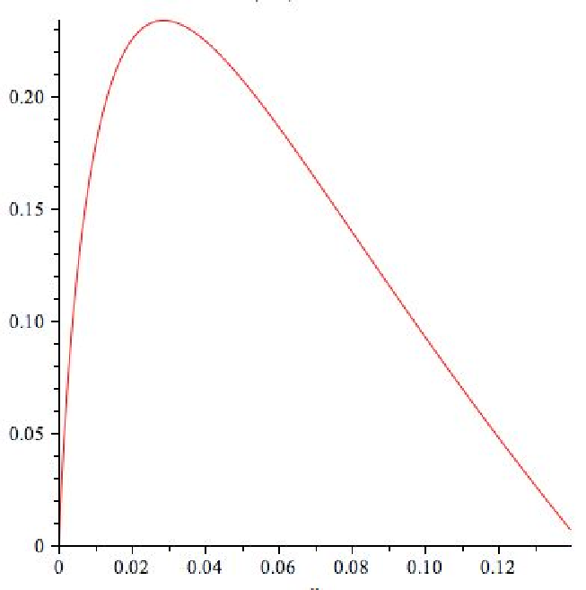
Refer to caption — Figure 2: Plot of $\beta^{\beta}-\frac{1}{\beta^{\beta}(1-\beta)^{1-\beta}}\left(\frac{1}{2}-\frac{1}{2}\left(\frac{\beta}{2}\right)^{\frac{43}{3}\beta}\right)$ when $0<\beta\leq\frac{6}{43}$

As this may suggest, the above result result can be improved slightly — but not by very much: The inequality at line (2.25), above, is not satisfied if $c_{4}$ is decreased to $14$ and $\beta_{0}$ increased to $\frac{1}{7}$ .

In order to see one more example of this process let us consider the case that $q\geq 3$ . An application of the technique described above establishes the following.

Lemma 2.7.

If $q=3$ , $0<\beta\leq\frac{1}{4}$ and $c_{4}\geq 8$ then

\frac{2^{\beta}}{\beta^{\beta}(1-\beta)^{1-\beta}}\left({\textstyle{\frac{1}{3}}}+{\textstyle{\frac{2}{3}}}(3n)^{-c_{4}\beta}\right)\leq\beta^{\beta}.

Proof.

To begin, let us use the process described in Subsection 2.2.1 to establish the above inequality when $0<\beta\leq\frac{1}{5}$ . It follows by part (b) of Lemma 2.2 that $(1-x)^{-(1-x)}\leq x^{\gamma x}$ when $0<x\leq\frac{1}{5}$ and $\gamma=-\frac{23}{40}$ , so that $\gamma$ can be set to have this value when this process is applied. It follows by Lemma 2.3 that if $q=3$ and $\delta=-\frac{9}{20}$ then $(q-1)^{x}\leq x^{\delta x}$ when $0<x\leq\frac{1}{5}$ , so $\delta$ can be set to be $-\frac{9}{20}$ in this argument. In this case

c_{4}-\left(\frac{2q}{q-1}-\frac{\delta}{q-1}-\frac{q\gamma}{q-1}\right)=\frac{313}{80}>0,

so that the condition at line (2.19) is satisfied. Since $0<\frac{1}{5}<\frac{1}{4}\leq\frac{1}{e}$ , it now suffices to note that $f_{1}(\frac{1}{5})>0.0008$ and $f_{1}(\frac{1}{4})<-0.03$ — for it then follows by Lemma 2.4 that the inequality in the claim is satisfied when $0<\beta\leq\frac{1}{5}$ .

The process described in Subsection 2.2.2 can now be used to establish the above inequality when $\frac{1}{5}\leq\beta\leq\frac{1}{4}$ , completing the proof. Since $F_{1}^{\prime}\left(\frac{1}{4}\right)<-2.1$ the function $F_{1}$ is decreasing over this interval, for every choice of $\eta$ . Since $\frac{1}{4}<\frac{6}{7}=1+\frac{1}{1-8}$ and $F_{2}^{\prime}\left(\frac{1}{4}\right)>9$ , the function $F_{2}$ is increasing over this interval for every choice of $\eta$ .

It now suffices to confirm that if $\eta=\frac{39}{40}$ then $F_{1}\left(\frac{6}{25}\right)>0.01$ and $F_{2}\left(\frac{1}{5}\right)>0.08$ , so that $F_{1}$ and $F_{2}$ are both non-negative over the interval $\frac{1}{5}\leq\beta\leq\frac{6}{25}$ .

It then suffices to confirm that if $\eta=\frac{123}{125}$ then $F_{1}\left(\frac{1}{4}\right)>0.0002$ and $F_{2}\left(\frac{6}{25}\right)>0.05$ , so that $F_{1}$ and $F_{2}$ are both non-negative over the interval $\frac{6}{25}\leq x\leq\frac{1}{4}$ , as needed to complete the proof. ∎

It now follows that

\rho_{0}\leq\sum_{1\leq j<k\beta_{0}}\beta^{k\beta}\quad\text{if $q=3$, $\beta_{0}=\frac{1}{4}$, and $c_{4}\geq 4$.}

(2.26)

A plot of the function $\beta^{\beta}-\frac{2^{\beta}}{\beta^{\beta}(1-\beta)^{1-\beta}}\left(\frac{1}{3}+\frac{2}{3}\left(\frac{\beta}{3}\right)^{8\beta}\right)$ , when $0<\beta\leq\frac{1}{4}$ , is shown in Figure 3.

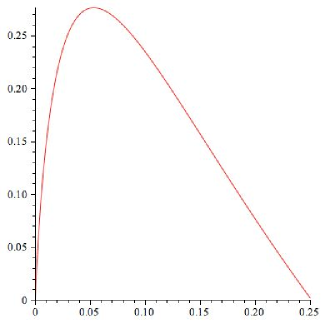
Once again, this suggests that the above result cannot be improved by very much.

Appendix B include details of analyses for additional field sizes as well — as summarized in Figure 4 on page 4. A Maple worksheet, that can be used to check these details, is available online at

http://www.cpsc.ucalgary.ca/~eberly/Research/sparse_conditioner.mw.

$q$	$c_{4}$	$\beta_{0}$	$q$	$c_{4}$	$\beta_{0}$	$q$	$c_{4}$	$\beta_{0}$
$2$	$\frac{43}{3}$	$\frac{6}{43}$	$9$	$\frac{11}{3}$	$\frac{6}{11}$	$47$ – $59$	$\frac{7}{3}$	$\frac{6}{7}$
$3$	$8$	$\frac{1}{4}$	$11$	$\frac{7}{2}$	$\frac{4}{7}$	$61$ – $71$	$\frac{9}{4}$	$\frac{8}{9}$
$4$	$\frac{25}{4}$	$\frac{8}{25}$	$13$	$\frac{10}{3}$	$\frac{3}{5}$	$73$ – $83$	$\frac{11}{5}$	$\frac{10}{11}$
$5$	$\frac{16}{3}$	$\frac{3}{8}$	$16$ – $19$	$3$	$\frac{2}{3}$	$\geq 89$	$\frac{13}{6}$	$\frac{12}{13}$
$7$	$\frac{13}{3}$	$\frac{6}{13}$	$23$ – $29$	$\frac{8}{3}$	$\frac{3}{4}$
$8$	$4$	$\frac{1}{2}$	$31$ – $43$	$\frac{5}{2}$	$\frac{4}{5}$

Figure 4: Choices of

c_{4}

and

\beta_{0}

for Various Field Sizes

It follows from this that

\rho_{0}\leq\sum_{1\leq j<k\beta_{0}}\beta^{k\beta}

for each of the choices of $q$ , $\beta_{0}$ and $c_{4}$ given in Figure 4.

2.3 Asymptotic Results: Choice of Field Size

The objective of this next subsection is to identify bounds on the sizes of primes allowing the inequality at line (2.12) to be established when $c_{4}$ is closer to $2$ . Suppose, in particular, that $N$ is an integer such that $N\geq 18$ and that

c_{4}=2+{\textstyle{\frac{1}{N}}}\qquad\text{and}\qquad q\geq 16N+9.

(2.27)

Consider now the function

\begin{split}g(\beta)&=\frac{\left(\frac{(q-1)^{\beta}}{\beta^{\beta}(1-\beta)^{1-\beta}}\right)\left(\frac{1}{q}+\left(\frac{q-1}{q}\right)\left(\frac{\beta}{q}\right)^{c\beta}\right)}{\beta^{\beta}}\\ &=\frac{(q-1)^{\beta}}{\beta^{2\beta}(1-\beta)^{1-\beta}}\left(\frac{1}{q}+\left(\frac{q-1}{q}\right)\left(\frac{\beta}{q}\right)^{c_{4}\beta}\right)\end{split}

(2.28)

noting — by the inequality at line (2.13) — that the inequality at line (2.12) is satisfied if $g(\beta)\leq 1$ when $0<\beta\leq\beta_{0}=\frac{2}{c_{4}}$ .

Consider, as well the function

\begin{split}h(\beta)&=\ln g(\beta)\\ &=\beta\ln(q-1)-2\beta\ln\beta-(1-\beta)\ln(1-\beta)\\ &\hskip 72.26999pt+\ln\left(\frac{1}{q}+\left(\frac{q-1}{q}\right)\left(\frac{\beta}{q}\right)^{c_{4}\beta}\right)\end{split}

(2.29)

observing that

h^{\prime}(\beta)=\ln(q-1)-2\ln\beta+\ln(1-\beta)-1+\frac{H(\beta)}{H(\beta)+1}(c_{4}+c_{4}\ln\beta-c_{4}\ln q)

(2.30)

where

H(\beta)=(q-1)\left(\frac{\beta}{q}\right)^{c_{4}\beta}.

(2.31)

Lemma 2.8.

If $0<\beta\leq\frac{1}{50c_{4}\ln q}$ then $g(\beta)\leq 1$ .

Proof.

It is easily checked that $\displaystyle{\lim_{\beta\rightarrow 0^{+}}g(\beta)}=1$ and $\displaystyle{\lim_{\beta\rightarrow 0^{+}}h(\beta)}=0$ . The claim can therefore be established by showing that $h^{\prime}(\beta)<0$ when $0<\beta\leq\frac{1}{50c_{4}\ln q}$ .

Consider the above function $H(\beta)$ , recalling as well that

\frac{x}{1+x}\leq\ln(1+x)\leq x,

(2.32)

for any real number $x$ such that $x>-1$ . Replacing $x$ with $-x$ (where $x<1$ ), one has that

-\frac{x}{1-x}\leq\ln(1-x)\leq-x

as well, and replacing $x$ with $1-x$ (where, once again $x<1$ ) one has that

1-\frac{1}{x}\leq\ln x\leq x-1.

It follows from this that (for $0<x<1$ )

x-1\leq x\ln x\leq x^{2}-x,

so that

e^{x-1}\leq x^{x}\leq e^{x^{2}-x}\leq 1

when $0<x\leq 1$ . It follows from the definition of $H(\beta)$ at line (2.31) that

$\displaystyle H(\beta)$	$\displaystyle\geq(q-1)\frac{e^{(\beta-1)c_{4}}}{q^{c_{4}\beta}}$
	$\displaystyle\geq(q-1)\frac{e^{-c_{4}}}{q^{c_{4}\beta}}$
	$\displaystyle=(1-q^{-1})e^{-c_{4}}q^{1-c_{4}\beta}$
	$\displaystyle\geq(1-q^{-1})e^{-\frac{37}{18}}q^{1-c_{4}\beta}$	(since $N\geq 18$ , so that $c_{4}\leq\frac{37}{18}$ )
	$\displaystyle\geq\frac{296}{297}\frac{e^{-\frac{37}{18}}}{q^{c_{4}\beta}}q$	(since $q=16N+9\geq 297$ )
	$\displaystyle\geq\frac{296}{297}\frac{e^{-\frac{37}{18}}}{q^{\frac{1}{50\ln q}}}q$	(since $\beta\leq\frac{1}{50c_{4}\ln q}$ )
	$\displaystyle=\frac{296}{297}e^{-\frac{37}{18}-\frac{1}{50}}q$
	$\displaystyle>\frac{q}{8}$
	$\displaystyle\geq 2N+1$	(since $q\geq 16N+9$ ).

It follows that

\frac{H(\beta)}{H(\beta)+1}=1-(H(\beta)+1)^{-1}\geq 1-(2N+1)^{-1}=\frac{2N}{2N+1}.

Note, as well that $c_{4}+c_{4}\ln\beta-c_{4}\ln q=c_{4}\left(1+\ln\textstyle{\frac{\beta}{q}}\right)<c_{4}\left(1+\ln\textstyle{\frac{1}{q}}\right)<0$ . It now follows by the equation at line (2.30) that

$\displaystyle h^{\prime}(\beta)$	$\displaystyle=\ln(q-1)-2\ln\beta+\ln(1-\beta)-1+\frac{H(\beta)}{H(\beta)+1}(c_{4}+c_{4}\ln\beta-c_{4}\ln q)$
	$\displaystyle\leq\ln(q-1)-2\ln\beta+\ln(1-\beta)-1+\textstyle{\frac{2N}{2N+1}}(c_{4}+c_{4}\ln\beta-c_{4}\ln q)$
	$\displaystyle=\ln(q-1)-2\ln\beta+\ln(1-\beta)-1+2(1+\ln\beta-\ln q)$	(since $c_{4}=2+\frac{1}{N}=\frac{2N+1}{N}$ )
	$\displaystyle<-\ln q+\ln(1-\beta)+1<0,$

as required. ∎

A different approach is required for larger values of $\beta$ because $h^{\prime}(\beta)$ is eventually positive. Note that $g(\beta)=g_{1}(\beta)+g_{2}(\beta)$ , where

g_{1}(\beta)=\frac{(q-1)^{\beta}}{\beta^{2\beta}(1-\beta)^{1-\beta}}\cdot\frac{1}{q}=q^{-1}(q-1)^{\beta}\cdot\frac{(1-\beta)^{\beta-1}}{\beta^{2\beta}}

(2.33)

and

g_{2}(\beta)=\frac{(q-1)^{\beta}}{\beta^{2\beta}(1-\beta)^{1-\beta}}\cdot\left(\frac{q-1}{q}\right)\left(\frac{\beta}{q}\right)^{c_{4}\beta}=\left(1-\frac{1}{q}\right)\frac{\beta^{\beta/N}}{\left(\frac{q^{c_{4}-1}}{1-\beta}\right)^{\beta}(1-\beta)}.

(2.34)

Lemma 2.9.

If $\frac{1}{50c_{4}\ln q}\leq\beta\leq\frac{7}{8}$ then $g(\beta)\leq 1$ .

Proof.

Consider first the function

k(x)=\frac{(1-x)^{x-1}}{x^{2x}}

and

\ell(x)=\ln k(x)=(x-1)\ln(1-x)-2x\ln x,

noting that

\ell^{\prime}(x)=\ln(1-x)-2\ln x-1

and

\ell^{\prime\prime}(x)=-\frac{1}{1-x}-\frac{2}{x},

so that $\ell^{\prime\prime}(x)<0$ when $0<x<1$ . Note that $\ell^{\prime}(x)=0$ when

\frac{1-x}{x^{2}}=e,

that is, when $ex^{2}+x-1=0$ . Applying the quadratic equation, one can see that the functions $k(x)$ and $\ell(x)$ are both increasing when $0<x<\frac{-1+\sqrt{1+4e}}{2e}$ , and decreasing when $\frac{1+\sqrt{1+4e}}{2e}<x<1$ . In particular, $k(x)\leq k\left(\frac{-1+\sqrt{1+4e}}{2e}\right)<3$ for $0<x<1$ .

This be used to obtain upper bounds for the function $g_{1}$ , shown at line (2.33), above, over various intervals. Suppose, in particular, that $k(\beta)\leq\delta$ when $\Delta_{L}<\beta\leq\Delta_{H}$ for constants $\delta$ , $\Delta_{L}$ and $\Delta_{H}$ such that $0<\Delta_{L}<\Delta_{H}<1$ . It follows that if $\Delta_{L}<\beta\leq\Delta_{H}$ then

g_{1}(\beta)\leq\delta q^{-1}(q-1)^{\beta}\leq{\textstyle{\frac{\delta}{297}}}296^{\beta}\quad\text{when $\beta\leq\textstyle{\frac{7}{8}}$}

since $q\geq 297$ ; this upper bound for $g_{2}(\beta)$ is increasing with $\beta$ .

Note, as well, that, since $\frac{x}{1+x}\leq\ln(1+x)\leq x$ for any real number $x$ such that $x>-1$ , $-\frac{x}{1-x}\leq\ln(1-x)\leq-x$ for any real number $x$ such that $0<x<1$ . Consequently $-x\leq(1-x)\ln(1-x)\leq-x+x^{2}$ , so that

e^{-x}\leq(1-x)^{1-x}\leq e^{-x+x^{2}},

and (replacing $x$ with $1-x$ , and applying the bounds for $(1-x)^{1-x}$ )

e^{1-x}\leq x^{x}\leq e^{-x+x^{2}}

when $0<x<1$ . Thus, if $g_{2}(\beta)$ is as given at line (2.34), above, then

$\displaystyle g_{2}(\beta)$	$\displaystyle=\left(1-\frac{1}{q}\right)\frac{\beta^{\beta/N}}{\left(\frac{q^{c_{4}-1}}{1-\beta}\right)^{\beta}(1-\beta)}$
	$\displaystyle\leq\left(1-\frac{1}{q}\right)\frac{1}{q^{(c_{4}-1)\beta}(1-\beta)^{1-\beta}}$	(since $\beta^{\beta}\leq e^{-\beta+\beta^{2}}\leq 1$ )
	$\displaystyle\leq\left(1-\frac{1}{q}\right)\left(\frac{e}{q^{c_{4}-1}}\right)^{\beta}$	(since $(1-\beta)^{1-\beta}\geq e^{-\beta}$ )
	$\displaystyle<\left(1-\frac{1}{q}\right)\left(\frac{e}{q}\right)^{\beta}$	(since $c_{4}>2$ )
	$\displaystyle\leq{\textstyle{\frac{296}{297}}}\left({\textstyle{\frac{e}{297}}}\right)^{\beta}$	(since $q\geq 297$ ).

Since $q>e$ , this upper bound for $g_{2}(\beta)$ is certainly decreasing as $\beta$ increases.

It follows by Lemma 2.8 that $g(\beta)=g_{1}(\beta)+g_{2}(\beta)<1$ when $\beta=\frac{1}{50c_{4}\ln q}$ . Now

	$\displaystyle g_{2}\left({\textstyle{\frac{1}{50c_{4}\ln q}}}\right)$	$\displaystyle\leq\left({\textstyle{1-\frac{1}{q}}}\right)\left({\textstyle{\frac{e}{q}}}\right)^{\frac{1}{50c_{4}\ln q}}$
		$\displaystyle\leq\left({\textstyle{1-\frac{1}{q}}}\right)\left(e^{\frac{1}{50c_{4}}}\right)^{\frac{1}{\ln q}-1}$
		$\displaystyle\leq\left(e^{\frac{1}{50c_{4}}}\right)^{\frac{1}{\ln q}-1}.$

Since $e^{\frac{1}{50c_{4}}}>1$ , $q\geq 297$ , and the above exponent $\frac{1}{\ln q}-1$ decreases as $q$ increases, it now follows that

g_{2}\left({\textstyle{\frac{1}{50c_{4}\ln q}}}\right)\leq\left(e^{\frac{1}{50c_{4}}}\right)^{\frac{1}{\ln 297}-1}.

Now, since $N\geq 18$ , $c_{4}\leq\frac{37}{18}$ and $\frac{1}{50c_{4}}\geq\frac{9}{925}$ . Since the exponent in the above expression is negative, it now follows that

g_{2}\left({\textstyle{\frac{1}{50c_{4}\ln q}}}\right)\leq\left(e^{\frac{9}{925}}\right)^{\frac{1}{\ln 297}-1}<\frac{397}{400}.

Since $g_{2}$ is decreasing with $\beta$ and $g_{1}$ is increasing with $\beta$ , it now suffices to choose a value $\gamma$ such that $\frac{1}{50c_{4}\ln q}<\gamma\leq\frac{7}{8}$ , and $g_{1}(\gamma)\leq\frac{3}{400}$ in order to conclude that $g(\beta)=g_{1}(\beta)+g_{2}(\beta)\leq 1$ when $\frac{1}{50c_{4}\ln q}\leq\beta\leq\gamma$ .

Suppose now that $\gamma\leq\frac{1}{8}$ as well; then $k(\gamma)\leq k\left(\frac{1}{8}\right)\leq 2$ so that $g_{1}(\beta)\leq\frac{2}{297}296^{\beta}$ . It follows from that that if $\gamma=\frac{1}{75}$ then $\frac{1}{50c_{4}\ln q}<\frac{1}{75}<\frac{1}{8}$ and $g_{1}(\gamma)<\frac{3}{400}$ , as required to conclude that $g(\beta)<1$ when $\frac{1}{50c_{4}\ln q}\leq\beta\leq\frac{1}{75}$ .

Note next that $g_{2}\left(\frac{1}{75}\right)\leq\frac{296}{297}\left(\frac{e}{297}\right)^{\frac{1}{75}}<\frac{19}{20}$ . Since $g_{2}$ is decreasing with $\beta$ and $g_{1}$ is increasing with $\beta$ , it suffices to choose a value $\widehat{\gamma}$ such that $\frac{1}{75}<\widehat{\gamma}\leq\frac{7}{8}$ and $g(\widehat{\gamma})<\frac{1}{20}$ in order to conclude that $g(\beta)\leq 1$ when $\frac{1}{75}\leq\beta\leq\widehat{\gamma}$ as well.

As noted above, $k(\beta)<3$ when $0<\beta<1$ , and it follows that $g_{1}(\beta)\leq\frac{3}{297}296^{\beta}$ for all such $\beta$ . It follows from this that if $\widehat{\gamma}=\frac{1}{4}$ then $g_{1}(\gamma)<\frac{1}{20}$ , as needed to conclude that $g(\beta)\leq 1$ when $\frac{1}{75}\leq\beta\leq\frac{1}{4}$ .

Now note that $g_{2}(\left(\frac{1}{4}\right)\leq\frac{296}{97}\left(\frac{e}{297}\right)^{\frac{1}{4}}<\frac{1}{3}$ . Since $g_{2}$ is decreasing with $\beta$ and $g_{1}$ is increasing with $\beta$ it suffices to choose a value $\widetilde{\gamma}$ such that $\frac{1}{4}<\widetilde{\gamma}\leq\frac{7}{8}$ and $g(1)(\widetilde{\gamma})\leq\frac{2}{3}$ in order to conclude that $g(\beta)\leq 1$ when $\frac{1}{4}\leq\beta\leq\widetilde{\gamma}$ .

Once again, $g_{1}(\widetilde{\gamma})\leq\frac{3}{297}296^{\widetilde{\gamma}}$ , and this suffices to set $\widetilde{\gamma}=\frac{2}{3}$ in order to ensure that $g_{1}(\widetilde{\gamma})<\frac{2}{3}$ , as needed.

Now $g_{2}(\left(\widetilde{\beta}\right)=g_{2}\left(\frac{2}{3}\right)<\frac{1}{20}$ , so it suffices to choose $\overline{\gamma}$ such that $\frac{2}{3}<\overline{\gamma}\leq\frac{7}{8}$ and $g_{1}(\overline{\gamma})\leq\frac{19}{20}$ in order to ensure that $g(\beta)\leq 1$ when $\frac{2}{3}\leq\beta\overline{\gamma}$ . Now, $k(x)\leq\frac{5}{2}$ when $\frac{2}{3}\leq x\leq\frac{7}{8}$ , so that $g_{1}(x)\leq\frac{5}{2}\cdot\frac{1}{297}\cdot 296^{x}$ for all $x$ in this range, and this can be used to establish that one can set $\overline{\beta}=\frac{4}{5}$ in order to ensure that the desired conditions are met.

Finally, $g_{2}\left(\frac{4}{5}\right)<\frac{23}{1000}$ and $k(x)<\frac{99}{50}$ when $\frac{4}{5}\leq x\leq\frac{7}{8}$ . This can be used to establish that $g_{1}(\left(\frac{7}{8}\right)<\frac{977}{1000}$ , as needed to establish that $g(\beta)\leq 1$ when $\frac{4}{5}\leq\beta\leq\frac{7}{8}$ and complete the proof of the claim. ∎

Once again the functions $h(\beta)$ , $h^{\prime}(\beta)$ and $H(\beta)$ , shown at lines (2.29)–(2.31), are of use to prove the desired result for larger values of $\beta$ .

Lemma 2.10.

If $\frac{7}{8}\leq\beta\leq\frac{2N}{2N+1}$ then $g(\beta)\leq 1$ .

Proof.

Consider the functions $h(\beta)$ , $h^{\prime}(\beta)$ and $H(\beta)$ . Note first that if $\frac{7}{8}\leq\beta\leq\frac{2N}{2N+1}$ then

$\displaystyle H(\beta)$	$\displaystyle=(q-1)\left({\textstyle{\frac{\beta}{q}}}\right)^{c_{4}\beta}$
	$\displaystyle\leq(q-1)\left({\textstyle{\frac{1}{q}}}\right)^{c_{4}\beta}$	(since $\beta<1$ , $q>0$ ,and $c_{4}\beta>1$ )
	$\displaystyle\leq q^{1-c_{4}\beta}$
	$\displaystyle\leq q^{-\frac{3}{4}}$	(since $c_{4}\geq 2$ and $\beta\geq\frac{7}{8}$ , so that $1-c_{4}\beta\leq-\frac{3}{4}$ ).

Since $H(\beta)\geq 0$ as well, it follows that

\frac{H(\beta)}{H(\beta)+1}\leq H(\beta)\leq q^{-\frac{3}{4}}

as well. Since $c_{4}=2+\frac{1}{N}\leq 2+\frac{1}{18}=\frac{37}{18}$ ,

c_{4}\frac{H(\beta)}{H(\beta)+1}\leq\frac{37}{18}\cdot q^{-\frac{3}{4}}.

Since $1+\ln\beta-\ln q<0$ it now follows that

$\displaystyle h^{\prime}(\beta)$	$\displaystyle=\ln(q-1)-2\ln\beta+\ln(1-\beta)-1+\frac{H(\beta)}{H(\beta)+1}(c_{4}+c_{4}\ln\beta-c_{4}\ln q)$
	$\displaystyle\geq\ln(q-1)-2\ln\beta+\ln(1-\beta)-1+\frac{37}{18}\cdot q^{-\frac{3}{4}}(1+\ln\beta+\ln q)$
	$\displaystyle\geq\ln(16N+8)-2\ln\beta+\ln\left(\frac{1}{2N+1}\right)-1+\frac{37}{18}\cdot q^{-\frac{3}{4}}(1+\ln\beta+\ln q)$	(since $q-1\geq 16N+8$ and $1-\beta\geq\frac{1}{2N+1}$ )
	$\displaystyle=\ln 8-2\ln\beta-1+\frac{37}{18}\cdot q^{-\frac{3}{4}}(1+\ln\beta+\ln q)$
	$\displaystyle=(\ln 8-1+{\textstyle{\frac{37}{18}}}\cdot q^{-\frac{3}{4}}(1+\ln q))-(2-{\textstyle{\frac{37}{18}}}\cdot q^{-\frac{3}{4}})\ln\beta$
	$\displaystyle\geq{\textstyle{\frac{9}{10}}}-(2-{\textstyle{\frac{37}{18}}}\cdot q^{-\frac{3}{4}})\ln\beta$	(since $\ln 8-1+{\textstyle{\frac{37}{18}}}\cdot q^{-\frac{3}{4}}(1+\ln q)\geq\ln 8-1+{\textstyle{\frac{37}{18}}}\cdot 267^{-\frac{3}{4}}(1+\ln 267)\leq{\textstyle{\frac{9}{10}}}$ )
	$\displaystyle\geq{\textstyle{\frac{9}{10}}}$	(since $\ln\beta<0$ and $2-{\textstyle{\frac{37}{18}}}\cdot q^{-\frac{3}{4}}\geq 2-{\textstyle{\frac{37}{18}}}\cdot 267^{-\frac{3}{4}}\geq{\textstyle{\frac{19}{10}}}>0$ )
	$\displaystyle>0.$

Thus the function $h(\beta)$ is increasing over the interval $\frac{7}{8}\leq\beta\leq\frac{2N}{2N+1}$ . Since $h(\beta)=\ln g(\beta)$ , the function $g(\beta)$ is increasing as well — and it suffices to confirm that $g\left(\frac{2N}{2N+1}\right)\leq 1$ in order to establish the claim.

Now recall that $g\left(\frac{2N}{2N+1}\right)=g_{1}\left(\frac{2N}{2N+1}\right)+g_{2}\left(\frac{2N}{2N+1}\right)$ , for the functions $g_{1}(\beta)$ and $g_{2}(\beta)$ as defined at lines (2.33) and (2.34) respectively. Applying these definitions one can see that

$\displaystyle g_{1}\left({\textstyle{\frac{2N}{2N+1}}}\right)$	$\displaystyle=q^{-1}(q-1)^{\frac{2N}{2N+1}}\frac{\left({\textstyle{\frac{1}{2N+1}}}\right)^{-\frac{1}{2N+1}}}{\left({\textstyle{\frac{2N}{2N+1}}}\right)^{\frac{4N}{2N+1}}}$
	$\displaystyle=\left(1-{\textstyle{\frac{1}{q}}}\right)\frac{(q-1)^{-\frac{1}{2N+1}}\cdot\left({\textstyle{\frac{1}{2N+1}}}\right)^{-\frac{1}{2N+1}}}{\left({\textstyle{\frac{2N}{2N+1}}}\right)^{\frac{4N}{2N+1}}}$
	$\displaystyle\leq\frac{16N+8}{16N+9}\cdot\frac{\left((16N+8)\cdot\left({\textstyle{\frac{1}{2N+1}}}\right)\right)^{-\frac{1}{2N+1}}}{\left({\textstyle{\frac{2N}{2N+1}}}\right)^{\frac{4N}{2N+1}}}$	(since $q\geq 16N+9$ )
	$\displaystyle=\frac{16N+8}{16N+9}\cdot\frac{8^{-\frac{1}{2N+1}}}{\left({\textstyle{\frac{2N}{2N+1}}}\right)^{\frac{4N}{2N+1}}}$
	$\displaystyle\leq\frac{16N+8}{16N+9}\cdot\frac{8^{-\frac{1}{2N+1}}}{e^{-\frac{2}{2N+1}}}$	(since ${\textstyle{\left(\frac{2N}{2N+1}\right)}}^{\frac{4N}{2N+1}}\geq e^{-\frac{2}{2N+1}}$ )
	$\displaystyle=\frac{16N+8}{16N+9}\cdot\left(\frac{e^{2}}{8}\right)^{\frac{1}{2N+1}}$
	$\displaystyle\leq\frac{16N+8}{16N+9}$	(since $\textstyle{\frac{e^{2}}{8}}<1$ )

and

$\displaystyle g_{2}\left({\textstyle{\frac{2N}{2N+1}}}\right)$	$\displaystyle=\left(1-{\textstyle{\frac{1}{q}}}\right)\frac{\left({\textstyle{\frac{2N}{2N+1}}}\right)^{\frac{2}{2N+1}}}{\left(\frac{q^{\frac{N+1}{N}}}{\frac{1}{2N+1}}\right)^{\frac{2N}{2N+1}}\left({\textstyle{\frac{1}{2N+1}}}\right)}$
	$\displaystyle=\left(1-{\textstyle{\frac{1}{q}}}\right)\frac{\left({\textstyle{\frac{2N}{2N+1}}}\right)^{\frac{2}{2N+1}}}{\left(q^{\frac{N+1}{N}}\right)^{\frac{2N}{2N+1}}\left({\textstyle{\frac{1}{2N+1}}}\right)^{\frac{1}{2N+1}}}$
	$\displaystyle=\left(1-{\textstyle{\frac{1}{q}}}\right)\frac{\left({\textstyle{\frac{(2N)^{2}}{2N+1}}}\right)^{\frac{1}{2N+1}}q^{-\frac{1}{2N+1}}}{q}$
	$\displaystyle\leq\left(1-{\textstyle{\frac{1}{q}}}\right)\frac{\left({\textstyle{\frac{(2N)^{2}}{(2N+1)^{2}}}}\right)^{\frac{1}{2N+1}}}{q}$	(since $q\geq 16N+9\geq 2N+1$ )
	$\displaystyle\leq\left(1-{\textstyle{\frac{1}{q}}}\right)\cdot{\textstyle{\frac{1}{q}}}$
	$\displaystyle\leq\frac{1}{q}$
	$\displaystyle\leq\frac{1}{16N+9}$	(since $q\geq 16N+9$ )

as needed to establish that $g\left(\frac{2N}{2N+1}\right)\leq 1$ and complete the proof. ∎

The following is now a straightforward consequence of Lemmas 2.8–2.10.

Corollary 2.11.

If $N\geq 18$ , $c_{4}$ and $q$ are as shown at line (2.27), and $\beta_{0}=\frac{2}{c_{4}}=\frac{2N}{2N+1}$ , the the inequality at line (2.12) is satisfied.

2.4 Splitting the Sum to Get a Better Bound for $\boldsymbol{\rho_{0}}$

Let $\epsilon$ be a positive constant. Suppose now that $\Delta$ is a positive integer whose depends on $\epsilon$ and the field size $q$ . It follows from the above (for appropriate choices of $q$ , $\beta_{0}$ and $c_{4}$ ) that

$\displaystyle\rho_{0}$	$\displaystyle\leq\sum_{1\leq j<k\beta_{0}}\beta^{k\beta}$
	$\displaystyle=\sum_{1\leq j<k\beta_{0}}\left(\frac{j}{k}\right)^{j}$	(since $\beta=\frac{j}{k}$ )
	$\displaystyle=\zeta+\theta,$

where

\zeta=\sum_{1\leq j\leq\Delta}\left(\frac{j}{k}\right)^{j}

(2.35)

and

\theta=\sum_{\Delta<j<k\beta_{0}}\left(\frac{j}{k}\right)^{j}.

(2.36)

It follows from the above that

	$\displaystyle\theta$	$\displaystyle\leq\sum_{\Delta<j\leq k\beta_{0}}\left(\frac{j}{k}\right)^{j}$
		$\displaystyle\leq\sum_{\Delta<j\leq k\beta_{0}}\beta_{0}^{j}$
		$\displaystyle\leq\beta_{0}^{\Delta+1}\sum_{j\geq 0}\beta_{0}^{j}$
		$\displaystyle=\frac{\beta_{0}^{\Delta+1}}{1-\beta_{0}}$
		$\displaystyle\leq{\textstyle{\frac{1}{10}}}\epsilon$

provided that

\Delta\geq\frac{\ln(\epsilon^{-1})+\ln 10-\ln(1-\beta_{0})}{\ln(1/\beta_{0})}-1.

Choices of $\Delta$ that satisfy this inequality for various field sizes (and corresponding choices of $\beta_{0}$ ) are shown in Figure 5 on page 5.

$q$	$\beta_{0}$	$\Delta$	$q$	$\beta_{0}$	$\Delta$	$q$	$\beta_{0}$	$\Delta$
$2$	$\frac{6}{43}$	$\lceil\frac{51}{100}\ln(\epsilon^{-1})+\frac{1}{4}\rceil$	$9$	$\frac{6}{11}$	$\lceil\frac{33}{20}\ln(\epsilon^{-1})+\frac{41}{10}\rceil$	$47$ – $59$	$\frac{6}{7}$	$\lceil\frac{13}{2}\ln(\epsilon^{-1})+\frac{133}{5}\rceil$
$3$	$\frac{1}{4}$	$\lceil\frac{73}{100}\ln(\epsilon^{-1})+\frac{9}{10}\rceil$	$11$	$\frac{4}{7}$	$\lceil\frac{179}{100}\ln(\epsilon^{-1})+\frac{47}{10}\rceil$	$61$ – $71$	$\frac{8}{9}$	$\lceil\frac{17}{2}\ln(\epsilon^{-1})+\frac{149}{4}\rceil$
$4$	$\frac{8}{25}$	$\lceil\frac{22}{25}\ln(\epsilon^{-1})+\frac{7}{5}\rceil$	$13$	$\frac{3}{5}$	$\lceil\frac{49}{25}\ln(\epsilon^{-1})+\frac{107}{20}\rceil$	$73$ – $83$	$\frac{10}{11}$	$\lceil\frac{21}{2}\ln(\epsilon^{-1})+\frac{242}{5}\rceil$
$5$	$\frac{3}{8}$	$\lceil\frac{51}{50}\ln(\epsilon^{-1})+\frac{19}{10}\rceil$	$16$ – $19$	$\frac{2}{3}$	$\lceil\frac{99}{40}\ln(\epsilon^{-1})+\frac{37}{5}\rceil$	$\geq 89$	$\frac{12}{13}$	$\lceil\frac{25}{2}\ln(\epsilon^{-1})+\frac{599}{10}\rceil$
$7$	$\frac{6}{13}$	$\lceil\frac{13}{10}\ln(\epsilon^{-1})+\frac{14}{5}\rceil$	$23$ – $29$	$\frac{3}{4}$	$\lceil\frac{87}{25}\ln(\epsilon^{-1})+\frac{119}{10}\rceil$
$8$	$\frac{1}{2}$	$\lceil\frac{29}{20}\ln(\epsilon^{-1})+\frac{17}{5}\rceil$	$31$ – $43$	$\frac{4}{5}$	$\lceil\frac{9}{2}\ln(\epsilon^{-1})+\frac{50}{3}\rceil$

Figure 5: Choices of

\Delta

for Various Field Sizes

When $N\geq 18$ and $\beta_{0}=\frac{2N}{2N+1}$ (as in Subsection 2.3)

$\displaystyle\frac{\ln(\epsilon^{-1})+\ln 10-\ln(1-\beta_{0})}{\ln(1/\beta_{0}}-1$	$\displaystyle=\frac{\ln(\epsilon^{-1}+\ln 10-\ln\left({\textstyle{\frac{1}{2N+1}}}\right)}{\ln\left(1+{\textstyle{\frac{1}{2N}}}\right)}-1$
	$\displaystyle\leq\frac{\ln(\epsilon^{-1})+\ln 10+\ln(2N+1)}{{\textstyle{\frac{1}{2N+1}}}}-1$	(since $\ln\left(1+\frac{1}{2N}\right)\geq\frac{1}{2N+1}$ )
	$\displaystyle=(2N+1)\ln(\epsilon^{-1})+(2N+1)\ln(2N+1)+(2N+1)\ln 10-1.$

It therefore suffices to ensure that

\Delta\geq\lceil(2N+1)\ln(\epsilon^{-1})+(2N+1)\ln(2N+1)+(2N+1)\ln 10-1\rceil

in this case.

It also follows from the above that

	$\displaystyle\zeta$	$\displaystyle\leq\sum_{1\leq j\leq\Delta}\left(\frac{j}{k}\right)^{j}$
		$\displaystyle\leq\sum_{1\leq j\leq\Delta}\left(\frac{\Delta}{k}\right)^{j}$
		$\displaystyle<\sum_{j\geq 1}\left(\frac{\Delta}{k}\right)^{j}$
		$\displaystyle=\frac{\Delta/k}{1-\Delta/k}$
		$\displaystyle\leq\textstyle{\frac{4}{5}}\epsilon$

provided that $k\geq\lceil(\frac{5}{4}\epsilon^{-1}+1)\Delta\rceil$ , and this is the case if $k\geq\lceil(\frac{5}{4}\epsilon^{-1}+1)(\widehat{\Delta}+1)\rceil$ , where $\Delta=\lceil\widehat{\Delta}\rceil$ . Suitable choices of $k$ for small field sizes are as shown in Figure 6 on page 6.

$q$	Lower Bound for $k$	Bound when $\epsilon=\frac{1}{10}$
$2$	$\lceil\frac{51}{80}\epsilon^{-1}\ln(\epsilon^{-1})+\frac{25}{16}\epsilon^{-1}+\frac{51}{100}\ln(\epsilon^{-1})+\frac{5}{4}\rceil$	$33$
$3$	$\lceil\frac{73}{80}\epsilon^{-1}\ln(\epsilon^{-1})+\frac{19}{8}\epsilon^{-1}+\frac{73}{100}\ln(\epsilon^{-1})+\frac{19}{10}\rceil$	$49$
$4$	$\lceil\frac{11}{10}\epsilon^{-1}\ln(\epsilon^{-1})+3\epsilon^{-1}+\frac{22}{25}\ln(\epsilon^{-1})+\frac{12}{5}\rceil$	$60$
$5$	$\lceil\frac{51}{40}\epsilon^{-1}\ln(\epsilon^{-1})+\frac{29}{8}\epsilon^{-1}+\frac{51}{50}\ln(\epsilon^{-1})+\frac{29}{10}\rceil$	$71$
$7$	$\lceil\frac{13}{8}\epsilon^{-1}\ln(\epsilon^{-1})+\frac{19}{4}\epsilon^{-1}+\frac{13}{10}\ln(\epsilon^{-1})+\frac{19}{5}\rceil$	$92$
$8$	$\lceil\frac{29}{16}\epsilon^{-1}\ln(\epsilon^{-1})+\frac{11}{2}\epsilon^{-1}+\frac{29}{20}\ln(\epsilon^{-1})+\frac{22}{5}\rceil$	$105$
$9$	$\lceil\frac{33}{16}\epsilon^{-1}\ln(\epsilon^{-1})+\frac{51}{8}\epsilon^{-1}+\frac{33}{20}\ln(\epsilon^{-1})+\frac{51}{10}\rceil$	$121$
$11$	$\lceil\frac{179}{80}\epsilon^{-1}\ln(\epsilon^{-1})+\frac{57}{8}\epsilon^{-1}+\frac{179}{100}\ln(\epsilon^{-1})+\frac{57}{10}\rceil$	$133$
$13$	$\lceil\frac{49}{20}\epsilon^{-1}\ln(\epsilon^{-1})+\frac{127}{16}\epsilon^{-1}+\frac{49}{25}\ln(\epsilon^{-1})+\frac{127}{20}\rceil$	$147$
$16$ – $19$	$\lceil\frac{99}{32}\epsilon^{-1}\ln(\epsilon^{-1})+\frac{21}{2}\epsilon^{-1}+\frac{99}{40}\ln(\epsilon^{-1})+\frac{42}{5}\rceil$	$191$
$23$ – $29$	$\lceil\frac{87}{20}\epsilon^{-1}\ln(\epsilon^{-1})+\frac{129}{8}\epsilon^{-1}+\frac{87}{25}\ln(\epsilon^{-1})+\frac{129}{10}\rceil$	$283$
$31$ – $43$	$\lceil\frac{45}{8}\epsilon^{-1}\ln(\epsilon^{-1})+\frac{265}{12}\epsilon^{-1}+\frac{9}{2}\ln(\epsilon^{-1})+\frac{53}{3}\rceil$	$379$
$47$ – $59$	$\lceil\frac{65}{8}\epsilon^{-1}\ln(\epsilon^{-1})+\frac{69}{2}\epsilon^{-1}+\frac{13}{2}\ln(\epsilon^{-1})+\frac{138}{5}\rceil$	$575$
$61$ – $71$	$\lceil\frac{85}{8}\epsilon^{-1}\ln(\epsilon^{-1})+\frac{765}{16}\epsilon^{-1}+\frac{17}{2}\ln(\epsilon^{-1})+\frac{153}{4}\rceil$	$781$
$73$ – $83$	$\lceil\frac{105}{8}\epsilon^{-1}\ln(\epsilon^{-1})+\frac{247}{4}\epsilon^{-1}+\frac{21}{2}\ln(\epsilon^{-1})+\frac{247}{5}\rceil$	$994$
$\geq 89$	$\lceil\frac{125}{8}\epsilon^{-1}\ln(\epsilon^{-1})+\frac{609}{8}\epsilon^{-1}+\frac{25}{2}\ln(\epsilon^{-1})+\frac{609}{10}\rceil$	$1211$

Figure 6: Choices of

k

for Various Field Sizes

When $N\geq 18$ , $c_{4}=2+\frac{1}{N}$ , and $\beta_{0}=\frac{2}{c_{4}}=\frac{2N}{2N+1}$ , it suffices that

k\geq\left\lceil\left({\textstyle{\frac{5}{4}}}\epsilon^{-1}+1\right)((2N+1)\ln(\epsilon^{-1})+(2N+1)\ln(2N+1)+(2N+1)\ln 10\right\rceil\\ \in\Theta(\epsilon^{-1}N(\ln(\epsilon^{-1})+\ln N)).

(2.37)

In particular, when $\epsilon=\frac{1}{10}$ , it suffices to ensure that

k\geq\left\lceil(2N+1)\ln(2N+1)={\textstyle{\frac{167}{5}}}\ln(2N+1)\right\rceil.

(2.38)

It now follows that $\rho_{0}\leq\frac{1}{10}\epsilon+\frac{4}{5}\epsilon=\frac{9}{10}\epsilon$ provided that this constraint on $k$ can be satisfied.

2.5 Completion of the Analysis for the Case $\boldsymbol{q\leq n^{2}}$

Suppose next that one wishes to ensure that $\rho_{1}\leq\frac{1}{20}\epsilon$ , so that $\rho\leq\frac{19}{20}\epsilon$ . If the constraint on $k$ , described above, can be satisfied, then it follows by the inequality at line (2.9) that it suffices to choose $c_{2}$ such that $2q^{-c_{2}}\leq\frac{\epsilon}{20}$ , that is,

c_{2}\geq\log_{q}(40\epsilon^{-1})=\frac{\ln(\epsilon^{-1})+\ln 40}{\ln q}.

It remains to choose $c_{2}+\ell$ rows of the $(n+\ell)\times n$ matrix $B$ uniformly and independently from $\textup{{F}}^{1\times n}$ . Suppose that that the set of rows of the original matrix $A$ , and the $k$ “sparse” rows selected as described above, are linearly independent. Then it follows by Lemma 2.1 that (once the remaining rows of $B$ are chosen uniformly and independently) the rank of $B$ is less than $n$ with probability at most $q^{-\ell}$ . Furthermore, if $q\geq 3$ then the top $n$ rows of $B$ are linearly independent — so that we can set $\ell=0$ — with probability at least $1-\frac{1}{q-1}$ . Thus, if we wish to ensure that this probability is at most $\frac{1}{20}\epsilon$ then it suffices to ensure that either

\ell\geq\log_{q}(20\epsilon^{-1})=\textstyle{\frac{\ln(\epsilon^{-1})+\ln 20}{\ln q}}\quad\text{or}\quad q\geq 20\epsilon^{-1}+1\text{ (and $\ell=0$).}

It now follows that if $c_{4}$ , $c_{2}$ and $\ell$ have all been chosen as described above then the probability that $B$ has rank less than $n$ is at most

\rho+\frac{\epsilon}{20}(1-\rho)\leq\rho+\frac{\epsilon}{20}\leq\frac{19\epsilon}{20}+\frac{\epsilon}{20}=\epsilon.

Choices of $c_{2}$ and $\ell$ satisfying the above constraints, along with the constraints at line (2.8), are shown in Figure 7, for the case that $\epsilon=\frac{1}{10}$ .

$q$	$c_{2}$	$\ell$	$q$	$c_{2}$	$\ell$	$q$	$c_{2}$	$\ell$
$2$	$9$	$8$	$5$	$4$	$4$	$16$ – $19$	$3$	$2$
$3$	$6$	$5$	$7$	$4$	$3$	$23$ – $89$	$2$	$2$
$4$	$5$	$4$	$8$ – $13$	$3$	$3$

Figure 7: Choices of

c_{2}

and

\ell

for Various Field Sizes when

\epsilon=\frac{1}{10}

It now suffices to set $\sigma=c_{3}\left(\frac{q-1}{q}\right)=3c_{4}\left(\frac{q-1}{q}\right)$ , for $c_{4}$ as given in Figure 4 and $\tau=c_{2}+\ell$ , for $c_{2}$ and $\ell$ as given in Figure 7, in order to establish the claim in Theorem 1.1 when $k=n-m-c_{2}$ is greater than or equal to the lower bound given in Subsection 2.4 and $q\leq n^{2}$ , for $c_{2}$ as given above. Setting $\upsilon$ to be the sum of $\ell$ and the lower bound for $k$ , described in Subsection 2.4, suffices to establish these claims when $n-m-c_{2}$ is less than the lower bound for $k$ and $q\leq n^{2}$ as well, for $c_{2}$ as above. The values shown in Figure 1 have been obtained using these equations.

Similarly, Theorem 1.2 can be obtained by setting $c_{4}=2+\frac{1}{N}$ for $N\geq 18$ , $c_{3}=3c_{4}=6+\frac{3}{N}$ , $\sigma=c_{3}(1-\frac{1}{q})$ , $c_{2}=\left\lceil\frac{\ln(40\epsilon^{-1})}{\ln q}\right\rceil$ , $\ell=\left\lceil\frac{\ln 20\epsilon^{-1}}{lnq}\right\rceil$ if $\ell\leq 20\epsilon^{-1}+1$ , setting $\ell=0$ otherwise, setting $\tau=c_{2}+\ell$ , and setting $\upsilon$ to the sum of $\ell$ and the lower bound for $k$ described in Subsection 2.4, above.

2.6 Analysis for the Case $\boldsymbol{q>n^{2}}$

A slight variant of the argument from Wiedemann [2] can be applied when $q>n^{2}$ . Since dense linear algebra is certainly adequate for computations on small matrices it will be assumed that $n\geq 7$ , so that $q\geq 49$ .

Suppose, once again, that $A$ is an $m\times n$ matrix over a field F that is either infinite or has size $q>n^{2}$ . Let $\widehat{q}$ be the largest power of a prime that is less than or equal to $n^{2}$ . It suffices to apply the above construction, using the choices of $c_{4}$ , $c_{3}$ , $\beta_{0}$ , $c_{2}$ and $\ell$ appropriate for a field with size $\widehat{q}$ (so that $\ell=0$ ) — except that, after choosing entries of rows that might be nonzero, the remaining entries of the matrix $B$ , to be filled in, should be chosen uniformly and independently from a finite subset $S$ of F with size at least $n^{2}$ , rather than from the finite field with size $\widehat{q}$ .

In order to see that this process is reliable, consider yet another matrix — namely, a matrix $\widehat{B}$ obtained by placing a distinct indeterminate into each row entry that is assigned a value from $S$ , above, instead of $0$ . Let us denote the indeterminate placed into the $i^{\text{th}}$ new row, in column $j$ , by $z_{i,j}$ . Since $\ell=0$ this results in an $n\times n$ matrix whose entries are elements of F and indeterminates. Let $\widehat{f}$ be the determinant of this matrix — a multivariate polynomial with total degree at most $n-m$ , since only $n-m$ rows include indeterminates, and each entry of such a row has total degree at most one.

Since the rows of the $m\times n$ matrix $A$ are linearly independent, there exists a sequence of integers $i_{1},i_{2},\dots,i_{m}$ such that

1\leq i_{1}<i_{2}<\dots<i_{m}\leq n

and such that the $m\times m$ submatrix, including columns $i_{1},i_{2},\dots,i_{m}$ , is nonsingular. Permuting rows of $A$ as needed, we may assume without loss of generality that the entry of the $j^{\text{th}}$ row of $A$ in column $i_{j}$ is nonzero, for $1\leq j\leq m$ . Consequently, if the $j^{\text{th}}$ row of $A$ was replaced by a row whose $i_{j}^{\text{th}}$ entry is $1$ and whose other entries are $0$ , this would result in an $n\times m$ matrix $\widehat{A}$ whose rows are linearly independent as well. Indeed, the $m\times m$ submatrix including the entries in columns $i_{1},i_{2},\dots,i_{m}$ would have determinant $1$ .

Similarly, the rows of this matrix are linearly independent when the entries are viewed as elements of the finite field $\textup{{F}}_{\widehat{q}}$ with size $\widehat{q}$ , instead of as elements of F. Let us call this matrix (an $m\times n$ matrix with entries in $\textup{{F}}_{\widehat{q}}$ ) $\widetilde{A}$ . Note that the process, described above, to produce new rows to obtain $B$ from $A$ , is independent of the entries in the rows of $A$ — it only depends on the number $m$ of rows and $n$ of columns of $A$ . With that noted, let us consider yet another $n\times n$ matrix, namely a matrix with entries in $F_{\widehat{q}}$ whose first $m$ rows are the rows of $\widetilde{A}$ and whose remaining rows are produced by initially deciding to set the same entries of rows to $0$ as for the new rows of $B$ , and whose remaining entries are chosen uniformly and independently from $\textup{{F}}_{\widehat{q}}$ . It follows by the analysis for the case $q\leq n^{2}$ that this matrix is nonsingular with some probability $\sigma\geq\frac{8}{9}$ .

Let us suppose that this is the case. Then there must exist a set of column indices $i_{m+1},i_{m+2},\dots,i_{n}$ such that

1\leq i_{m_{1}}<i_{m+2},\dots,i_{n}\leq n,\quad\{i_{1},i_{2},\dots,i_{m}\}\cup\{i_{m+1},i_{m+2},\dots,i_{n}\}=\{1,2,\dots,n\},

and the entries of $\widetilde{A}$ in row $j$ and column $i_{j}$ are all nonzero, for $1\leq j\leq n$ . Consequently if $m+1\leq j\leq n$ then the entry of $\widehat{B}$ in row $j$ and column $i_{j}$ is an indeterminate, $z_{j-m,i_{j}}$ , rather than zero. It now follows that the above polynomial $\widehat{f}$ is not identically zero (in this case): For if one sets the value of each indeterminate $z_{j-m,i_{j}}$ to be $1$ and one sets the value of all other indeterminates to be $0$ , then the value of this polynomial is the product of $\pm 1$ and the determinant of the submatrix of $A$ including the entries in columns $i_{1},i_{2},\dots,i_{m}$ — which is nonsingular, as noted above. It now follows by an application of the Schwartz-Zippel lemma [1, 3] that the above matrix $B$ is singular, in this particular case, with probability at most $\frac{n-m}{|S|}\leq\frac{n}{|S|}\leq\frac{1}{n}$ .

It follows that the overall probability that $B$ is singular is at most

(1-\sigma)+\textstyle{\frac{\sigma}{n}}\leq\textstyle{\frac{1}{9}+\frac{8}{9n}},

as needed to complete the proofs of Theorems 1.1 and 1.2.

References

[1] J. T. Schwartz. Fast probabilistic algorithms for verification of polynomial identities. Journal of the Association of Computing Machinery, 27:701–717, 1980.
[2] D. H. Wiedemann. Solving sparse linear equations over finite fields. IEEE Transactions on Information Theory, 32:54–62, 1986.
[3] R. Zippel. Probabilistic algorithms for sparse polynomials. In EUROSAM ’79, volume 72 of Lecture Notes in Computer Science, pages 216–226. Springer-Verlag, 1979.

Appendix A The Rest of Wiedemann’s Argument

This appendix includes additional details of Wiedemann’s proof of his Theorem $1^{\prime}$ . While notation has been changed to agree with the rest of this report, and a few more details have been included, this part of the proof is essentially as given by Wiedemann [2]. The bulk of this is the beginning of the derivation of an upper bound for the probability that $B$ has rank less than $n$ when $k>c_{3}\ln n$ and the additional rows of $B$ are chosen as described in Section 2.

A.1 Getting Started

As noted by Wiedemann [2], the number of nonzero entries in a vector is called its Hamming weight. Wiedemann’s argument begins with a consideration of a subspace $C$ of $\textup{{F}}^{1\times n}$ with dimension $m$ — specifically, the row space of the matrix $A$ introduced at the beginning of Section 2. For $0\leq j\leq n$ the number of elements of $C$ with Hamming weight $j$ is denoted by $a[j]$ , and the weight enumerator polynomial for the vector space $C$ is defined to be the polynomial

a(r)=\sum_{j=0}^{n}a[j]r^{j}\in\textup{{F}}[r].

Wiedemann begins by establishing the following claims, which concern the weight enumerator polynomial of a subspace $C$ of $\textup{{F}}^{1\times n}$ with dimension $m$ . Short, readable proof of each of the following can be found in Wiedemann [2].

Proposition 1 (Wiedemann [2]: Let $C$ be any subspace of $\textup{{F}}^{1\times n}$ with dimension $m$ . Let $a[j]$ denote the number of elements of $C$ with Hamming weight $j$ . Then for each integer $i$ such that $0\leq i\leq n$ ,

\sum_{j=0}^{i}a[j]\leq\sum_{j=0}^{i}\binom{m}{j}(q-1)^{j}.

Proposition 2 (Wiedemann [2]): If $C$ is a subspace of $\textup{{F}}^{1\times n}$ with dimension $m$ , and $a\in\textup{{F}}[r]$ is the weight enumerator polynomial for $C$ , then, for $0\leq r\leq 1$ , $a(r)\leq(1+(q-1)r)^{m}$ .

A.2 Getting to Equations (2.3)–(2.7)

Wiedemann continues by considering the probability that a specific F-linear combination of $j$ of the first $k$ generated rows (with all multipliers nonzero) yields a particular vector that includes $i$ nonzero entries. The probability that a fixed entry of this vector is zero is

$\displaystyle z^{j}+\frac{1}{q}\left(\sum_{h=0}^{j-1}\binom{j}{h}z^{h}(1-z)^{j-h}\right)$	$\displaystyle=\left(\frac{q-1}{q}\right)z^{j}+\frac{1}{q}\left(\sum_{h=0}^{j}\binom{j}{h}z^{h}(1-z)^{j-h}\right)$
	$\displaystyle=\left(\frac{q-1}{q}\right)z^{j}+\frac{1}{q}$	(by the Binomial Theorem)
	$\displaystyle=z^{j}+\frac{1}{q}(1-z^{j}).$

On the other hand, the probability that a fixed entry of this vector has a specific nonzero value in F is

	$\displaystyle\frac{1}{q}\sum_{h=0}^{j-1}\binom{j}{h}z^{h}(1-z)^{j-1}$	$\displaystyle=\frac{1}{q}\sum_{h=0}^{j}\binom{j}{h}z^{h}(1-z)^{j-h}-\frac{1}{q}z^{j}$
		$\displaystyle=\frac{1}{q}(1-z^{j})$		(by the Binomial Theorem, once again).

It therefore follows that a specific F-linear combination of $j$ of the first $k$ generated rows (with all multipliers nonzero) yields a particular vector including $i$ nonzero entries is

\left(z^{j}+\frac{1}{q}\left(1-z^{j}\right)\right)^{n-i}\left(\frac{1}{q}\left(1-z^{j}\right)\right)^{i},

as claimed at line (5) in Wiedeman [2].

Continuing to follow Wiedemann’s argument, let $a\in\textup{{F}}[r]$ be the weight enumerator polynomial for the row space of $A$ , and let $\rho$ be the probability that the rows of $A$ and the first $k$ (sparse) vectors that have been generated are linearly dependent.

For $0\leq i\leq n$ there are (by definition) $a[i]$ vectors in the row space of $A$ that have exactly $i$ nonzero entries. For $1\leq j\leq k$ there are $\binom{k}{j}(q-1)^{j}$ ways to choose F-linear combinations of the $k$ generated rows, for which exactly $j$ of the multipliers are nonzero. As noted, again, by Wiedemann, it now follows that

	$\displaystyle\rho$	$\displaystyle\leq\sum_{i=0}^{n}a[i]\sum_{j=1}^{k}\binom{k}{j}(q-1)^{j}\left(z^{j}+\frac{1}{q}(1-z^{j})\right)^{n-i}\left(\frac{1}{q}(1-z^{j})\right)^{i}$
		$\displaystyle=\sum_{j=1}^{k}\binom{k}{j}(q-1)^{j}\left(z^{j}+\frac{1}{q}(1-z^{j})\right)^{n}\sum_{i=0}^{n}a[i]\left(\frac{q^{-1}(1-z^{j})}{z^{j}+q^{-1}(1-z^{j})}\right)^{i}$
		$\displaystyle=\sum_{j=1}^{k}\binom{k}{j}(q-1)^{j}\left(z^{j}+\frac{1}{q}(1-z^{j}\right)^{n}a\left(\frac{q^{-1}(1-z^{j})}{z^{j}+q^{-1}(1-z^{j})}\right).$

Now, by Wiedemann’s Proposition 2 (since the row space of $A$ has dimension $m$ )

	$\displaystyle a\left(\frac{q^{-1}(1-z^{j})}{z^{j}+q^{-1}(1-z^{j})}\right)$	$\displaystyle\leq\left(1+(q-1)\left(\frac{q^{-1}(1-z^{j})}{z^{j}+q^{-1}(1-z^{j})}\right)\right)^{m}$
		$\displaystyle=\left(\frac{z^{j}+q^{-1}(1-z^{j})+(1-z^{j})-q^{-1}(1-z^{j})}{z^{j}+q^{-1}(1-z^{j})}\right)^{m}$
		$\displaystyle=\left(z^{j}+q^{-1}(1-z)^{j}\right)^{-m}$

so that

\begin{split}\rho&\leq\sum_{j=1}^{k}\binom{k}{j}(q-1)^{j}\left(z^{j}+q^{-1}(1-z^{j})\right)^{n-m}\\ &=\sum_{j=1}^{k}\binom{k}{j}(q-1)^{j}\left(q^{-1}+\frac{(q-1)}{q}z^{j}\right)^{n-m}.\end{split}

(A.1)

Recall that $k>c_{3}\ln n$ and that $z=1-\frac{c_{3}\ln n}{k}\geq 0$ . Then, since $e^{x}\geq 1+x$ for all $x\in\mathbb{R}$ ,

e^{-\frac{c_{3}\ln n}{k}}\geq 1-\frac{c_{3}\ln n}{k}=z.

Consequently, for $j\geq 1$ ,

z^{j}\leq\left(e^{-\frac{c_{3}\ln n}{k}}\right)^{j}=e^{-\frac{c_{3}j\ln n}{k}}.

Recall that $\beta=\frac{j}{k}$ and that $c_{4}=\frac{c_{3}}{3}$ (as shown at lines (2.7) and (2.6)). By assumption, $q\leq n^{2}$ so that $q^{-1}\geq n^{-2}$ . Now, since $c_{4}\beta\geq 0$ ,

(nq)^{-c_{4}\beta}\geq n^{-3c_{4}\beta}=n^{-c_{3}\beta}=e^{-\frac{c_{3}j\ln n}{k}}\geq z^{j}.

It now follows by the equation at line (A.1), above, that

\rho\leq\sum_{j=1}^{k}\binom{k}{j}(q-1)^{j}\left(q^{-1}+\frac{(q-1)}{q}(nq)^{-c_{4}\beta}\right)^{n-m},

as shown at line (6) of Wiedemann [2]. Splitting the above sum at $k\beta_{0}$ , the equations at lines (2.3)–(2.7) are now obtained.

A.3 Getting to Equation (2.9)

Suppose (as shown at line (2.8), above) that $c_{2}\geq\frac{3}{2}\geq\log_{2}e$ and $c_{4}\geq\frac{2}{\beta_{0}}$ . Then $\ln(n-m)\geq\ln c_{2}\geq\ln\log_{2}e$ , so that

c_{4}\beta_{0}\geq 2\geq\frac{\ln(q-1)+\ln(n-m)+\ln\log_{2}e}{\ln q+\ln n}.

Recall that $\beta=\frac{j}{k}$ , so that

$\displaystyle\rho_{1}$	$\displaystyle=\sum_{k\beta_{0}\leq j\leq k}\binom{k}{j}(q-1)^{j}\left(q^{-1}+\frac{(q-1)}{q}(nq)^{-c_{4}\beta}\right)^{n-m}$
	$\displaystyle\leq\sum_{k\beta_{0}\leq j\leq k}\binom{k}{j}(q-1)^{j}\left(q^{-1}+\frac{(q-1)}{q}(nq)^{-c_{4}\beta_{0}}\right)^{n-m}$
	$\displaystyle\leq\sum_{k\beta_{0}\leq j\leq k}\binom{k}{j}(q-1)^{j}\left(q^{-1}+\frac{(q-1)}{q}(nq)^{-\frac{\ln(q-1)+\ln(n-m)+\ln\log_{2}e}{\ln q+\ln n}}\right)^{n-m}$	(by the above inequality)
	$\displaystyle=\sum_{k\beta_{0}\leq j\leq k}\binom{k}{j}(q-1)^{j}\left(q^{-1}+\frac{(q-1)}{q}e^{-(ln(q-1)+\ln(n-m)+\ln\log_{2}e)}\right)^{n-m}$
	$\displaystyle=\sum_{k\beta_{0}\leq j\leq k}\binom{k}{j}(q-1)^{j}\left(q^{-1}+\frac{(q-1)}{q}\frac{1}{(q-1)(n-m)\log_{2}e}\right)^{n-m}$
	$\displaystyle=\sum_{k\beta_{0}\leq j\leq k}\binom{k}{j}(q-1)^{j}\left(\frac{1}{q}\left(1+\frac{\ln 2}{(n-m)}\right)\right)^{n-m}$
	$\displaystyle\leq\sum_{k\beta_{0}\leq j\leq k}\binom{k}{j}(q-1)^{j}\left(\frac{1}{q}e^{\frac{ln2}{(n-m)}}\right)^{n-m}$	(again, since $e^{x}\geq 1+x$ for all $x\in\mathbb{R}$ )
	$\displaystyle=\sum_{k\beta_{0}\leq j\leq k}\binom{k}{j}(q-1)^{j}\left(\frac{2^{\frac{1}{n-m}}}{q}\right)^{n-m}$
	$\displaystyle=2q^{m-n}\sum_{k\beta_{0}\leq j\leq k}\binom{k}{j}(q-1)^{j}$
	$\displaystyle=2q^{-(c_{2}+k)}\sum_{k\beta_{0}\leq j\leq k}\binom{k}{j}(q-1)^{j}$	(since $n=m+c_{2}+k$ )
	$\displaystyle\leq 2q^{-(c_{2}+k)}\sum_{j=0}^{k}\binom{k}{j}(q-1)^{j}$
	$\displaystyle=2q^{-(c_{2}+k)}\cdot q^{k}$	(by the Binomial Theorem)
	$\displaystyle=2q^{-c_{2}},$

as claimed at line (2.9), above.

A.4 Getting to Equations (2.10) and (2.11)

Wiedemann continues by applying an inequality for $\binom{k}{j}$ , citing Lemma 10.7 of MacWilliams and Sloane [4]. However, this lemma seems to establish a slightly different inequality. Furthermore, while a proof of a different bound is provided, the proof of this one is left as an exercise for the reader. With that noted, the inequality used here by Wiedemann is as follows.

Lemma A.1.

If $1\leq j\leq k-1$ and $\beta=\frac{j}{k}$ then

\binom{k}{j}\leq\left(\beta^{-\beta}(1-\beta)^{-(1-\beta)}\right)^{k}.

Proof.

The inequality is easily verified when $k=2$ (so that $j=1$ and $\beta=\frac{1}{2}$ ), so it is sufficient to consider the case that $k\geq 3$ .

As asserted by MacWilliams and Sloane, one (lesser known and more precise) form of Stirling’s approximation asserts that if $\ell\geq 1$ then

\sqrt{2\pi}\ell^{\ell+\frac{1}{2}}e^{-\ell+\frac{1}{12\ell}-\frac{1}{360\ell^{3}}}<\ell!<\sqrt{2\pi}\ell^{\ell+\frac{1}{2}}e^{-\ell+\frac{1}{12\ell}}.

It follows from this that if $1\leq j\leq k-1$ then

	$\displaystyle\binom{k}{j}$	$\displaystyle\leq\frac{\sqrt{2\pi}k^{k+\frac{1}{2}}e^{-k+\frac{1}{12k}}}{\sqrt{2\pi}j^{j+\frac{1}{2}}e^{-j+\frac{1}{12j}-\frac{1}{360j^{3}}}\sqrt{2\pi}(k-j)^{k-j+\frac{1}{2}}e^{-(k-j)+\frac{1}{12(k-j)}-\frac{1}{360(k-j)^{3}}}}$
		$\displaystyle=\frac{1}{\sqrt{2\pi\beta(1-\beta)k}}\left(\frac{1}{\beta^{\beta}(1-\beta)^{(1-\beta)}}\right)^{k}e^{\frac{1}{12k}-\frac{1}{12j}-\frac{1}{12(k-j)}+\frac{1}{360j^{3}}+\frac{1}{360(k-j)^{3}}}$
		$\displaystyle=\frac{1}{\sqrt{2\pi\beta(1-\beta)k}}\left(\beta^{-\beta}(1-\beta)^{-(1-\beta)}\right)^{k}e^{\frac{1}{12k}\left(1-\frac{1}{\beta}-\frac{1}{1-\beta}+\frac{1}{30k^{2}\beta^{3}}+\frac{1}{30k^{2}(1-\beta)^{3}}\right)}.$

Now suppose that either $\beta\leq\frac{1}{3}$ or $\beta\geq\frac{2}{3}$ . Consider the function $g(x)=x^{-1}+(1-x)^{-1}$ . It is easily checked that $g^{\prime}(x)=-x^{-2}+(1-x)^{-2}$ , so that $g(1/2)=0$ , and that $g^{\prime\prime}(x)=2x^{-3}+2(1-x)^{-3}>0$ when $0<x<1$ , so that $g^{\prime}(x)<0$ when $0<x<\frac{1}{2}$ and $g^{\prime}(x)>0$ when $\frac{1}{x}<x<1$ . Consequently, if $0<\beta\leq\frac{1}{3}$ then $g(\beta)\geq g(1/3)=6$ , and if $\frac{2}{3}\leq\beta<1$ then $g(\beta)\geq g(2/3)=6$ as well.

Next consider the function $h(x)=x(1-x)=x-x^{2}$ ; $h^{\prime}(x)=1-2x$ and $h^{\prime\prime}(x)=-2<0$ , so that $h^{\prime}(x)>0$ when $0<x<\frac{1}{2}$ , $h^{\prime}(1/2)=0$ , and $h^{\prime}(x)<0$ when $\frac{1}{2}<x<1$ . Consequently if $\frac{1}{k}\leq x\leq 1-\frac{1}{k}$ then, since $h(1/k)=h(1-1/k)=\frac{1}{k}-\frac{1}{k^{2}}$ , $h(x)\geq\frac{1}{k}-\frac{1}{k^{2}}$ .

Thus if $0<\beta\leq\frac{1}{3}$ or $\frac{2}{3}\leq\beta<1$ then (since $\frac{1}{k}\leq\beta\leq 1-\frac{1}{k}$ as well, so that $k\geq 3$ ),

$\displaystyle\binom{k}{j}$	$\displaystyle\leq\frac{1}{\sqrt{2\pi\beta(1-\beta)k}}\left(\beta^{-\beta}(1-\beta)^{-(1-\beta)}\right)^{k}e^{\frac{1}{12k}\left(1-\frac{1}{\beta}-\frac{1}{1-\beta}+\frac{1}{30k^{2}\beta^{3}}+\frac{1}{30k^{2}(1-\beta)^{3}}\right)}$
	$\displaystyle\leq\frac{1}{\sqrt{2\pi\beta(1-\beta)k}}\left(\beta^{-\beta}(1-\beta)^{-(1-\beta)}\right)^{k}e^{\frac{1}{12k}\left(1-\frac{1}{\beta}-\frac{1}{1-\beta}+\frac{1}{30\beta}+\frac{1}{30(1-\beta)}\right)}$	(since $k^{2}\beta^{2}\geq 1$ and $k^{2}(1-\beta)^{2}\geq 1$ )
	$\displaystyle=\frac{1}{\sqrt{2\pi h(\beta)k}}\left(\beta^{-\beta}(1-\beta)^{-(1-\beta)}\right)^{k}e^{\frac{1}{12k}\left(1-\frac{29}{30}g(\beta)\right)}$
	$\displaystyle\leq\frac{1}{\sqrt{2\pi(1/k-1/k^{2})k}}\left(\beta^{-\beta}(1-\beta)^{-(1-\beta)}\right)^{k}e^{\frac{1}{12k}\left(1-\frac{29}{5}\right)}$	(since $g(\beta)\geq 6$ and $h(\beta)\geq\frac{1}{k}-\frac{1}{k^{2}}$ )
	$\displaystyle=\frac{1}{\sqrt{2\pi(1-1/k)}}\left(\beta^{-\beta}(1-\beta)^{-(1-\beta)}\right)^{k}e^{-\frac{2}{5k}}$
	$\displaystyle\leq\frac{1}{\sqrt{4\pi/3}}\left(\beta^{-\beta}(1-\beta)^{-(1-\beta}\right)^{k}e^{-\frac{2}{5k}}$	(since $1-\frac{1}{k}\geq\frac{2}{3}$ )
	$\displaystyle<\left(\beta^{-\beta}(1-\beta)^{-(1-\beta)}\right)^{k},$

since $1/\sqrt{4\pi/3}<1$ and $e^{-\frac{2}{5k}}<1$ as well.

Suppose next that $\frac{1}{3}\leq\beta\leq\frac{2}{3}$ . In this case $g(\beta)\geq g(1/2)=4$ , and $h(\beta)\geq h(1/3)=h(2/3)=\frac{2}{9}$ . A consideration of the function $j(x)=x^{-3}+(1-x)^{-3}$ along with its first and second derivatives confirms that if $\frac{1}{3}\leq\beta\leq\frac{2}{3}$ then $j(\beta)\leq j(1/3)=j(2/3)=54$ , so that

\frac{1}{30k^{2}\beta^{3}}+\frac{1}{30k^{2}(1-\beta)^{3}}=\frac{1}{30k^{2}}j(\beta)\leq\frac{1}{30k^{2}}j(1/3)=\frac{9}{5k^{2}}.

It now follows that

$\displaystyle\binom{k}{j}$	$\displaystyle\leq\frac{1}{\sqrt{2\pi\beta(1-\beta)k}}\left(\beta^{-\beta}(1-\beta)^{-(1-\beta)}\right)^{k}e^{\frac{1}{12k}\left(1-\frac{1}{\beta}-\frac{1}{1-\beta}+\frac{1}{30k^{2}\beta^{3}}+\frac{1}{k^{2}(1-\beta)^{3}}\right)}$
	$\displaystyle\leq\frac{1}{\sqrt{2\pi h(\beta)k}}\left(\beta^{-\beta}(1-\beta)^{-(1-\beta)}\right)^{k}e^{\frac{1}{12k}\left(1-g(\beta)+\frac{9}{5k^{2}}\right)}$
	$\displaystyle\leq\frac{1}{\sqrt{4\pi k/9}}\left(\beta^{-\beta}(1-\beta)^{-(1-\beta)}\right)^{k}e^{\frac{1}{12k}\left(-3+\frac{9}{5k^{2}}\right)}$	(since $g(\beta)\geq 4$ and $h(\beta)\geq\frac{2}{9}$ )
	$\displaystyle\leq\frac{1}{\sqrt{\pi/3}}\left(\beta^{-\beta}(1-\beta)^{-(1-\beta)}\right)^{k}e^{-\frac{7}{30k}}$	(since $k\geq 3$ , so that $-3+\frac{9}{5k^{2}}\leq-\frac{14}{5}$ )
	$\displaystyle<\left(\beta^{-\beta}(1-\beta)^{-(1-\beta)}\right)^{k},$

as required, since $\frac{1}{\sqrt{\pi/3}}<1$ and $e^{-\frac{7}{30k}}<1$ as well. ∎

It now follows that, since $nq>1$ , $-c_{4}\beta<0$ , and $n-m\geq k$ , so that $\frac{1}{q}+\frac{(q-1)}{q}(nq)^{-c_{4}\beta}<1$ ,

$\displaystyle\rho_{0}$	$\displaystyle=\sum_{1\leq j<k\beta_{0}}\binom{k}{j}(q-1)^{j}\left(q^{-1}+\frac{(q-1)}{q}(nq)^{-c_{4}\beta}\right)^{n-m}$
	$\displaystyle<\sum_{1\leq j<k\beta_{0}}\binom{k}{j}(q-1)^{j}\left(q^{-1}+\frac{(q-1)}{q}(nq)^{-c_{4}\beta}\right)^{k}$
	$\displaystyle\leq\sum_{1\leq j<k\beta_{0}}\left(\beta^{-\beta}(1-\beta)^{-(1-\beta)}\right)^{k}(q-1)^{\beta k}\left(q^{-1}+\frac{(q-1)}{q}(nq)^{-c_{4}\beta}\right)^{k}$	(recalling that $\beta=\frac{j}{k}$ , and applying Lemma A.1)
	$\displaystyle=\sum_{1\leq j<k\beta_{0}}\left(\frac{(q-1)^{\beta}}{\beta^{\beta}(1-\beta)^{1-\beta}}\left(\frac{1}{q}+\frac{q-1}{q}(nq)^{-c_{4}\beta}\right)\right)^{k},$

as shown at line (7) in Wiedemann [2]. Thus

\rho_{0}\leq\sum_{1\leq j\leq k\beta_{0}}\left(\frac{1}{\beta^{\beta}(1-\beta)^{1-\beta}}f(q)\right)^{k},

as claimed at line (2.10), above, when $f$ is as defined at line (2.11).

Appendix B Derivation of Additional Constants Shown in Figure 4

This appendix provides a derivations of additional constants, shown in Figure 4, that were not derived in Subsection 2.2.4.

To begin, one can extend Lemma 2.2 as follows.

Lemma B.1.

Once again, consider the relationship between $(1-x)^{-(1-x)}$ and $x^{\gamma x}$ , for a negative constant $\gamma$ , when $x$ is small and positive.

(a)

If $0<x\leq\frac{9}{50}$ then $(1-x)^{-(1-x)}\leq x^{\gamma x}$ , when $\gamma=-\frac{11}{20}$ .
(b)

If $0<x\leq\frac{19}{100}$ then $(1-x)^{-(1-x)}\leq x^{\gamma x}$ , when $\gamma=-\frac{9}{16}$ .
(c)

If $0<x\leq\frac{7}{50}$ then $(1-x)^{-(1-x)}\leq x^{\gamma x}$ , when $\gamma=-\frac{19}{40}$ .
(d)

If $0<x\leq\frac{2}{25}$ then $(1-x)^{-(1-x)}\leq x^{\gamma x}$ , when $\gamma=-\frac{2}{5}$ .
(e)

If $0<x\leq\frac{1}{20}$ then $(1-x)^{-(1-x)}\leq x^{\gamma x}$ , when $\gamma=-\frac{1}{3}$ .
(f)

If $0<x\leq\frac{1}{53}$ then $(1-x)^{(1-x)}\leq x^{\gamma x}$ , when $\gamma=-\frac{1}{4}$ .
(g)

If $0<x\leq\frac{1}{200}$ then $(1-x)^{(1-x)}\leq x^{\gamma x}$ , when $\gamma=-\frac{19}{100}$ .
(h)

If $0<x\leq\frac{1}{750}$ then $(1-x)^{(1-x)}\leq x^{\gamma x}$ , when $\gamma=-\frac{23}{150}$ .
(i)

If $0<x\leq\frac{1}{2000}$ then $(1-x)^{(1-x)}\leq x^{\gamma x}$ , when $\gamma=-\frac{33}{250}$ .

Proof.

Consider the function $g(x)=\gamma x\ln x+(1-x)\ln(1-x)$ when $\gamma$ is a negative constant and $0<x<1$ . As noted in the proof of Lemma 2.2, it suffices (for $0<\delta<1$ ) to confirm that $g^{\prime}(\delta)<0$ and $g(\delta)\geq 0$ in order to confirm that $g(\delta)\geq 0$ for $0\leq x\leq\delta$ . It then follows that $(1-x)^{-(1-x)}\leq x^{\gamma x}$ for $0\leq x\leq\delta$ as well.

Part (a) of the claim can now be established by choosing $\gamma=-\frac{11}{20}$ and $\delta=\frac{9}{50}$ ; then $g^{\prime}(\delta)=-\frac{11}{20}\ln\frac{9}{50}-\ln\frac{41}{50}-\frac{31}{20}<-0.4<0$ and $g(\delta)=-\frac{99}{1000}\ln\frac{9}{50}+\frac{41}{50}\ln\frac{41}{50}>0.007>0$ , as required.

Part (b) of the claim can be established by choosing $\gamma=-\frac{9}{16}$ and $\delta=\frac{19}{100}$ ; then $g^{\prime}(\delta)=-\frac{9}{16}\ln\frac{19}{100}-\ln\frac{81}{100}-\frac{25}{16}<-0.4<0$ and $g(\delta)=-\frac{171}{1600}\ln\frac{19}{100}+\frac{81}{100}\ln\frac{81}{100}>0.0006>0$ , as needed.

Part (c) of the claim can be established by choosing $\gamma=-\frac{19}{40}$ and $\delta=\frac{7}{50}$ ; then $g^{\prime}(\delta)=-\frac{19}{40}\ln\frac{7}{50}-\ln\frac{43}{50}-\frac{59}{40}<-0.3<0$ and $g(\delta)=-\frac{133}{2000}\ln\frac{7}{50}+\frac{43}{50}\ln\frac{43}{50}>0.001>0$ , as needed.

Part (d) of the claim can be established by choosing $\gamma=-\frac{2}{5}$ and $\delta=\frac{2}{25}$ ; then $g^{\prime}(\delta)=-\frac{2}{5}\ln\frac{2}{25}-\ln\frac{23}{25}-\frac{7}{5}<-0.3<0$ and $g(\delta)=-\frac{4}{125}\ln\frac{2}{25}+\frac{23}{25}\ln\frac{23}{25}>0.004>0$ , as needed.

Part (e) of the claim can be established by choosing $\gamma=-\frac{1}{3}$ and $\delta=\frac{1}{20}$ ; then $g^{\prime}(\delta)=\frac{1}{3}\ln 20-\ln\frac{19}{20}-\frac{4}{3}<-0.28<0$ and $g(\delta)=\frac{1}{60}\ln 20+\frac{19}{20}\ln\frac{19}{20}>0.001>0$ , as needed.

Part (f) of the claim can be established by choosing $\gamma=-\frac{1}{4}$ and $\delta=\frac{1}{53}$ ; then $g^{\prime}(\delta)=\frac{1}{4}\ln 53-\ln\frac{52}{53}-\frac{5}{4}<-0.23<0$ and $g(\delta)=\frac{1}{212}\ln 53+\frac{52}{53}\ln\frac{52}{53}>0.00003>0$ , as needed.

Part (g) of the claim can be established by choosing $\gamma=-\frac{19}{100}$ and $\delta=\frac{1}{200}$ ; then $g^{\prime}(\delta)=\frac{19}{100}\ln 200-\ln\frac{199}{200}-\frac{199}{200}<-0.17<0$ and $g(\delta)=\frac{19}{8000}\ln 80+\frac{79}{80}\ln\frac{79}{80}>0.00004>0$ , as needed.

Part (h) of the claim can be established by choosing $\gamma=-\frac{23}{150}$ and $\delta=\frac{1}{750}$ ; then $g^{\prime}(\delta)=\frac{23}{150}\ln 750-\ln\frac{749}{750}-\frac{173}{150}<-0.13<0$ and $g(\delta)=\frac{23}{75000}\ln 500+\frac{499}{500}\ln\frac{499}{500}>0.00002>0$ , as needed.

Part (i) of the claim can be established by choosing $\gamma=-\frac{33}{250}$ and $\delta=\frac{1}{2000}$ ; then $g^{\prime}(\delta)=\frac{33}{250}\ln 2000-\ln\frac{1999}{2000}-\frac{283}{250}<-0.12<0$ and $g(\delta)=\frac{33}{500000}\ln 2000+\frac{1999}{2000}\ln\frac{1999}{2000}>0.000001>0$ , as needed. ∎

Similarly, one can extend Lemma 2.3 as follows.

Lemma B.2.

Once again, consider the relationship between $\zeta^{x}$ and $x^{\delta x}$ when $\zeta$ and $\delta$ are positive constants.

(a)

If $0<x\leq\frac{1}{5}$ then $3^{x}\leq x^{\delta x}$ when $\delta=-\frac{7}{10}$ .
(b)

If $0<x\leq\frac{1}{5}$ then $4^{x}\leq x^{\delta x}$ when $\delta=-\frac{9}{10}$ .
(c)

If $0<x\leq\frac{1}{5}$ then $6^{x}\leq x^{\delta x}$ when $\delta=-\frac{6}{5}$ .
(d)

If $0<x\leq\frac{1}{5}$ then $7^{x}\leq x^{\delta x}$ when $\delta=-\frac{61}{50}$ .
(e)

If $0<x\leq\frac{9}{50}$ then $8^{x}\leq x^{\delta x}$ when $\delta=-\frac{5}{4}$ .
(f)

If $0<x\leq\frac{19}{100}$ then $10^{x}\leq x^{\delta x}$ when $\delta=-\frac{7}{5}$ .
(g)

If $0<x\leq\frac{9}{50}$ then $12^{x}\leq x^{\delta x}$ when $\delta=-\frac{3}{2}$ .
(h)

If $0<x\leq\frac{7}{50}$ then $15^{x}\leq x^{\delta x}$ when $\delta=-\frac{7}{5}$ .
(i)

If $0<x\leq\frac{2}{25}$ then $22^{x}\leq x^{\delta x}$ when $\delta=-\frac{5}{4}$ .
(j)

If $0<x\leq\frac{1}{20}$ then $30^{x}\leq x^{\delta x}$ when $\delta=-\frac{8}{7}$ .
(k)

If $0<x\leq\frac{1}{53}$ then $46^{x}\leq x^{\delta x}$ when $\delta=-\frac{49}{50}$ .
(l)

If $0<x\leq\frac{1}{200}$ then $60^{x}\leq x^{\delta x}$ when $\delta=-\frac{4}{5}$ .
(m)

If $0<x\leq\frac{1}{750}$ then $72^{x}\leq x^{\delta x}$ when $\delta=-\frac{7}{10}$ .
(n)

If $0<x\leq\frac{1}{2000}$ then $88^{x}\leq x^{\delta x}$ when $\delta=-\frac{3}{5}$ .

Proof.

As explained in the proof of Lemma 2.3, it suffices to consider the function $h(x)=\delta x\ln x-x\ln\zeta$ when $\delta$ is a negative constant and $\zeta$ is a positive one. As explained in that proof, if $h(\rho)\geq 0$ for another positive value $\rho$ then $h(x)\geq 0$ for $0\leq x\leq\rho$ as well, and it follows that $\zeta^{x}\leq x^{\delta x}$ for $0<x\leq\rho$ as well.

Part (a) of the claim can now be established by setting $\zeta=3$ , $\delta=-\frac{7}{10}$ and $\rho=\frac{1}{5}$ and confirming that $h(\rho)=\frac{7}{50}\ln 5-\frac{1}{5}\ln 3>0.005$ .

Part (b) of the claim can be established by setting $\zeta=4$ , $\delta=-\frac{9}{10}$ , and $\rho=\frac{1}{5}$ , and confirming that $h(\rho)=\frac{9}{50}\ln 5-\frac{2}{5}\ln 2>0.01$ .

Part (c) of the claim can be established by setting $\zeta=6$ , $\delta=-\frac{6}{5}$ , and $\rho=\frac{1}{5}$ , and confirming that $h(\rho)=\frac{6}{25}\ln 5-\frac{1}{5}\ln 6>0.02$ .

Part (d) of the claim can be established by setting $\zeta=7$ , $\delta=-\frac{61}{50}$ , and $\rho=\frac{1}{5}$ , and confirming that $h(\rho)=\frac{61}{250}\ln 5-\frac{1}{5}\ln 7>0.003$ .

Part (e) of the claim can be established by setting $\zeta=8$ , $\delta=-\frac{5}{4}$ , and $\rho=\frac{9}{50}$ , and confirming that $h(\rho)=-\frac{9}{40}\ln\frac{9}{50}-\frac{27}{50}\ln 2>0.01$ .

Part (f) of the claim can be established by setting $\zeta=10$ , $\delta=-\frac{7}{5}$ , and $\rho=\frac{19}{100}$ , and confirming that $h(\rho)=-\frac{133}{500}\ln\frac{19}{100}-\frac{19}{100}\ln 10>0.004$ .

Part (g) of the claim can be established by setting $\zeta=12$ , $\delta=-\frac{3}{2}$ , and $\rho=\frac{9}{50}$ , and confirming that $h(\rho)=-\frac{27}{100}\ln\frac{9}{50}-\frac{9}{50}\ln 12>0.01$ .

Part (h) of the claim can be established by setting $\zeta=15$ , $\delta=-\frac{7}{5}$ , and $\rho=\frac{7}{50}$ , and confirming that $h(\rho)=-\frac{49}{250}\ln\frac{7}{50}-\frac{7}{50}\ln 15>0.006$ .

Part (i) of the claim can be established by setting $\zeta=22$ , $\delta=-\frac{5}{4}$ , and $\rho=\frac{2}{25}$ , and confirming that $h(\rho)=-\frac{1}{10}\ln\frac{2}{25}-\frac{2}{25}\ln 22>0.005$ .

Part (j) of the claim can be established by setting $\zeta=30$ , $\delta=-\frac{8}{7}$ , and $\rho=\frac{1}{20}$ , and confirming that $h(\rho)=\frac{2}{35}\ln 20-\frac{1}{20}\ln 30>0.001$ .

Part (k) of the claim can be established by setting $\zeta=46$ , $\delta=-\frac{49}{50}$ , and $\rho=\frac{1}{53}$ , and confirming that $h(\rho)=\frac{49}{2650}\ln 53-\frac{1}{53}\ln 46>0.013$ .

Part (l) of the claim can be established by setting $\zeta=60$ , $\delta=-\frac{4}{5}$ , and $\rho=\frac{1}{200}$ , and confirming that $h(\rho)=\frac{1}{250}\ln 200-\frac{1}{200}\ln 60>0.0007$ .

Part (m) of the claim can be established by setting $\zeta=72$ , $\delta=-\frac{7}{10}$ , and $\rho=\frac{1}{750}$ , and confirming that $h(\rho)=\frac{7}{7500}\ln 750-\frac{1}{750}\ln 72>0.0004$ .

Part (n) of the claim can be established by setting $\zeta=88$ , $\delta=-\frac{3}{5}$ , and $\rho=\frac{1}{2000}$ , and confirming that $h(\rho)=\frac{3}{1000}\ln 2000-\frac{1}{2000}\ln 88>0.00004$ . ∎

B.1 Analysis for the Case $q=4$

In this case it follows by the inequality at line (2.10) that

\rho_{0}\leq\sum_{1\leq j<k\beta_{0}}\frac{1}{\beta^{\beta}(1-\beta)^{1-\beta}}f(4)=\frac{3^{\beta}}{\beta^{\beta}(1-\beta)^{1-\beta}}\left({\textstyle{\frac{1}{4}}}+\textstyle{\frac{3}{4}}(4n)^{-c_{4}\beta}\right)\quad\text{when $q=4$.}

It will now be shown that

\sum_{1\leq j<k\beta_{0}}\frac{3^{\beta}}{\beta^{\beta}(1-\beta)^{1-\beta}}\left(\frac{1}{4}+\frac{3}{4}(4n)^{-c_{4}\beta}\right)\leq\beta^{\beta}

(B.1)

when $c_{4}=\frac{25}{4}$ and $0<\beta\leq\frac{8}{25}$ .

To begin, let us use the process described in Subsection 2.2.1 to establish the above inequality when $0<\beta\leq\frac{1}{5}$ . It follows by part (b) of Lemma 2.2 that $(1-x)^{-(1-x)}\leq x^{\gamma x}$ when $0<x\leq\frac{1}{5}$ and $\gamma=-\frac{23}{40}$ , so that this value may be used for $\gamma$ . It also follows by part (a) of Lemma B.2 that $3^{x}\leq x^{\delta x}$ when $0<x\leq\frac{1}{5}$ and $\delta=-\frac{7}{10}$ , so that this value can be chosen for $\delta$ . If $c_{4}=\frac{25}{4}$ then

c-\left(\frac{2q}{q-1}-\frac{\delta}{q-1}-\frac{\gamma q}{q-1}\right)=\frac{31}{12}>2.5,

so that the process described in Subsection 2.2.1 can be applied with these values. Since $0<\frac{1}{5}<\frac{1}{3}\leq\frac{1}{e}$ , it now suffices to note that $f_{1}\left(\frac{1}{5}\right)>0.03$ and $f_{1}\left(\frac{1}{3}\right)<-0.01$ — for it then follows by Lemma 2.4 that the inequality at line (B.1) is satisfied when $0<\beta\leq\frac{1}{5}$ .

The process described in Subsection 2.2.2 can now be used to establish the above inequality when $\frac{1}{5}\leq\beta\leq\frac{8}{25}$ , completing the analysis for this case. Since $F_{1}^{\prime}\left(\frac{8}{25}\right)<-1.9$ the function $F_{1}$ is decreasing over this interval, for every choice of $\eta$ . Since $\frac{8}{25}<\frac{17}{21}=1+\frac{1}{1-(25/4)}$ and $F_{2}^{\prime}\left(\frac{8}{25}\right)>7.5$ , the function $F_{2}$ is increasing over this interval for every choice of $\eta$ .

It now suffices to confirm that if $\eta=\frac{18}{19}$ then $F_{1}\left(\frac{31}{100}\right)>0.009$ and $F_{2}\left(\frac{1}{5}\right)>0.04$ , so that $F_{1}$ and $F_{2}$ are both non-negative over the interval $\frac{1}{5}\leq\beta\leq\frac{31}{100}$ .

It then suffices to confirm that if $\eta=\frac{49}{50}$ then $F_{1}\left(\frac{8}{25}\right)>0.02$ and $F_{2}\left(\frac{31}{100}\right)>0.008$ , so that $F_{1}$ and $F_{2}$ are both non-negative over the interval $\frac{31}{100}\leq\beta\leq\frac{8}{25}$ , as needed to complete the proof.

B.2 Analysis for the Case $q=5$

In this case it follows by the inequality at line (2.10) that

\rho_{0}\leq\sum_{1\leq j<k\beta_{0}}\frac{1}{\beta^{\beta}(1-\beta)^{1-\beta}}f(5)=\frac{4^{\beta}}{\beta^{\beta}(1-\beta)^{1-\beta}}\left({\textstyle{\frac{1}{5}}}+\textstyle{\frac{4}{5}}(5n)^{-c_{4}\beta}\right)\quad\text{when $q=5$.}

It will now be shown that

\sum_{1\leq j<k\beta_{0}}\frac{4^{\beta}}{\beta^{\beta}(1-\beta)^{1-\beta}}\left(\frac{1}{5}+\frac{4}{5}(5n)^{-c_{4}\beta}\right)\leq\beta^{\beta}

(B.2)

when $c_{4}=\frac{16}{3}$ and $0<\beta\leq\frac{3}{8}$ .

The process described in Subsection 2.2.1 will be first be used to establish the above inequality when $0<\beta\leq\frac{1}{5}$ . Once again, it follows by part (b) of Lemma 2.2 that $(1-x)^{-(1-x)}\leq x^{\gamma x}$ when $0<x\leq\frac{1}{5}$ and $\gamma=-\frac{23}{40}$ , so that this value may be used for $\gamma$ .

It also follows by part (b) of Lemma B.2 that $4^{x}\leq x^{\delta x}$ when $0<x\leq\frac{1}{5}$ and $\delta=-\frac{9}{10}$ , so that this value can be chosen for $\delta$ . If $c_{4}=\frac{16}{3}$ then

c-2+{\textstyle{\frac{\delta}{q-1}+\frac{\gamma q}{q-1}}}={\textstyle{\frac{907}{480}}}>1.8,

so that the first process to verify the above relationship, described in Section 2, can be applied with these values. Since $\frac{1}{5}<\frac{1}{3}$ it suffices to note that $f_{1}\left(\frac{1}{5}\right)>0.04$ and $f_{1}\left(\frac{1}{3}\right)<-0.003$ — for it then follows by Lemma 2.4 that the inequality at line (B.2) is satisfied when $0<\beta\leq\frac{1}{5}$ .

The process described in Subsection 2.2.2 can now be used to establish the above inequality when $\frac{1}{5}<\beta\leq\frac{3}{8}$ , as needed to establish the claimed result. Since $F_{1}^{\prime}\left(\frac{3}{8}\right)<-1.8$ , the function $F_{1}$ is decreasing over this interval, for every choice of $\eta$ . Since $\frac{3}{8}<\frac{10}{13}=1+\frac{1}{1-(16/3)}$ and $F_{2}^{\prime}\left(\frac{3}{8}\right)>6.6$ , the function $F_{2}$ is increasing over this interval for every choice of $\eta$ .

It now suffices to confirm that if $\eta=\frac{11}{12}$ then $F_{1}\left(\frac{9}{25}\right)>0.002$ and $F_{2}\left(\frac{1}{5}\right)>0.07$ , so that $F_{1}$ and $F_{2}$ are both non-negative over the interval $\frac{1}{5}\leq\beta\leq\frac{9}{25}$ .

It then suffices to confirm that if $\eta=\frac{19}{20}$ then $F_{1}\left(\frac{3}{8}\right)>0.008$ and $F_{2}\left(\frac{9}{25}\right)>0.75$ , so that $F_{1}$ and $F_{2}$ are both non-negative over the interval $\frac{9}{25}\leq\beta\leq\frac{3}{8}$ , as needed to establish the claim when $q=5$ .

B.3 Analysis for the Case $q=7$

In this case it follows by the inequality at line (2.10) that

\rho_{0}\leq\sum_{1\leq j<k\beta_{0}}\frac{1}{\beta^{\beta}(1-\beta)^{1-\beta}}f(7)=\frac{6^{\beta}}{\beta^{\beta}(1-\beta)^{1-\beta}}\left({\textstyle{\frac{1}{7}}}+\textstyle{\frac{6}{7}}(7n)^{-c_{4}\beta}\right)\quad\text{when $q=7$.}

It will now be shown that

\sum_{1\leq j<k\beta_{0}}\frac{6^{\beta}}{\beta^{\beta}(1-\beta)^{1-\beta}}\left(\frac{1}{7}+\frac{6}{7}(7n)^{-c_{4}\beta}\right)\leq\beta^{\beta}

(B.3)

when $c_{4}=\frac{13}{3}$ and $0<\beta\leq\frac{6}{13}$ .

It also follows by part (c) of Lemma B.2 that $6^{x}\leq x^{\delta x}$ when $0<x\leq\frac{1}{5}$ and $\delta=-\frac{6}{5}$ , so that this value can be chosen for $\delta$ . If $c_{4}=\frac{13}{3}$ then

c-2+{\textstyle{\frac{\delta}{q-1}+\frac{\gamma q}{q-1}}}={\textstyle{\frac{271}{240}}}>1.1.

so that the first process to verify the above relationship, described in Section 2, can be applied with these values. Since $\frac{1}{5}<\frac{1}{3}$ it suffices to note that $f_{1}\left(\frac{1}{5}\right)>0.02$ and $f_{1}\left(\frac{1}{3}\right)<-0.01$ — for it then follows by Lemma 2.4 that the inequality at line (B.3) is satisfied when $0<\beta\leq\frac{1}{5}$ .

The process described in Subsection 2.2.2 can now be used to establish the above inequality when $\frac{1}{5}<\beta\leq\frac{6}{13}$ , as needed to establish the claimed result. Since $F_{1}^{\prime}\left(\frac{6}{13}\right)<-1.7$ , the function $F_{1}$ is decreasing over this interval, for every choice of $\eta$ . Since $\frac{6}{13}<\frac{7}{10}=1+\frac{1}{1-(13/3)}$ and $F_{2}^{\prime}\left(\frac{6}{13}\right)>5.7$ , the function $F_{2}$ is increasing over this interval for every choice of $\eta$ .

It now suffices to confirm that if $\eta=\frac{6}{7}$ then $F_{1}\left(\frac{2}{5}\right)>0.03$ and $F_{2}\left(\frac{1}{5}\right)>0.01$ , so that $F_{1}$ and $F_{2}$ are both non-negative over the interval $\frac{1}{5}\leq\beta\leq\frac{2}{5}$ .

It then suffices to confirm that if $\eta=\frac{24}{25}$ then $F_{1}\left(\frac{6}{13}\right)>0.03$ and $F_{2}\left(\frac{2}{5}\right)>0.14$ , so that $F_{1}$ and $F_{2}$ are both non-negative over the interval $\frac{2}{5}\leq\beta\leq\frac{6}{13}$ , as needed to establish the claim when $q=7$ .

B.4 Analysis for the Case $q=8$

In this case it follows by the inequality at line (2.10) that

\rho_{0}\leq\sum_{1\leq j<k\beta_{0}}\frac{1}{\beta^{\beta}(1-\beta)^{1-\beta}}f(8)=\frac{7^{\beta}}{\beta^{\beta}(1-\beta)^{1-\beta}}\left({\textstyle{\frac{1}{8}}}+\textstyle{\frac{7}{8}}(8n)^{-c_{4}\beta}\right)\quad\text{when $q=8$.}

It will now be shown that

\sum_{1\leq j<k\beta_{0}}\frac{7^{\beta}}{\beta^{\beta}(1-\beta)^{1-\beta}}\left(\frac{1}{8}+\frac{7}{8}(8n)^{-c_{4}\beta}\right)\leq\beta^{\beta}

(B.4)

when $c_{4}=4$ and $0<x\leq\frac{1}{2}$ .

The process described in Subsection 2.2.1 will be first be used to establish the above inequality when $0<\beta\leq\frac{1}{5}$ . Once again, it follows by part (a) of Lemma 2.2 that $(1-x)^{-(1-x)}\leq x^{\gamma x}$ when $0<x\leq\frac{1}{5}$ and $\gamma=-\frac{23}{40}$ , so that this value may be used for $\gamma$ .

It also follows by part (d) of Lemma B.2 that $7^{x}\leq x^{\delta x}$ when $0<x\leq\frac{1}{5}$ and $\delta=-\frac{61}{50}$ , so that this value can be chosen for $\delta$ . If $c_{4}=\frac{1}{2}$ then

c-2+{\textstyle{\frac{\delta}{q-1}+\frac{\gamma q}{q-1}}}={\textstyle{\frac{309}{350}}}>0.88,

so that the first process to verify the above relationship, described in Section 2, can be applied with these values. Since $\frac{1}{5}<\frac{1}{3}$ it suffices to note that $f_{1}\left(\frac{1}{5}\right)>0.01$ and $f_{1}\left(\frac{1}{3}\right)<-0.01$ — for it then follows by Lemma 2.4 that the inequality at line (B.4) is satisfied when $0<\beta\leq\frac{1}{5}$ .

The process described in Subsection 2.2.2 can now be used to establish the above inequality when $\frac{1}{5}<\beta\leq\frac{1}{2}$ , as needed to establish the claimed result. Since $F_{1}^{\prime}\left(\frac{1}{2}\right)<-1.6$ , the function $F_{1}$ is decreasing over this interval, for every choice of $\eta$ . Since $\frac{1}{2}<\frac{2}{3}=1+\frac{1}{1-4}$ and $F_{2}^{\prime}\left(\frac{1}{2}\right)>5.4$ , the function $F_{2}$ is increasing over this interval for every choice of $\eta$ .

It now suffices to confirm that if $\eta=\frac{5}{6}$ then $F_{1}\left(\frac{21}{50}\right)>0.03$ and $F_{2}\left(\frac{1}{5}\right)>0.08$ , so that $F_{1}$ and $F_{2}$ are both non-negative over the interval $\frac{1}{5}\leq\beta\leq\frac{21}{50}$ .

It then suffices to confirm that if $\eta=\frac{24}{25}$ then $F_{1}\left(\frac{1}{2}\right)>0.02$ and $F_{2}\left(\frac{21}{50}\right)>0.003$ , so that $F_{1}$ and $F_{2}$ are both non-negative over the interval $\frac{21}{50}\leq\beta\leq\frac{1}{2}$ , as needed to establish the claim when $q=8$ .

B.5 Analysis for the Case $q=9$

In this case it follows by the inequality at line (2.10) that

\rho_{0}\leq\sum_{1\leq j<k\beta_{0}}\frac{1}{\beta^{\beta}(1-\beta)^{1-\beta}}f(9)=\frac{8^{\beta}}{\beta^{\beta}(1-\beta)^{1-\beta}}\left({\textstyle{\frac{1}{9}}}+\textstyle{\frac{8}{9}}(9n)^{-c_{4}\beta}\right)\quad\text{when $q=9$.}

It will now be shown that

\sum_{1\leq j<k\beta_{0}}\frac{8^{\beta}}{\beta^{\beta}(1-\beta)^{1-\beta}}\left(\frac{1}{9}+\frac{8}{9}(9n)^{-c_{4}\beta}\right)\leq\beta^{\beta}

(B.5)

when $c_{4}=\frac{11}{3}$ and $0<x\leq\frac{6}{11}$ .

The process described in Subsection 2.2.1 will be first be used to establish the above inequality when $0<\beta\leq\frac{9}{50}$ . It follows by part (a) of Lemma B.1 that $(1-x)^{-(1-x)}\leq x^{\gamma x}$ when $0<x\leq\frac{9}{50}$ and $\gamma=-\frac{11}{20}$ , so that this value may be used for $\gamma$ .

It also follows by part (e) of Lemma B.2 that $8^{x}\leq x^{\delta x}$ when $0<x\leq\frac{9}{50}$ and $\delta=-\frac{5}{40}$ , so that this value can be chosen for $\delta$ . If $c_{4}=\frac{11}{3}$ then

c-2+{\textstyle{\frac{\delta}{q-1}+\frac{\gamma q}{q-1}}}={\textstyle{\frac{77}{120}}}>0.64,

so that the first process to verify the above relationship, described in Section 2, can be applied with these values. Since $\frac{9}{50}<\frac{1}{4}$ it suffices to note that $f_{1}\left(\frac{9}{50}\right)>0.008$ and $f_{1}\left(\frac{1}{4}\right)<-0.01$ — for it then follows by Lemma 2.4 that the inequality at line (B.5) is satisfied when $0<\beta\leq\frac{9}{50}$ .

The process described in Subsection 2.2.2 can now be used to establish the above inequality when $\frac{9}{50}<\beta\leq\frac{6}{11}$ , as needed to establish the claimed result. Since $F_{1}^{\prime}\left(\frac{6}{11}\right)<-1.5$ , the function $F_{1}$ is decreasing over this interval, for every choice of $\eta$ . Since $\frac{6}{11}<\frac{5}{8}=1+\frac{1}{1-(11/3)}$ and $F_{2}^{\prime}\left(\frac{6}{11}\right)>5.1$ , the function $F_{2}$ is increasing over this interval for every choice of $\eta$ .

It now suffices to confirm that if $\eta=\frac{39}{50}$ then $F_{1}\left(\frac{21}{50}\right)>0.03$ and $F_{2}\left(\frac{9}{50}\right)>0.03$ , so that $F_{1}$ and $F_{2}$ are both non-negative over the interval $\frac{9}{50}\leq\beta\leq\frac{21}{50}$ .

It then suffices to confirm that if $\eta=\frac{17}{18}$ then $F_{1}\left(\frac{53}{100}\right)>0.01$ and $F_{2}\left(\frac{21}{50}\right)>0.02$ , so that $F_{1}$ and $F_{2}$ are both non-negative over the interval $\frac{21}{50}\leq\beta\leq\frac{53}{100}$ .

Finally, it suffices to confirm that if $\eta=\frac{31}{32}$ then $F_{1}\left(\frac{6}{11}\right)>0.01$ and $F_{2}\left(\frac{53}{100}\right)>0.02$ , so that $F_{1}$ and $F_{2}$ are both non-negative over the interval $\frac{53}{100}\leq x\leq\frac{6}{11}$ , as needed to establish the claim when $q=9$ .

B.6 Analysis for the Case $q=11$

In this case it follows by the inequality at line (2.10) that

\rho_{0}\leq\sum_{1\leq j<k\beta_{0}}\frac{1}{\beta^{\beta}(1-\beta)^{1-\beta}}f(11)=\frac{10^{\beta}}{\beta^{\beta}(1-\beta)^{1-\beta}}\left({\textstyle{\frac{1}{11}}}+\textstyle{\frac{10}{11}}(11n)^{-c_{4}\beta}\right)\quad\text{when $q=11$.}

It will now be shown that

\sum_{1\leq j<k\beta_{0}}\frac{10^{\beta}}{\beta^{\beta}(1-\beta)^{1-\beta}}\left(\frac{1}{11}+\frac{10}{11}(4n)^{-c_{4}\beta}\right)\leq\beta^{\beta}

(B.6)

when $c_{4}=\frac{7}{2}$ and $0<x\leq\frac{4}{7}$ .

The process described in Subsection 2.2.1 will be first be used to establish the above inequality when $0<\beta\leq\frac{19}{100}$ . It follows by part (b) of Lemma B.1 that $(1-x)^{-(1-x)}\leq x^{\gamma x}$ when $0<x\leq\frac{19}{100}$ and $\gamma=-\frac{9}{16}$ , so that this value may be used for $\gamma$ .

It also follows by part (f) of Lemma B.2 that $10^{x}\leq x^{\delta x}$ when $0<x\leq\frac{19}{100}$ and $\delta=-\frac{7}{5}$ , so that this value can be chosen for $\delta$ . If $c_{4}=\frac{7}{2}$ then

c-2+{\textstyle{\frac{\delta}{q-1}+\frac{\gamma q}{q-1}}}={\textstyle{\frac{433}{800}}}>0.54,

so that the first process to verify the above relationship, described in Section 2, can be applied with these values. Since $\frac{19}{100}<\frac{1}{4}$ it suffices to note that $f_{1}\left(\frac{19}{100}\right)>0.004$ and $f_{1}\left(\frac{1}{4}\right)<-0.01$ — for it then follows by Lemma 2.4 that the inequality at line (B.6) is satisfied when $0<\beta\leq\frac{19}{100}$ .

The process described in Subsection 2.2.2 can now be used to establish the above inequality when $\frac{19}{100}<\beta\leq\frac{4}{7}$ , as needed to establish the claimed result. Since $F_{1}^{\prime}\left(\frac{4}{7}\right)<-1.5$ , the function $F_{1}$ is decreasing over this interval, for every choice of $\eta$ . Since $\frac{4}{7}<\frac{3}{5}=1+\frac{1}{1-(7/2)}$ and $F_{2}^{\prime}\left(\frac{4}{7}\right)>5.2$ , the function $F_{2}$ is increasing over this interval for every choice of $\eta$ .

It now suffices to confirm that if $\eta=\frac{39}{50}$ then $F_{1}\left(\frac{19}{40}\right)>0.01$ and $F_{2}\left(\frac{19}{100}\right)>0.04$ , so that $F_{1}$ and $F_{2}$ are both non-negative over the interval $\frac{19}{100}\leq\beta\leq\frac{19}{40}$ .

Finally, it suffices to confirm that if $\eta=\frac{23}{24}$ then $F_{1}\left(\frac{4}{7}\right)>0.03$ and $F_{2}\left(\frac{19}{40}\right)>0.002$ , so that $F_{1}$ and $F_{2}$ are both non-negative over the interval $\frac{19}{40}\leq x\leq\frac{4}{7}$ , as needed to establish the claim when $q=11$ .

B.7 Analysis for the Case $q=13$

In this case it follows by the inequality at line (2.10) that

\rho_{0}\leq\sum_{1\leq j<k\beta_{0}}\frac{1}{\beta^{\beta}(1-\beta)^{1-\beta}}f(13)=\frac{12^{\beta}}{\beta^{\beta}(1-\beta)^{1-\beta}}\left({\textstyle{\frac{1}{13}}}+\textstyle{\frac{12}{13}}(13n)^{-c_{4}\beta}\right)\quad\text{when $q=13$.}

It will now be shown that

\sum_{1\leq j<k\beta_{0}}\frac{12^{\beta}}{\beta^{\beta}(1-\beta)^{1-\beta}}\left(\frac{1}{13}+\frac{12}{13}(13n)^{-c_{4}\beta}\right)\leq\beta^{\beta}

(B.7)

when $c_{4}=\frac{10}{3}$ and $0<x\leq\frac{3}{5}$ .

The process described in Subsection 2.2.1 will be first be used to establish the above inequality when $0<\beta\leq\frac{9}{500}$ . It follows by part (a) of Lemma B.1 that $(1-x)^{-(1-x)}\leq x^{\gamma x}$ when $0<x\leq\frac{9}{50}$ and $\gamma=-\frac{11}{20}$ , so that this value may be used for $\gamma$ .

It also follows by part (g) of Lemma B.2 that $12^{x}\leq x^{\delta x}$ when $0<x\leq\frac{9}{50}$ and $\delta=-\frac{3}{2}$ , so that this value can be chosen for $\delta$ . If $c_{4}=\frac{10}{3}$ then

c-2+{\textstyle{\frac{\delta}{q-1}+\frac{\gamma q}{q-1}}}={\textstyle{\frac{107}{240}}}>0.44,

so that the first process to verify the above relationship, described in Section 2, can be applied with these values. Since $\frac{9}{50}<\frac{1}{5}$ it suffices to note that $f_{1}\left(\frac{9}{50}\right)>0.04$ and $f_{1}\left(\frac{1}{5}\right)<-0.0004$ — for it then follows by Lemma 2.4 that the inequality at line (B.7) is satisfied when $0<\beta\leq\frac{9}{50}$ .

The process described in Subsection 2.2.2 can now be used to establish the above inequality when $\frac{9}{50}<\beta\leq\frac{3}{5}$ , as needed to establish the claimed result. Since $F_{1}^{\prime}\left(\frac{3}{5}\right)<-1.5$ , the function $F_{1}$ is decreasing over this interval, for every choice of $\eta$ . Since $\frac{3}{5}>\frac{4}{7}=1+\frac{1}{1-(10/3)}$ and $F_{2}^{\prime}\left(\frac{4}{7}\right)>5.3$ , the function $F_{2}$ is increasing over this interval for every choice of $\eta$ .

It now suffices to confirm that if $\eta=\frac{37}{50}$ then $F_{1}\left(\frac{24}{50}\right)>0.02$ and $F_{2}\left(\frac{24}{50}\right)>0.07$ , so that $F_{1}$ and $F_{2}$ are both non-negative over the interval $\frac{9}{50}\leq\beta\leq\frac{24}{50}$ .

It next suffices to confirm that if $\eta=\frac{23}{25}$ then $F_{1}\left(\frac{3}{5}\right)>0.01$ and $F_{2}\left(\frac{9}{50}\right)>0.5$ , so that $F_{1}$ and $F_{2}$ are both non-negative over the interval $\frac{24}{50}\leq\beta\leq\frac{3}{5}$ , as needed to establish the claim when $q=13$ .

B.8 Analysis for the Case $16\leq q\leq 19$

Suppose, first, that $q=16$ . In this case it follows by the inequality at line (2.10) that

\rho_{0}\leq\sum_{1\leq j<k\beta_{0}}\frac{1}{\beta^{\beta}(1-\beta)^{1-\beta}}f(16)=\frac{15^{\beta}}{\beta^{\beta}(1-\beta)^{1-\beta}}\left({\textstyle{\frac{1}{16}}}+\textstyle{\frac{15}{4}}(16n)^{-c_{4}\beta}\right)\quad\text{when $q=16$.}

It will now be shown that

\sum_{1\leq j<k\beta_{0}}\frac{15^{\beta}}{\beta^{\beta}(1-\beta)^{1-\beta}}\left(\frac{1}{16}+\frac{15}{16}(16n)^{-c_{4}\beta}\right)\leq\beta^{\beta}

(B.8)

when $c_{4}=3$ and $0<x\leq\beta_{0}=\frac{2}{3}$ . Since $c_{4}=3\geq\frac{13}{6}$ and $\beta_{0}=\frac{2}{3}\leq\frac{12}{13}$ , it follows by Lemma 2.5 that

\rho_{0}\leq\sum_{1\leq j\leq k\beta_{0}}\frac{1}{\beta^{\beta}(1-\beta)^{1-\beta}}f(q)\leq\beta^{\beta}

for $c_{4}=3$ and $0<x\leq\beta_{0}=\frac{2}{3}$ when $17\leq q\leq 19$ as well.

The process described in Subsection 2.2.1 will be first be used to establish the above inequality when $0<\beta\leq\frac{7}{50}$ . It follows by part (c) of Lemma B.1 that $(1-x)^{-(1-x)}\leq x^{\gamma x}$ when $0<x\leq\frac{7}{50}$ and $\gamma=-\frac{19}{40}$ , so that this value may be used for $\gamma$ .

It also follows by part (h) of Lemma B.2 that $15^{x}\leq x^{\delta x}$ when $0<x\leq\frac{7}{50}$ and $\delta=-\frac{7}{5}$ , so that this value can be chosen for $\delta$ . If $c_{4}=3$ then

c-2+{\textstyle{\frac{\delta}{q-1}+\frac{\gamma q}{q-1}}}={\textstyle{\frac{4}{15}}}>0.26,

so that the first process to verify the above relationship, described in Section 2, can be applied with these values. Since $\frac{7}{50}<\frac{1}{5}$ it suffices to note that $f_{1}\left(\frac{7}{50}\right)>0.005$ and $f_{1}\left(\frac{1}{5}\right)<-0.006$ — for it then follows by Lemma 2.4 that the inequality at line (B.8) is satisfied when $0<\beta\leq\frac{7}{50}$ .

The process described in Subsection 2.2.2 can now be used to establish the above inequality when $\frac{7}{50}<\beta\leq\frac{2}{3}$ , as needed to establish the claimed result. Since $F_{1}^{\prime}\left(\frac{2}{3}\right)<-1.4$ , the function $F_{1}$ is decreasing over this interval, for every choice of $\eta$ . Since $\frac{2}{3}>\frac{1}{2}=1+\frac{1}{1-3}$ and $F_{2}^{\prime}\left(\frac{1}{2}\right)>4.9$ , the function $F_{2}$ is increasing over this interval for every choice of $\eta$ .

It now suffices to confirm that if $\eta=\frac{3}{5}$ then $F_{1}\left(\frac{17}{40}\right)>0.06$ and $F_{2}\left(\frac{7}{50}\right)>0.07$ , so that $F_{1}$ and $F_{2}$ are both non-negative over the interval $\frac{7}{50}\leq\beta\leq\frac{17}{40}$ .

It next suffices to confirm that if $\eta=\frac{4}{5}$ then $F_{1}\left(\frac{14}{25}\right)>0.02$ and $F_{2}\left(\frac{17}{40}\right)>0.8$ , so that $F_{1}$ and $F_{2}$ are both non-negative over the interval $\frac{17}{40}\leq\beta\leq\frac{14}{25}$ .

Finally, it suffices to confirm that if $\eta=\frac{19}{20}$ then $F_{1}\left(\frac{2}{3}\right)>0.009$ and $F_{2}\left(\frac{14}{25}\right)>0.17$ , so that $F_{1}$ and $F_{2}$ are both non-negative over the interval $\frac{14}{25}\leq\beta\leq\frac{2}{3}$ , as needed to establish the claim when $16\leq q\leq 19$ .

B.9 Analysis for the Case $23\leq q\leq 29$

Suppose, first, that $q=23$ . In this case it follows by the inequality at line (2.10) that

\rho_{0}\leq\sum_{1\leq j<k\beta_{0}}\frac{1}{\beta^{\beta}(1-\beta)^{1-\beta}}f(23)=\frac{22^{\beta}}{\beta^{\beta}(1-\beta)^{1-\beta}}\left({\textstyle{\frac{1}{23}}}+\textstyle{\frac{22}{23}}(23n)^{-c_{4}\beta}\right)\quad\text{when $q=23$.}

It will now be shown that

\sum_{1\leq j<k\beta_{0}}\frac{22^{\beta}}{\beta^{\beta}(1-\beta)^{1-\beta}}\left(\frac{1}{23}+\frac{22}{23}(23n)^{-c_{4}\beta}\right)\leq\beta^{\beta}

(B.9)

when $c_{4}=\frac{8}{3}$ and $0<x\leq\beta_{0}=\frac{3}{4}$ . Since $c_{4}=\frac{8}{3}\geq\frac{13}{6}$ and $\beta_{0}=\frac{3}{4}\leq\frac{12}{13}$ , it follows by Lemma 2.5 that

\rho_{0}\leq\sum_{1\leq j\leq k\beta_{0}}\frac{1}{\beta^{\beta}(1-\beta)^{1-\beta}}f(q)\leq\beta^{\beta}

for $c_{4}=\frac{8}{3}$ and $0<x\leq\beta_{0}=\frac{3}{4}$ when $25\leq q\leq 29$ as well.

The process described in Subsection 2.2.1 will be first be used to establish the above inequality when $0<\beta\leq\frac{2}{25}$ . It follows by part (d) of Lemma B.1 that $(1-x)^{-(1-x)}\leq x^{\gamma x}$ when $0<x\leq\frac{2}{25}$ and $\gamma=-\frac{2}{5}$ , so that this value may be used for $\gamma$ .

It also follows by part (i) of Lemma B.2 that $22^{x}\leq x^{\delta x}$ when $0<x\leq\frac{2}{25}$ and $\delta=-\frac{5}{4}$ , so that this value can be chosen for $\delta$ . If $c_{4}=\frac{8}{3}$ then

c-2+{\textstyle{\frac{\delta}{q-1}+\frac{\gamma q}{q-1}}}={\textstyle{\frac{133}{1320}}}>0.1,

so that the first process to verify the above relationship, described in Section 2, can be applied with these values. Since $\frac{2}{25}<\frac{1}{10}$ it suffices to note that $f_{1}\left(\frac{2}{25}\right)>0.002$ and $f_{1}\left(\frac{1}{10}\right)<-0.0002$ — for it then follows by Lemma 2.4 that the inequality at line (B.9) is satisfied when $0<\beta\leq\frac{2}{25}$ .

The process described in Subsection 2.2.2 can now be used to establish the above inequality when $\frac{2}{25}<\beta\leq\frac{3}{4}$ , as needed to establish the claimed result. Since $F_{1}^{\prime}\left(\frac{3}{4}\right)<-1.2$ , the function $F_{1}$ is decreasing over this interval, for every choice of $\eta$ . Since $\frac{3}{4}>\frac{2}{5}=1+\frac{1}{1-(8/3)}$ and $F_{2}^{\prime}\left(\frac{2}{5}\right)>4.7$ , the function $F_{2}$ is increasing over this interval for every choice of $\eta$ .

It now suffices to confirm that if $\eta=\frac{2}{5}$ then $F_{1}\left(\frac{7}{20}\right)>0.1$ and $F_{2}\left(\frac{2}{25}\right)>0.01$ , so that $F_{1}$ and $F_{2}$ are both non-negative over the interval $\frac{2}{25}\leq\beta\leq\frac{7}{20}$ .

It next suffices to confirm that if $\eta=\frac{21}{25}$ then $F_{1}\left(\frac{13}{20}\right)>0.02$ and $F_{2}\left(\frac{7}{20}\right)>0.02$ , so that $F_{1}$ and $F_{2}$ are both non-negative over the interval $\frac{7}{20}\leq\beta\leq\frac{13}{20}$ .

It next suffices to confirm that if $\eta=\frac{24}{25}$ then $F_{1}\left(\frac{37}{50}\right)>0.01$ and $F_{2}\left(\frac{13}{20}\right)>0.07$ , so that $F_{1}$ and $F_{2}$ are both non-negative over the interval $\frac{13}{20}\leq\beta\leq\frac{37}{50}$ .

Finally, it suffices to confirm that if $\eta=\frac{39}{40}$ then $F_{1}\left(\frac{3}{4}\right)>0.01$ and $F_{2}\left(\frac{37}{50}\right)>0.05$ , so that $F_{1}$ and $F_{2}$ are both non-negative over the interval $\frac{37}{50}\leq\beta\leq\frac{3}{4}$ , as needed to establish the claim when $23\leq q\leq 29$ .

B.10 Analysis for the Case $31\leq q\leq 43$

Suppose, first, that $q=31$ . In this case it follows by the inequality at line (2.10) that

\rho_{0}\leq\sum_{1\leq j<k\beta_{0}}\frac{1}{\beta^{\beta}(1-\beta)^{1-\beta}}f(31)=\frac{30^{\beta}}{\beta^{\beta}(1-\beta)^{1-\beta}}\left({\textstyle{\frac{1}{31}}}+\textstyle{\frac{30}{31}}(31n)^{-c_{4}\beta}\right)\quad\text{when $q=31$.}

It will now be shown that

\sum_{1\leq j<k\beta_{0}}\frac{30^{\beta}}{\beta^{\beta}(1-\beta)^{1-\beta}}\left(\frac{1}{31}+\frac{30}{31}(31n)^{-c_{4}\beta}\right)\leq\beta^{\beta}

(B.10)

when $c_{4}=\frac{5}{2}$ and $0<x\leq\beta_{0}=\frac{4}{5}$ . Since $c_{4}=\frac{5}{2}\geq\frac{13}{6}$ and $\beta_{0}=\frac{4}{5}\leq\frac{12}{13}$ , it follows by Lemma 2.5 that

\rho_{0}\leq\sum_{1\leq j\leq k\beta_{0}}\frac{1}{\beta^{\beta}(1-\beta)^{1-\beta}}f(q)\leq\beta^{\beta}

for $c_{4}=\frac{5}{2}$ and $0<x\leq\beta_{0}=\frac{4}{5}$ when $32\leq q\leq 43$ as well.

The process described in Subsection 2.2.1 will be first be used to establish the above inequality when $0<\beta\leq\frac{1}{20}$ . It follows by part (e) of Lemma B.1 that $(1-x)^{-(1-x)}\leq x^{\gamma x}$ when $0<x\leq\frac{1}{20}$ and $\gamma=-\frac{1}{3}$ , so that this value may be used for $\gamma$ .

It also follows by part (j) of Lemma B.2 that $30^{x}\leq x^{\delta x}$ when $0<x\leq\frac{1}{20}$ and $\delta=-\frac{8}{7}$ , so that this value can be chosen for $\delta$ . If $c_{4}=\frac{5}{2}$ then

c-2+{\textstyle{\frac{\delta}{q-1}+\frac{\gamma q}{q-1}}}={\textstyle{\frac{16}{315}}}>0.05,

so that the first process to verify the above relationship, described in Section 2, can be applied with these values. Since $\frac{1}{20}<\frac{1}{12}$ it suffices to note that $f_{1}\left(\frac{1}{20}\right)>0.001$ and $f_{1}\left(\frac{1}{12}\right)<-0.0009$ — for it then follows by Lemma 2.4 that the inequality at line (B.10) is satisfied when $0<\beta\leq\frac{1}{20}$ .

The process described in Subsection 2.2.2 can now be used to establish the above inequality when $\frac{1}{20}<\beta\leq\frac{4}{5}$ , as needed to establish the claimed result. Since $F_{1}^{\prime}\left(\frac{4}{5}\right)<-1.2$ , the function $F_{1}$ is decreasing over this interval, for every choice of $\eta$ . Since $\frac{4}{5}>\frac{1}{3}=1+\frac{1}{1-(5/2)}$ and $F_{2}^{\prime}\left(\frac{1}{3}\right)>4.6$ , the function $F_{2}$ is increasing over this interval for every choice of $\eta$ .

It now suffices to confirm that if $\eta=\frac{1}{5}$ then $F_{1}\left(\frac{1}{4}\right)>0.06$ and $F_{2}\left(\frac{1}{20}\right)>0.09$ , so that $F_{1}$ and $F_{2}$ are both non-negative over the interval $\frac{1}{20}\leq\beta\leq\frac{1}{4}$ .

It next suffices to confirm that if $\eta=\frac{7}{10}$ then $F_{1}\left(\frac{3}{5}\right)>0.05$ and $F_{2}\left(\frac{1}{4}\right)>0.08$ , so that $F_{1}$ and $F_{2}$ are both non-negative over the interval $\frac{1}{4}\leq\beta\leq\frac{3}{5}$ .

It next suffices to confirm that if $\eta=\frac{11}{12}$ then $F_{1}\left(\frac{3}{4}\right)>0.01$ and $F_{2}\left(\frac{3}{5}\right)>0.4$ , so that $F_{1}$ and $F_{2}$ are both non-negative over the interval $\frac{3}{5}\leq\beta\leq\frac{3}{4}$ .

Finally, it suffices to confirm that if $\eta=\frac{29}{30}$ then $F_{1}\left(\frac{4}{5}\right)>0.0002$ and $F_{2}\left(\frac{3}{4}\right)>0.2$ , so that $F_{1}$ and $F_{2}$ are both non-negative over the interval $\frac{3}{4}\leq\beta\leq\frac{4}{5}$ , as needed to establish the claim when $31\leq q\leq 43$ .

B.11 Analysis for the Case $47\leq q\leq 59$

Suppose, first, that $q=47$ . In this case it follows by the inequality at line (2.10) that

\rho_{0}\leq\sum_{1\leq j<k\beta_{0}}\frac{1}{\beta^{\beta}(1-\beta)^{1-\beta}}f(47)=\frac{46^{\beta}}{\beta^{\beta}(1-\beta)^{1-\beta}}\left({\textstyle{\frac{1}{47}}}+\textstyle{\frac{46}{47}}(47n)^{-c_{4}\beta}\right)\quad\text{when $q=47$.}

It will now be shown that

\sum_{1\leq j<k\beta_{0}}\frac{46^{\beta}}{\beta^{\beta}(1-\beta)^{1-\beta}}\left(\frac{1}{47}+\frac{46}{47}(47n)^{-c_{4}\beta}\right)\leq\beta^{\beta}

(B.11)

when $c_{4}=\frac{7}{3}$ and $0<x\leq\beta_{0}=\frac{6}{7}$ . Since $c_{4}=\frac{7}{3}\geq\frac{13}{6}$ and $\beta_{0}=\frac{6}{7}\leq\frac{12}{13}$ , it follows by Lemma 2.5 that

\rho_{0}\leq\sum_{1\leq j\leq k\beta_{0}}\frac{1}{\beta^{\beta}(1-\beta)^{1-\beta}}f(q)\leq\beta^{\beta}

for $c_{4}=\frac{7}{3}$ and $0<x\leq\beta_{0}=\frac{6}{7}$ when $49\leq q\leq 59$ as well.

The process described in Subsection 2.2.1 will be first be used to establish the above inequality when $0<\beta\leq\frac{1}{53}$ . It follows by part (f) of Lemma B.1 that $(1-x)^{-(1-x)}\leq x^{\gamma x}$ when $0<x\leq\frac{1}{53}$ and $\gamma=-\frac{1}{4}$ , so that this value may be used for $\gamma$ .

It also follows by part (k) of Lemma B.2 that $46^{x}\leq x^{\delta x}$ when $0<x\leq\frac{1}{53}$ and $\delta=-\frac{49}{50}$ , so that this value can be chosen for $\delta$ . If $c_{4}=\frac{7}{3}$ then

c-2+{\textstyle{\frac{\delta}{q-1}+\frac{\gamma q}{q-1}}}={\textstyle{\frac{181}{13800}}}>0.013,

so that the first process to verify the above relationship, described in Section 2, can be applied with these values. Since $\frac{1}{53}<\frac{1}{35}$ it suffices to note that $f_{1}\left(\frac{1}{53}\right)>0.0002$ and $f_{1}\left(\frac{1}{35}\right)<-0.00001$ — for it then follows by Lemma 2.4 that the inequality at line (B.11) is satisfied when $0<\beta\leq\frac{1}{53}$ .

The process described in Subsection 2.2.2 can now be used to establish the above inequality when $\frac{1}{53}<\beta\leq\frac{6}{7}$ , as needed to establish the claimed result. Since $F_{1}^{\prime}\left(\frac{6}{7}\right)<-1.1$ , the function $F_{1}$ is decreasing over this interval, for every choice of $\eta$ . Since $\frac{6}{7}>\frac{1}{4}=1+\frac{1}{1-(7/3)}$ and $F_{2}^{\prime}\left(\frac{1}{4}\right)>4.8$ , the function $F_{2}$ is increasing over this interval for every choice of $\eta$ .

It now suffices to confirm that if $\eta=\frac{1}{9}$ then $F_{1}\left(\frac{1}{5}\right)>0.06$ and $F_{2}\left(\frac{1}{53}\right)>0.007$ , so that $F_{1}$ and $F_{2}$ are both non-negative over the interval $\frac{1}{53}\leq\beta\leq\frac{1}{5}$ .

It next suffices to confirm that if $\eta=\frac{3}{5}$ then $F_{1}\left(\frac{3}{5}\right)>0.06$ and $F_{2}\left(\frac{1}{5}\right)>0.06$ , so that $F_{1}$ and $F_{2}$ are both non-negative over the interval $\frac{1}{5}\leq\beta\leq\frac{3}{5}$ .

It next suffices to confirm that if $\eta=\frac{16}{17}$ then $F_{1}\left(\frac{4}{5}\right)>0.04$ and $F_{2}\left(\frac{3}{5}\right)>0.01$ , so that $F_{1}$ and $F_{2}$ are both non-negative over the interval $\frac{3}{5}\leq\beta\leq\frac{4}{5}$ .

Finally, it suffices to confirm that if $\eta=\frac{44}{45}$ then $F_{1}\left(\frac{6}{7}\right)>0.003$ and $F_{2}\left(\frac{4}{5}\right)>0.07$ , so that $F_{1}$ and $F_{2}$ are both non-negative over the interval $\frac{4}{5}\leq\beta\leq\frac{6}{7}$ , as needed to establish the claim when $47\leq q\leq 59$ .

B.12 Analysis for the Case $61\leq q\leq 71$

Suppose, first, that $q=61$ . In this case it follows by the inequality at line (2.10) that

\rho_{0}\leq\sum_{1\leq j<k\beta_{0}}\frac{1}{\beta^{\beta}(1-\beta)^{1-\beta}}f(61)=\frac{60^{\beta}}{\beta^{\beta}(1-\beta)^{1-\beta}}\left({\textstyle{\frac{1}{61}}}+\textstyle{\frac{60}{61}}(61n)^{-c_{4}\beta}\right)\quad\text{when $q=47$.}

It will now be shown that

\sum_{1\leq j<k\beta_{0}}\frac{60^{\beta}}{\beta^{\beta}(1-\beta)^{1-\beta}}\left(\frac{1}{61}+\frac{60}{61}(61n)^{-c_{4}\beta}\right)\leq\beta^{\beta}

(B.12)

when $c_{4}=\frac{9}{4}$ and $0<x\leq\beta_{0}=\frac{8}{9}$ . Since $c_{4}=\frac{9}{4}\geq\frac{13}{6}$ and $\beta_{0}=\frac{8}{9}\leq\frac{12}{13}$ , it follows by Lemma 2.5 that

\rho_{0}\leq\sum_{1\leq j\leq k\beta_{0}}\frac{1}{\beta^{\beta}(1-\beta)^{1-\beta}}f(q)\leq\beta^{\beta}

for $c_{4}=\frac{9}{4}$ and $0<x\leq\beta_{0}=\frac{8}{9}$ when $64\leq q\leq 71$ as well.

The process described in Subsection 2.2.1 will be first be used to establish the above inequality when $0<\beta\leq\frac{1}{200}$ . It follows by part (g) of Lemma B.1 that $(1-x)^{-(1-x)}\leq x^{\gamma x}$ when $0<x\leq\frac{1}{200}$ and $\gamma=-\frac{19}{50}$ , so that this value may be used for $\gamma$ .

It also follows by part (l) of Lemma B.2 that $60^{x}\leq x^{\delta x}$ when $0<x\leq\frac{1}{200}$ and $\delta=-\frac{4}{5}$ , so that this value can be chosen for $\delta$ . If $c_{4}=\frac{9}{4}$ then

c-2+{\textstyle{\frac{\delta}{q-1}+\frac{\gamma q}{q-1}}}={\textstyle{\frac{61}{6000}}}>0.01,

so that the first process to verify the above relationship, described in Section 2, can be applied with these values. Since $\frac{1}{200}<\frac{1}{25}$ it suffices to note that $f_{1}\left(\frac{1}{200}\right)>0.0002$ and $f_{1}\left(\frac{1}{25}\right)<-0.0001$ — for it then follows by Lemma 2.4 that the inequality at line (B.12) is satisfied when $0<\beta\leq\frac{1}{200}$ .

The process described in Subsection 2.2.2 can now be used to establish the above inequality when $\frac{1}{200}<\beta\leq\frac{8}{9}$ , as needed to establish the claimed result. Since $F_{1}^{\prime}\left(\frac{8}{9}\right)<-1.1$ , the function $F_{1}$ is decreasing over this interval, for every choice of $\eta$ . Since $\frac{8}{9}>\frac{1}{5}=1+\frac{1}{1-(9/4)}$ and $F_{2}^{\prime}\left(\frac{1}{5}\right)>4.5$ , the function $F_{2}$ is increasing over this interval for every choice of $\eta$ .

It now suffices to confirm that if $\eta=\frac{1}{25}$ then $F_{1}\left(\frac{2}{25}\right)>0.08$ and $F_{2}\left(\frac{1}{200}\right)>0.03$ , so that $F_{1}$ and $F_{2}$ are both non-negative over the interval $\frac{1}{200}\leq\beta\leq\frac{2}{25}$ .

It next suffices to confirm that if $\eta=\frac{1}{4}$ then $F_{1}\left(\frac{2}{5}\right)>0.04$ and $F_{2}\left(\frac{2}{25}\right)>0.1$ , so that $F_{1}$ and $F_{2}$ are both non-negative over the interval $\frac{2}{25}\leq\beta\leq\frac{2}{5}$ .

It next suffices to confirm that if $\eta=\frac{5}{6}$ then $F_{1}\left(\frac{39}{50}\right)>0.01$ and $F_{2}\left(\frac{2}{5}\right)>0.07$ , so that $F_{1}$ and $F_{2}$ are both non-negative over the interval $\frac{2}{5}\leq\beta\leq\frac{39}{50}$ .

It next suffices to confirm that if $\eta=\frac{41}{42}$ then $F_{1}\left(\frac{22}{25}\right)>0.004$ and $F_{2}\left(\frac{39}{50}\right)>0.01$ , so that $F_{1}$ and $F_{2}$ are both non-negative over the interval $\frac{39}{50}\leq\beta\leq\frac{22}{25}$ .

Finally, it suffices to confirm that if $\eta=\frac{74}{75}$ then $F_{1}\left(\frac{8}{9}\right)>0.004$ and $F_{2}\left(\frac{22}{25}\right)>0.009$ , so that $F_{1}$ and $F_{2}$ are both non-negative over the interval $\frac{22}{25}\leq\beta\leq\frac{8}{9}$ , as needed to establish the claim when $61\leq q\leq 71$ .

B.13 Analysis for the Case $73\leq q\leq 83$

Suppose, first, that $q=73$ . In this case it follows by the inequality at line (2.10) that

\rho_{0}\leq\sum_{1\leq j<k\beta_{0}}\frac{1}{\beta^{\beta}(1-\beta)^{1-\beta}}f(73)=\frac{72^{\beta}}{\beta^{\beta}(1-\beta)^{1-\beta}}\left({\textstyle{\frac{1}{73}}}+\textstyle{\frac{72}{73}}(73n)^{-c_{4}\beta}\right)\quad\text{when $q=73$.}

It will now be shown that

\sum_{1\leq j<k\beta_{0}}\frac{72^{\beta}}{\beta^{\beta}(1-\beta)^{1-\beta}}\left(\frac{1}{73}+\frac{72}{73}(73n)^{-c_{4}\beta}\right)\leq\beta^{\beta}

(B.13)

when $c_{4}=\frac{11}{5}$ and $0<x\leq\beta_{0}=\frac{10}{11}$ . Since $c_{4}=\frac{11}{5}\geq\frac{13}{6}$ and $\beta_{0}=\frac{10}{11}\leq\frac{12}{13}$ , it follows by Lemma 2.5 that

\rho_{0}\leq\sum_{1\leq j\leq k\beta_{0}}\frac{1}{\beta^{\beta}(1-\beta)^{1-\beta}}f(q)\leq\beta^{\beta}

for $c_{4}=\frac{11}{5}$ and $0<x\leq\beta_{0}=\frac{10}{11}$ when $79\leq q\leq 83$ as well.

The process described in Subsection 2.2.1 will be first be used to establish the above inequality when $0<\beta\leq\frac{1}{750}$ . It follows by part (h) of Lemma B.1 that $(1-x)^{-(1-x)}\leq x^{\gamma x}$ when $0<x\leq\frac{1}{750}$ and $\gamma=-\frac{23}{150}$ , so that this value may be used for $\gamma$ .

It also follows by part (m) of Lemma B.2 that $72^{x}\leq x^{\delta x}$ when $0<x\leq\frac{1}{750}$ and $\delta=-\frac{7}{10}$ , so that this value can be chosen for $\delta$ . If $c_{4}=\frac{11}{5}$ then

c-2+{\textstyle{\frac{\delta}{q-1}+\frac{\gamma q}{q-1}}}={\textstyle{\frac{19}{2700}}}>0.07,

so that the first process to verify the above relationship, described in Section 2, can be applied with these values. Since $\frac{1}{750}<\frac{1}{30}$ it suffices to note that $f_{1}\left(\frac{1}{750}\right)>0.00005$ and $f_{1}\left(\frac{1}{30}\right)<-0.00002$ — for it then follows by Lemma 2.4 that the inequality at line (B.13) is satisfied when $0<\beta\leq\frac{1}{750}$ .

The process described in Subsection 2.2.2 can now be used to establish the above inequality when $\frac{1}{750}<\beta\leq\frac{10}{11}$ , as needed to establish the claimed result. Since $F_{1}^{\prime}\left(\frac{10}{11}\right)<-1$ , the function $F_{1}$ is decreasing over this interval, for every choice of $\eta$ . Since $\frac{10}{11}>\frac{1}{6}=1+\frac{1}{1-(11/5)}$ and $F_{2}^{\prime}\left(\frac{1}{6}\right)>4.5$ , the function $F_{2}$ is increasing over this interval for every choice of $\eta$ .

It now suffices to confirm that if $\eta=\frac{1}{50}$ then $F_{1}\left(\frac{1}{40}\right)>0.06$ and $F_{2}\left(\frac{1}{750}\right)>0.0009$ , so that $F_{1}$ and $F_{2}$ are both non-negative over the interval $\frac{1}{750}\leq\beta\leq\frac{1}{40}$ .

It next suffices to confirm that if $\eta=\frac{1}{8}$ then $F_{1}\left(\frac{3}{11}\right)>0.1$ and $F_{2}\left(\frac{1}{40}\right)>0.03$ , so that $F_{1}$ and $F_{2}$ are both non-negative over the interval $\frac{1}{40}\leq\beta\leq\frac{3}{11}$ .

It next suffices to confirm that if $\eta=\frac{2}{3}$ then $F_{1}\left(\frac{7}{10}\right)>0.03$ and $F_{2}\left(\frac{3}{11}\right)>0.1$ , so that $F_{1}$ and $F_{2}$ are both non-negative over the interval $\frac{2}{11}\leq\beta\leq\frac{7}{10}$ .

It next suffices to confirm that if $\eta=\frac{26}{27}$ then $F_{1}\left(\frac{7}{8}\right)>0.01$ and $F_{2}\left(\frac{7}{10}\right)>0.02$ , so that $F_{1}$ and $F_{2}$ are both non-negative over the interval $\frac{7}{10}\leq\beta\leq\frac{7}{8}$ .

It next suffices to confirm that if $\eta=\frac{72}{73}$ then $F_{1}\left(\frac{181}{200}\right)>0.001$ and $F_{2}\left(\frac{7}{8}\right)>0.003$ , so that $F_{1}$ and $F_{2}$ are both non-negative over the interval $\frac{7}{8}\leq\beta\leq\frac{181}{200}$ .

It next suffices to confirm that if $\eta=\frac{87}{88}$ then $F_{1}\left(\frac{227}{250}\right)>0.001$ and $F_{2}\left(\frac{181}{200}\right)>0.002$ , so that $F_{1}$ and $F_{2}$ are both non-negative over the interval $\frac{181}{200}\leq\beta\leq\frac{227}{250}$ .

It next suffices to confirm that if $\eta=\frac{88}{89}$ then $F_{1}\left(\frac{909}{1000}\right)>0.00009$ and $F_{2}\left(\frac{227}{250}\right)>0.01$ , so that $F_{1}$ and $F_{2}$ are both non-negative over the interval $\frac{227}{250}\leq\beta\leq\frac{909}{1000}$ .

Finally, it suffices to confirm that if $\eta=\frac{89}{90}$ then $F_{1}\left(\frac{10}{11}\right)>0.001$ and $F_{2}\left(\frac{909}{1000}\right)>0.005$ , so that $F_{1}$ and $F_{2}$ are both non-negative over the interval $\frac{909}{1000}\leq\beta\leq\frac{10}{11}$ , as needed to establish the claim when $73\leq q\leq 83$ .

B.14 Analysis for the Case $q\geq 89$

Suppose, first, that $q=89$ . In this case it follows by the inequality at line (2.10) that

\rho_{0}\leq\sum_{1\leq j<k\beta_{0}}\frac{1}{\beta^{\beta}(1-\beta)^{1-\beta}}f(89)=\frac{88^{\beta}}{\beta^{\beta}(1-\beta)^{1-\beta}}\left({\textstyle{\frac{1}{89}}}+\textstyle{\frac{88}{89}}(89n)^{-c_{4}\beta}\right)\quad\text{when $q=89$.}

It will now be shown that

\sum_{1\leq j<k\beta_{0}}\frac{88^{\beta}}{\beta^{\beta}(1-\beta)^{1-\beta}}\left(\frac{1}{89}+\frac{88}{89}(89n)^{-c_{4}\beta}\right)\leq\beta^{\beta}

(B.14)

when $c_{4}=\frac{13}{6}$ and $0<x\leq\beta_{0}=\frac{12}{13}$ . It follows by Lemma 2.5 that

\rho_{0}\leq\sum_{1\leq j\leq k\beta_{0}}\frac{1}{\beta^{\beta}(1-\beta)^{1-\beta}}f(q)\leq\beta^{\beta}

for $c_{4}=\frac{13}{6}$ and $0<x\leq\beta_{0}=\frac{12}{13}$ when $q\geq 91$ as well.

The process described in Subsection 2.2.1 will be first be used to establish the above inequality when $0<\beta\leq\frac{1}{2000}$ . It follows by part (i) of Lemma B.1 that $(1-x)^{-(1-x)}\leq x^{\gamma x}$ when $0<x\leq\frac{1}{2000}$ and $\gamma=-\frac{33}{250}$ , so that this value may be used for $\gamma$ .

It also follows by part (n) of Lemma B.2 that $72^{x}\leq x^{\delta x}$ when $0<x\leq\frac{1}{2000}$ and $\delta=-\frac{3}{5}$ , so that this value can be chosen for $\delta$ . If $c_{4}=\frac{13}{6}$ then

c-2+{\textstyle{\frac{\delta}{q-1}+\frac{\gamma q}{q-1}}}={\textstyle{\frac{239}{66000}}}>0.003,

so that the first process to verify the above relationship, described in Section 2, can be applied with these values. Since $\frac{1}{2000}<\frac{1}{40}$ it suffices to note that $f_{1}\left(\frac{1}{2000}\right)>0.00001$ and $f_{1}\left(\frac{1}{40}\right)<-0.00005$ — for it then follows by Lemma 2.4 that the inequality at line (B.14) is satisfied when $0<\beta\leq\frac{1}{2000}$ .

The process described in Subsection 2.2.2 can now be used to establish the above inequality when $\frac{1}{2000}<\beta\leq\frac{12}{13}$ , as needed to establish the claimed result. Since $F_{1}^{\prime}\left(\frac{12}{13}\right)<-1$ , the function $F_{1}$ is decreasing over this interval, for every choice of $\eta$ . Since $\frac{12}{13}>\frac{1}{7}=1+\frac{1}{1-(13/6)}$ and $F_{2}^{\prime}\left(\frac{1}{7}\right)>4.5$ , the function $F_{2}$ is increasing over this interval for every choice of $\eta$ .

It now suffices to confirm that if $\eta=\frac{1}{80}$ then $F_{1}\left(\frac{1}{200}\right)>0.02$ and $F_{2}\left(\frac{1}{2000}\right)>0.001$ , so that $F_{1}$ and $F_{2}$ are both non-negative over the interval $\frac{1}{2000}\leq\beta\leq\frac{1}{200}$ .

It next suffices to confirm that if $\eta=\frac{1}{28}$ then $F_{1}\left(\frac{11}{100}\right)>0.07$ and $F_{2}\left(\frac{1}{200}\right)>0.0005$ , so that $F_{1}$ and $F_{2}$ are both non-negative over the interval $\frac{1}{200}\leq\beta\leq\frac{11}{100}$ .

It next suffices to confirm that if $\eta=\frac{2}{5}$ then $F_{1}\left(\frac{11}{20}\right)>0.09$ and $F_{2}\left(\frac{11}{100}\right)>0.01$ , so that $F_{1}$ and $F_{2}$ are both non-negative over the interval $\frac{11}{100}\leq\beta\leq\frac{11}{20}$ .

It next suffices to confirm that if $\eta=\frac{12}{13}$ then $F_{1}\left(\frac{6}{7}\right)>0.02$ and $F_{2}\left(\frac{11}{20}\right)>0.02$ , so that $F_{1}$ and $F_{2}$ are both non-negative over the interval $\frac{11}{20}\leq\beta\leq\frac{6}{7}$ .

It next suffices to confirm that if $\eta=\frac{69}{70}$ then $F_{1}\left(\frac{183}{200}\right)>0.005$ and $F_{2}\left(\frac{6}{7}\right)>0.005$ , so that $F_{1}$ and $F_{2}$ are both non-negative over the interval $\frac{6}{7}\leq\beta\leq\frac{183}{200}$ .

Finally, it suffices to confirm that if $\eta=\frac{101}{100}$ then $F_{1}\left(\frac{12}{13}\right)>0.0006$ and $F_{2}\left(\frac{183}{200}\right)>0.02$ , so that $F_{1}$ and $F_{2}$ are both non-negative over the interval $\frac{183}{200}\leq\beta\leq\frac{12}{13}$ , as needed to establish the claim when $q\geq 89$ .

References

[4] J. J. MacWilliams and N. J. A. Sloan. The Theory of Error-Correcting Codes. North-Holland, 1977.

Black Box Linear Algebra: Extending Wiedemann’s Analysis of a Sparse Matrix Preconditioner for Computations over Small Fields

Abstract

1 Introduction

Theorem 1.1.

Theorem 1.2.

2 A Modified Proof of Wiedemann’s Result

2.1 Getting Started — and Improving Reliability by Adding Rows

Lemma 2.1.

Proof.

2.2 Getting to the Next Step by a Different Route

2.2.1 Bounding Terms in 𝝆𝟎\boldsymbol{\rho_{0}} When 𝜷\boldsymbol{\beta} is Extremely Small

Lemma 2.2.

Proof.

Lemma 2.3.

Proof.

Lemma 2.4.

Proof.

2.2.2 Bounding Terms in 𝝆𝟎\boldsymbol{\rho_{0}} When 𝜷\boldsymbol{\beta} is Larger

2.2.3 Establishing That ff is a Decreasing Function

Lemma 2.5.

Proof.

2.2.4 Application of These Processes

Lemma 2.6.

Proof.

Lemma 2.7.

Proof.

2.3 Asymptotic Results: Choice of Field Size

Lemma 2.8.

Proof.

Lemma 2.9.

Proof.

Lemma 2.10.

Proof.

Corollary 2.11.

2.4 Splitting the Sum to Get a Better Bound for 𝝆𝟎\boldsymbol{\rho_{0}}

2.5 Completion of the Analysis for the Case 𝒒≤𝒏𝟐\boldsymbol{q\leq n^{2}}

2.6 Analysis for the Case 𝒒>𝒏𝟐\boldsymbol{q>n^{2}}

References

Appendix A The Rest of Wiedemann’s Argument

A.1 Getting Started

A.2 Getting to Equations (2.3)–(2.7)

A.3 Getting to Equation (2.9)

A.4 Getting to Equations (2.10) and (2.11)

Lemma A.1.

Proof.

Appendix B Derivation of Additional Constants Shown in Figure 4

Lemma B.1.

Proof.

Lemma B.2.

Proof.

B.1 Analysis for the Case q=4q=4

B.2 Analysis for the Case q=5q=5

B.3 Analysis for the Case q=7q=7

B.4 Analysis for the Case q=8q=8

B.5 Analysis for the Case q=9q=9

B.6 Analysis for the Case q=11q=11

B.7 Analysis for the Case q=13q=13

B.8 Analysis for the Case 16≤q≤1916\leq q\leq 19

B.9 Analysis for the Case 23≤q≤2923\leq q\leq 29

B.10 Analysis for the Case 31≤q≤4331\leq q\leq 43

B.11 Analysis for the Case 47≤q≤5947\leq q\leq 59

B.12 Analysis for the Case 61≤q≤7161\leq q\leq 71

B.13 Analysis for the Case 73≤q≤8373\leq q\leq 83

B.14 Analysis for the Case q≥89q\geq 89

References

2.2.1 Bounding Terms in $\boldsymbol{\rho_{0}}$ When $\boldsymbol{\beta}$ is Extremely Small

2.2.2 Bounding Terms in $\boldsymbol{\rho_{0}}$ When $\boldsymbol{\beta}$ is Larger

2.2.3 Establishing That $f$ is a Decreasing Function

2.4 Splitting the Sum to Get a Better Bound for $\boldsymbol{\rho_{0}}$

2.5 Completion of the Analysis for the Case $\boldsymbol{q\leq n^{2}}$

2.6 Analysis for the Case $\boldsymbol{q>n^{2}}$

B.1 Analysis for the Case $q=4$

B.2 Analysis for the Case $q=5$

B.3 Analysis for the Case $q=7$

B.4 Analysis for the Case $q=8$

B.5 Analysis for the Case $q=9$

B.6 Analysis for the Case $q=11$

B.7 Analysis for the Case $q=13$

B.8 Analysis for the Case $16\leq q\leq 19$

B.9 Analysis for the Case $23\leq q\leq 29$

B.10 Analysis for the Case $31\leq q\leq 43$

B.11 Analysis for the Case $47\leq q\leq 59$

B.12 Analysis for the Case $61\leq q\leq 71$

B.13 Analysis for the Case $73\leq q\leq 83$

B.14 Analysis for the Case $q\geq 89$