Emergent Momentum-Space Skyrmion Texture on the Surface of Topological Insulators

The breaking of time-reversal symmetry (TRS) in three-dimensional (3D) topological insulators (TIs) [1, 2, 3, 4] has led to fascinating new topological phenomena. Among them are the quantum anomalous Hall effect (QAHE) [5, 6, 7, 8, 9, 10], the inverse spin-galvanic effect [11], axion electrodynamics [12, 13], and the half-quantum Hall effect on the surface with conductance $\sigma_{xy}=e^{2}/2h$ [14]. In TIs, strong spin-orbit coupling locks the electron’s spin to its momentum and forces the surface states to form a helical spin texture in momentum space [15, 16]. Advances in angle-resolved photoemission spectroscopy (ARPES) have facilitated to observe these textures in spin-resolved spectra [19, 20, 21, 22, 17, 18]. The two routes to break the TRS and to gap the surface state of a 3D TI are either the doping with transition-metal ions as magnetic impurities [23, 24] or the magnetic proximity effect of a magnetic insulator (MI) adlayer or substrate [25, 26]. In magnetically doped TIs, Dirac semi-metallic surface states acquire a gap and reveal a hedgehog-like spin texture [23]; their Hall conductance is quantized in units of $e^{2}/h$ [5, 6, 27].

Here, we focus on a slab geometry for a 3D TI, in which the exchange field acts on only one of the surface layers. Such a slab has the same hedgehog spin-texture in momentum space as in magnetically doped TIs. However, at a critical field strength, the hedgehog texture transforms into a skyrmion texture. This topological transition is signalled by a discrete change in the skyrmion counting number. It originates from a field-induced degeneracy point of a surface and a bulk band which, thereafter, interchange their spatial characters. Remarkably, the spin-texture transition leaves the Hall conductance $\sigma_{xy}=e^{2}/2h$ unchanged. The skyrmion “spin” texture remains stable over a finite range of exchange fields similar to the real-space skyrmion lattices in chiral magnets in an external magnetic field [28].

Bi₂Se₃ and the other isostructural tetradymite compounds Bi₂Te₃ and Sb₂Te₃ belong to the class of strong TIs with an odd number of massless Dirac cones at selected surfaces [15, 29]. Bi₂Se₃ has a band gap of $0.3~$eV and only one massless Dirac cone in the surface-band dispersion, if the crystal is cleaved along the (111) direction [30, 31]. Even though Se vacancies at the surface shift the Fermi level towards the conduction band [32], further doping by Ca counteracts this shift and can move the Fermi level back to the Dirac point [33]. The real-space structure of Bi₂Se₃ consists of stacked layers of Bi and Se, coupled via van der Waals interactions; it is therefore well suited for preparing thin films or heterostructures. A structure of five such layers, typically referred to as the ‘quintuple’ layer, repeats along the (111) direction [15]. Here, we adopt a previously developed strategy to describe a thin slab of Bi₂Se₃, stacked with $N_{z}$ quintuple layers along the $z$-direction [34]. The formalism straightforwardly allows to examine the layer resolved electronic dispersion of the slab with respect to the transverse momenta.

The starting Hamiltonian for a slab of Bi₂Se₃ is given by [[34], Supplemental Materials]

where $\mathbf{k}\equiv(k_{x},k_{y})$, index $\alpha$ labels the four bonding and antibonding states of $P_{z}$ orbitals in the following order: $|P1_{z}^{+},\uparrow\rangle$, $|P2_{z}^{-},\uparrow\rangle$, $|P1_{z}^{+},\downarrow\rangle$, $|P2_{z}^{-},\downarrow\rangle$ which form the low-energy bands of Bi₂Se₃. The superscripts denote the parity [29], $l_{z}$ is the layer index, and the arrows represent the total angular momentum eigenvalues $J_{z}=\pm 1/2$ which result from spin-orbit coupling [18]. In short, below we refer to the $J_{z}$ eigenvalues as “spin”.

A single quintuple layer, in the presence of a perpendicular exchange (or Zeeman) field, is effectively described by the Hamiltonian [15]

with $\epsilon_{\pm}=\epsilon_{0}(\mathbf{k})\pm{\cal M}(\mathbf{k})$, $\epsilon_{0}(\mathbf{k})=C_{0}+2C_{1}+2C_{2}(2-\cos{k_{x}a}-\cos{k_{y}a})$, ${\cal M}(\mathbf{k})=M_{0}+2M_{1}+2M_{2}(2-\cos{k_{x}a}-\cos{k_{y}a})$, $\mathbf{k}_{\pm}=\sin{k_{x}a}\pm i\sin{k_{y}a}$, $a$ is the lattice constant in a layer, $h_{z}$ is the strength of the exchange field, and $H_{Z}$ describes the exchange coupling via the $h_{z}$ entries on the matrix diagonal. $H_{1}$ accounts for the coupling between two neighboring layers and is expressed as

The parameters in $H_{0}$ and $H_{1}$ are taken from Ref. [34]: $A_{0}=0.8~$eV, $B_{0}=0.32~$eV, $C_{0}=-0.0083~$eV, $C_{1}=0.024~$eV, $C_{2}=1.77~$eV, $M_{0}=-0.28~$eV, $M_{1}=0.216~$eV, $M_{2}=2.6~$eV and $a=4.14~$Å.

The exchange field is subsequently chosen to act only on the top surface layer of the slab with layer index $l_{z}~=~1$. This choice naturally applies to a geometry, in which a TI slab is attached to a ferromagnetic insulator. The total Hamiltonian matrix for the slab, of dimension $4N_{z}\times 4N_{z}$, therefore, has the tridiagonal structure

The band dispersion $E_{\mathbf{k}}$ of the slab is obtained by solving the eigenvalue equation $H(\mathbf{k})\Psi_{\mathbf{k}}=E_{\mathbf{k}}\Psi_{\mathbf{k}}$, where $\Psi_{\mathbf{k}}$ and $E_{\mathbf{k}}$ are the eigenvectors and eigenvalues of $H(\mathbf{k})$, respectively. The “spin” expectation values, at the surface layer with exchange coupling, are computed using

where $C_{\mathbf{k}}=[c_{\mathbf{k},\alpha=1,l_{z}},c_{\mathbf{k},\alpha=3,l_{z}},c_{\mathbf{k},\alpha=2,l_{z}},c_{\mathbf{k},\alpha=4,l_{z}}]^{T}$ with $l_{z}=1$, $n$ labels the eigenenergies corresponding to the two surface bands, ${\mathbf{\sigma}}_{\xi}$ ($\xi=x,y,z$) are the Pauli matrices, and $\hbar$ is the Planck’s constant. The results presented below are obtained for a slab of $15$ quintuple layers.

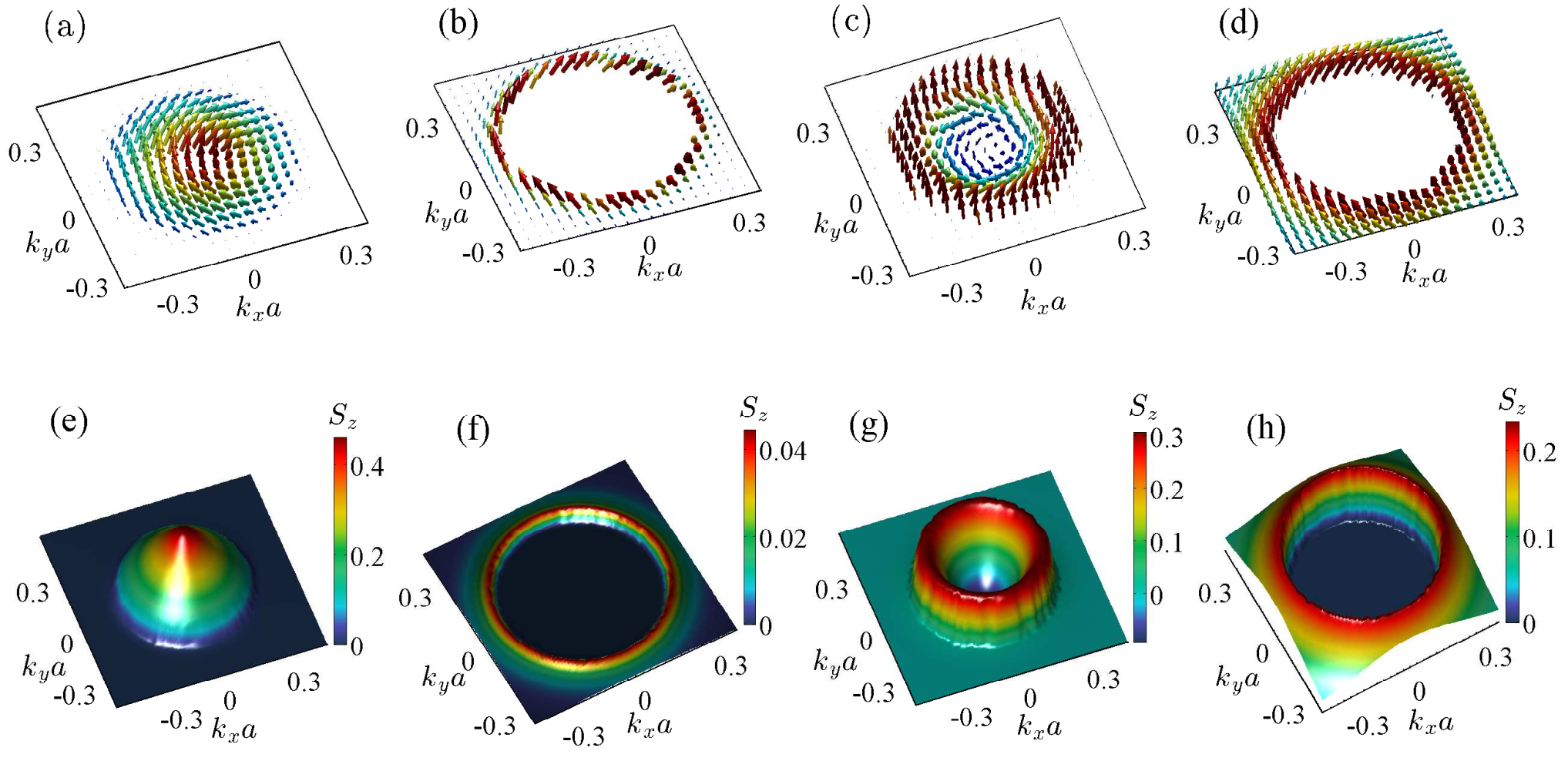
In the absence of the exchange field (i.e. with $h_{z}=0$), two degenerate Dirac cones appear near the $\bar{\Gamma}$ point in the spectrum; the corresponding states are spatially confined to the top or the bottom surface. With the adopted set of parameters, the Dirac point is not precisely located at the zero energy, but it can be easily tuned using a chemical potential. Once the TRS is broken by a finite $h_{z}$, the two-fold degeneracy is lifted in all the bands and the surface state, which experiences the exchange field, acquires a gap. In Fig. 1, we plot the momentum-space “spin” texture $\mathbf{S}(\mathbf{k})$ and the $z$-component of the “spin” expectation value $S_{z}(\mathbf{k})$ projected into the surface layer (with $l_{z}=1$), which is subject to the exchange field, in the vicinity of the Dirac point in the 2D surface Brillouin zone. $\mathbf{S}(\mathbf{k})$ is evaluated as the sum of the $l_{z}=1$ contributions from the two surface-centered bands, top and bottom (marked in red and green in Figs. 3(a) and 3(b)). The resultant of the two bands is taken here, because the surface bands hybridize away from the Brillouin zone center (see below and the Supplemental Materials). The “spin” texture in the selected surface layer changes qualitatively upon increasing the exchange field. The texture in Fig. 1(a) for $h_{z}=0.1~$eV is “hedgehog”-like. A similar pattern was detected in the spin-resolved ARPES experiments on Mn doped Bi₂Se₃ [23]. For larger field strength, the momentum-space “spin” structure transforms into a skyrmion-like texture as shown in Fig. 1(c). Most noticeable is the sign change of $S_{z}$ in the near vicinity of the surface Brillouin zone center, the $\bar{\Gamma}$ point ($|\mathbf{k}|=0$). Increasing $h_{z}$ further leads to yet another qualitative change of the “spin” texture. At first sight, the texture in Fig. 1(d) appears to have changed only quantitatively in comparison with Fig. 1(c). But as the analysis below will reveal, the topological character of these textures is indeed qualitatively different.

In order to decisively identify the topological character of the “spin” textures in Fig. 1, we calculate the skyrmion number $N=\frac{1}{4\pi}\int d\mathbf{k}~\tilde{\mathbf{S}}\cdot(\frac{\partial\tilde{\mathbf{S}}}{\partial k_{x}}\times\frac{\partial\tilde{\mathbf{S}}}{\partial k_{y}})$ in the exchange-split occupied surface band (the green band in Fig. 3(c)) at the top surface ($l_{z}=1$) of the slab, where the integral is extended to the hexagonal surface Brillouin zone. $\tilde{\mathbf{S}}$ is the normalized “spin” expectation value which ensures the quantization of the skyrmion number. $N$ as a function of the exchange field strength $h_{z}$ is shown in Fig. 2(a). Indeed, $N=1/2$ for exchange fields below the critical value $h_{zc1}=0.273$ eV, identifying more precisely that the hedgehog phase has the “spin” texture of a half-skyrmion (or meron). At $h_{zc1}$, the skyrmion number switches to $-1$, indicating the (anti)-skyrmion character of the texture for $h_{zc1}<h_{z}\leqslant h_{zc2}=0.31$ eV, and $N=0$ beyond $h_{zc2}$. The discontinuous changes of $N$ decisively display the signals for topological phase transitions. $N$ takes a finite value ($1/2$ or $-1$) in the exchange-split surface band (green band in Fig. 3(a)–(c)) only and is zero in the unsplit surface band (red band in Fig. 3(a)–(c)). Two types of skyrmion lattices commonly appear in chiral magnets. They are either classified as N$\acute{e}$el-type or Bloch-type skyrmion (see e.g. [35, 36, 37]); both have the same skyrmion number, but they differ in their spin-winding pattern. A closer inspection of Fig. 1(a) reveals that the momentum-space texture emerging here is a Bloch-type skyrmion.

The characteristic “spin” texture in the exchange-split surface band in the surface layer with finite $h_{z}$ is particularly evident within a circular region around the $\bar{\Gamma}$ point. Characteristic momentum-space radii $R_{H}$ and $R_{S}$ can be determined at which the polar angle $\Theta=\cos^{-1}{\{S_{z}/|\mathbf{S}|\}}$ of the “spins” has changed by $90^{\circ}$ or $180^{\circ}$ for the hedgehog and the skyrmion pattern, respectively, upon moving radially outward from the $\bar{\Gamma}$ point. Figure 2(b) shows the variation of $S_{z}$ in the occupied part of the exchange-split surface band with respect to $R_{\mathbf{k}}=\sqrt{k_{x}^{2}+k_{y}^{2}}$ and thereby identifies the special radius $R_{\mathbf{k}s}\simeq 0.3/a$ inside which the characteristic hedgehog and skyrmion textures form. At $R_{\mathbf{k}s}$, $|\mathbf{S}(\mathbf{k})|$ sharply drops to nearly zero. $\mathbf{S}(\mathbf{k})$ in the unsplit surface band has a complementary pattern beyond $R_{\mathbf{k}s}$ (see Supplemental Materials, Fig. S1). As discussed above (see also Fig. 2(b)), $S_{z}(\bar{\Gamma})$ changes sign at the critical field $h_{zc1}$.

As illustrated in Fig. 2(c), the polar angle $\Theta$, calculated in the occupied part of the exchange-split surface band, continuously varies from $\Theta=0^{\circ}$ at $R_{\mathbf{k}}=0$ to $\Theta=90^{\circ}$ at $R_{\mathbf{k}}=R_{H}$ for the hedgehog texture, and from $\Theta=180^{\circ}$ at $R_{\mathbf{k}}=0$ to $\Theta=0^{\circ}$ at $R_{\mathbf{k}}=R_{S}$ for the skyrmion texture. The plateaus, appearing at $\Theta=180^{\circ}$ and $\Theta=0^{\circ}$ for the skyrmion-“spin” texture, establish a distinctive difference to the typical spatial structure of skyrmions in chiral magnets [37]. With increasing $h_{z}$, the characteristic radius $R_{H}$ for the hedgehog texture increases slowly within the field range $0<h_{z}<h_{zc1}$, while the radius $R_{S}$ for the skyrmion texture increases rapidly within the field range $h_{zc1}<h_{z}\leqslant h_{zc2}$ as shown in Fig. 2(d). $R_{H}$ and $R_{S}$ even exceed further out than the special radius $R_{\mathbf{k}s}$. Beyond $h_{zc2}$, $\Theta$ stops at a finite angle and the “spins” no longer sweep to the opposite direction indicating the loss of the texture’s skyrmion character.

To get more insight into the origin of the topological phase transition, we analyze the changes in the electronic structure across the transition. In Figs. 3(a) and 3(b), the band dispersions of the slab are plotted in the hedgehog phase ($h_{z}=0.2~$eV) and at the critical field $h_{zc1}=0.273~$eV, respectively, along the $\bar{K}\rightarrow\bar{\Gamma}\rightarrow\bar{M}$ direction in the hexagonal surface Brillouin zone. Upon increasing $h_{z}$, the top occupied bulk band (orange) rises up in energy and touches the exchange-split surface band (green) at the $\bar{\Gamma}$ point for $h_{z}=h_{zc1}$, as depicted in Fig. 3(b). The former turns back towards the lower-energy bulk bands upon further increasing $h_{z}$.

The exchange-split and unsplit surface bands have an avoided level crossing at $R_{\mathbf{k}s}\simeq 0.3/a$, as visible in Fig. 3(c). This observation clarifies the role of the special radius $R_{\mathbf{k}s}$ within which the hedgehog and skyrmion textures form. The hybridization between the two (top and bottom) surface bands of the slab is possible, because their corresponding wave functions extend towards the interior of the slab at momenta away from the $\bar{\Gamma}$ point and therefore allow for a finite overlap (see also the Supplemental Materials).

Fig. 3(d) shows the variation of the energy gap at the $\bar{\Gamma}$ point of the exchange-split surface band and the gap between the occupied part of this band and the top occupied bulk band. When the exchange field reaches $h_{z}=h_{zc1}$, a bulk and a surface states become degenerate at the $\bar{\Gamma}$ point. Figures 3(e) and 3(f) show the squared amplitude of the wave functions at the $\Psi_{\bar{\Gamma}}$, calculated for the occupied exchange-split surface band and the top occupied bulk band, as a function of the layer index $l_{z}$ for $h_{z}=0.2~$eV (hedgehog phase) and $h_{z}=0.3~$eV (skyrmion phase). Evidently, these states interchange their spatial character across the transition.

An experimental detection of the skyrmion texture will be challenging using spin-resolved ARPES techniques. The real obstacle, however, to induce the topological transition is the required large exchange splitting. For the Bi₂Se₃ specific parameter set which we have used in our calculations, the required exchange field is more than four times larger than the so far observed splitting of $\sim 50~$meV in Bi₂Se₃ samples which are homogeneously doped with magnetic impurities [24]. At the TI/MI heterointerface of Bi₂Se₃/MnSe(111), the exchange splitting is only $7$ meV [46]. Yet, the extraordinarily large g-factor of $\sim$50 observed for the Dirac electrons in the Bi₂Se₃ surface states may render it possible to achieve unusually large exchange splittings [47, 25]. We have verified that the critical field can be reduced by applying an electric field along $z$-direction (up to $\sim$15$\%$ by a bias voltage of $0.1~$V between the two open surfaces). The phenomenon of the topological transition is expected to be generic to other strong TIs as well. Therefore, the selection of a TI with a band gap, narrower than Bi₂Se₃, is another possible route to realize the anticipated topological transition or the “spin”-skyrmion texture in momentum space itself.

The encountered topological phase transition provides a new example where the energy gap at the Fermi level does not close across the transition. Remarkably, while the skyrmion counting number changes, the Hall conductance remains constant. The hedgehog to skyrmion phase transition in the momentum-space “spin” texture is yet another striking phenomenon to occur in three dimensional topological insulators.

The authors gratefully acknowledge discussions with Daniel Braak. This work was supported by the DFG through TRR 80.

Supplemental Materials: Emergent Momentum-Space Skyrmion Texture on the Surface of Topological Insulators

References

- [1] L. Fu, C. L. Kane, and E. J. Mele, Phys. Rev. Lett. 98, 106803 (2007).
- [2] L. Fu and C. L. Kane, Phys. Rev. B 76, 045302 (2007).
- [3] M. Z. Hasan and C. L. Kane, Rev. Mod. Phys. 82, 3045 (2010).
- [4] J. E. Moore, Nature 464, 194 (2010).
- [5] R. Yu, W. Zhang, H.-J. Zhang, S.-C. Zhang, X. Dai, and Z. Fang, Science 329, 61 (2010).
- [6] C.-Z. Chang, J. Zhang, X. Feng, J. Shen, Z. Zhang, M. Guo, K. Li, Y. Ou, P. Wei, L.-L. Wang, Z.-Q. Ji, Y. Feng, S. Ji, X. Chen, J. Jia, X. Dai, Z. Fang, S.-C. Zhang, K. He, Y. Wang, L. Lu, X.-C. Ma, and Q.-K. Xue, Science 340, 167 (2013).
- [7] X. Kou, S.-T. Guo, Y. Fan, L. Pan, M. Lang, Y. Jiang, Q. Shao, T. Nie, K. Murata, J. Tang, Y. Wang, L. He, T.-K. Lee, W.-L. Lee, and K. L. Wang, Phys. Rev. Lett. 113, 137201 (2014).
- [8] J. Wang, B. Lian, and S.-C. Zhang, Phys. Scripta 2015, 014003 (2015).
- [9] H. Jiang, Z. Qiao, H. Liu, and Q. Niu, Phys. Rev. B 85, 045445 (2012).
- [10] L. Q. Duong, H. Lin, W.-F. Tsai, and Y. P. Feng, Phys. Rev. B 92, 115205 (2015).
- [11] I. Garate and M. Franz, Phys. Rev. Lett. 104, 146802 (2010).
- [12] R. Li, J. Wang, X.-L. Qi, and S.-C. Zhang, Nat. Phys. 6, 284 (2010).
- [13] A. M. Essin, J. E. Moore, and D. Vanderbilt, Phys. Rev. Lett. 102, 146805 (2009).
- [14] X.-L. Qi, T. L. Hughes, and S.-C. Zhang, Phys. Rev. B 78, 195424 (2008).
- [15] H. Zhang, C.-X. Liu, X.-L. Qi, X. Dai, Z. Fang, and S.-C. Zhang, Nat. Phys. 5, 438 (2009).
- [16] O. V. Yazyev, J. E. Moore, and S. G. Louie, Phys. Rev. Lett. 105, 266806 (2010).
- [17] X.-L. Qi and S.-C. Zhang, Rev. Mod. Phys. 83, 1057 (2011).
- [18] H. Zhang, C.-X. Liu, and S.-C. Zhang, Phys. Rev. Lett. 111, 066801 (2013).
- [19] D. Hsieh, Y. Xia, L. Wray, D. Qian, A. Pal, J. H. Dil, J. Osterwalder, F. Meier, G. Bihlmayer, C. L. Kane, Y. S. Hor, R. J. Cava, and M. Z. Hasan, Science 323, 919 (2009).
- [20] S. Souma, K. Kosaka, T. Sato, M. Komatsu, A. Takayama, T. Takahashi, M. Kriener, K. Segawa, and Y. Ando, Phys. Rev. Lett. 106, 216803 (2011).
- [21] Z.-H. Pan, E. Vescovo, A. V. Fedorov, D. Gardner, Y. S. Lee, S. Chu, G. D. Gu, and T. Valla, Phys. Rev. Lett. 106, 257004 (2011).
- [22] C. Jozwiak, Y. L. Chen, A. V. Fedorov, J. G. Analytis, C. R. Rotundu, A. K. Schmid, J. D. Denlinger, Y.-D. Chuang, D.-H. Lee, I. R. Fisher, R. J. Birgeneau, Z.-X. Shen, Z. Hussain, and A. Lanzara, Phys. Rev. B 84, 165113 (2011).
- [23] S.-Y. Xu, M. Neupane, C. Liu, D. Zhang, A. Richardella, L. Andrew Wray, N. Alidoust, M. Leandersson, T. Balasubramanian, J. Sanchez-Barriga, O. Rader, G. Landolt, B. Slomski, J. Hugo Dil, J. Osterwalder, T.-R. Chang, H.-T. Jeng, H. Lin, A. Bansil, N. Samarth, and M.-Z. Hasan, Nat. Phys. 8, 616 (2012).
- [24] Y. L. Chen, J.-H. Chu, J. G. Analytis, Z. K. Liu, K. Igarashi, H.-H. Kuo, X. L. Qi, S. K. Mo, R. G. Moore, D. H. Lu, M. Hashimoto, T. Sasagawa, S. C. Zhang, I. R. Fisher, Z. Hussain, and Z. X. Shen, Science 329, 659 (2010).
- [25] P. Wei, F. Katmis, B. A. Assaf, H. Steinberg, P. Jarillo-Herrero, D. Heiman, and J. S. Moodera, Phys. Rev. Lett. 110, 186807 (2013).
- [26] M. Lang, M. Montazeri, M. C. Onbasli, X. Kou, Y. Fan, P. Upadhyaya, K. Yao, F. Liu, Y. Jiang, W. Jiang, K. L. Wong, G. Yu, J. Tang, T. Nie, L. He, R. N. Schwartz, Y. Wang, C. A. Ross, and K. L. Wang, Nano Lett. 14, 3459 (2014).
- [27] A. J. Bestwick, E. J. Fox, X. Kou, L. Pan, K.-L. Wang, and D. Goldhaber-Gordon, Phys. Rev. Lett. 114, 187201 (2015).
- [28] A. Bauer and C. Pfleiderer, Phys. Rev. B 85, 214418 (2012).
- [29] C.-X. Liu, X.-L. Qi, H. Zhang, X. Dai, Z. Fang, and S.-C. Zhang, Phys. Rev. B 82, 045122 (2010).
- [30] P. Larson, V. A. Greanya, W. C. Tonjes, R. Liu, S. D. Mahanti, and C. G. Olson, Phys. Rev. B 65, 085108 (2002).
- [31] A. Pertsova and C. M. Canali, New J. Phys. 16, 063022 (2014).
- [32] Y. Xia, D. Qian, D. Hsieh, L. Wray, A. Pal, H. Lin, A. Bansil, D. Grauer, Y. S. Hor, R. J. Cava, and M. Z. Hasan, Nat. Phys. 5, 398 (2009).
- [33] D. Hsieh, Y. Xia, D. Qian, L. Wray, J. H. Dil, F. Meier, J. Osterwalder, L. Patthey, J. G. Checkelsky, N. P. Ong, A. V. Fedorov, H. Lin, A. Bansil, D. Grauer, Y. S. Hor, R. J. Cava, and M. Z. Hasan, Nature 460, 1101 (2009).
- [34] K. Ebihara, K. Yada, A. Yamakage, and Y. Tanaka, Physica E 44, 885 (2012).
- [35] U. K. Roszler, A. N. Bogdanov, and C. Pfleiderer, Nature 442, 797 (2006).
- [36] I. Kezsmarki, S. Bordacs, P. Milde, E. Neuber, L. M. Eng, J. S. White, H. M. Ronnow, C. D. Dewhurst, M. Mochizuki, K. Yanai, H. Nakamura, D. Ehlers, V. Tsurkan, and A. Loidl, Nat. Mater. 14, 1116 (2015).
- [37] N. Nagaosa and Y. Tokura, Nat. Nano. 8, 899 (2013).
- [38] M. Onoda, G. Tatara, and N. Nagaosa, J. Phys. Soc. Jpn. 73, 2624 (2004).
- [39] M. Kohmoto, Ann. Phys. 160, 343 (1985).
- [40] J. Linder, T. Yokoyama, and A. Sudbø, Phys. Rev. B 80, 20540 (2009).
- [41] Y. Zhang, K. He, C.-Z. Chang, C.-L. Song, L.-L. Wang, X. Chen, J.-F. Jia, Z. Fang, X. Dai, W.-Y. Shan, S.-Q. Shen, Q. Niu, X.-L. Qi, S.-C. Zhang, X.-C. Ma, and Q.-K. Xue, Nat. Phys. 6, 584 (2010).
- [42] Y. Sakamoto, T. Hirahara, H. Miyazaki, S.-I. Kimura, and S. Hasegawa, Phys. Rev. B 81, 165432 (2010).
- [43] C.-X. Liu, H.-J. Zhang, B. Yan, X.-L. Qi, T. Frauenheim, X. Dai, Z. Fang, and S.-C. Zhang, Phys. Rev. B 81, 041307 (2010).
- [44] H. Ozawa, A. Yamakage, M. Sato, and Y. Tanaka, Phys. Rev. B 90, 045309 (2014)
- [45] M. Ezawa, Y. Tanaka, and N. Nagaosa, Sci. Rep. 3, 2790 (2013).
- [46] S. V. Eremeev, V. N. Men’shov, V. V. Tugushev, P. M. Echenique, and E. V. Chulkov, Phys. Rev. B 88, 144430 (2013).
- [47] J. G. Analytis, R. D. McDonald, S. C. Riggs, J.-H. Chu, G. S. Boebinger, and I. R. Fisher, Nat. Phys. 6, 960 (2010).
- [48] M. Li, C.-Z. Chang, B. J. Kirby, M. E. Jamer, W. Cui, L. Wu, P. Wei, Y. Zhu, D. Heiman, J. Li, and J. S. Moodera, Phys. Rev. Lett. 115, 087201 (2015).
- [1] K. Ebihara, K. Yada, A. Yamakage, and Y. Tanaka, Physica E 44, 885 (2012).
- [2] C.-X. Liu, X.-L. Qi, H. Zhang, X. Dai, Z. Fang, and S.-C. Zhang, Phys. Rev. B 82, 045122 (2010).
- [3] J. Linder, T. Yokoyama, and A. Sudbø, Phys. Rev. B 80, 20540 (2009).
- [4] Y. Zhang, K. He, C.-Z. Chang, C.-L. Song, L.-L. Wang, X. Chen, J.-F. Jia, Z. Fang, X. Dai, W.-Y. Shan, S.-Q. Shen, Q. Niu, X.-L. Qi, S.-C. Zhang, X.-C. Ma, and Q.-K. Xue, Nat. Phys. 6, 584 (2010).
- [5] Y. Sakamoto, T. Hirahara, H. Miyazaki, S.-I. Kimura, and S. Hasegawa, Phys. Rev. B 81, 165432 (2010).
- [6] C.-X. Liu, H.-J. Zhang, B. Yan, X.-L. Qi, T. Frauenheim, X. Dai, Z. Fang, and S.-C. Zhang, Phys. Rev. B 81, 041307 (2010).
- [7] H. Ozawa, A. Yamakage, M. Sato, and Y. Tanaka, Phys. Rev. B 90, 045309 (2014)