Carbon-oxygen-neon mass nuclei in superstrong magnetic fields

We consider a nucleus in a magnetic field which is described by the Hamilton operator $\hat{h}_{q}=\hat{h}^{(0)}_{q}+\hat{h}^{(B)}_{q}$, where $q\in\{p,n\}$ specifies the isospin of a nucleon and $\hat{h}^{(0)}_{q}$ is the Hamiltonian in the absence of a $B$ field, which is given by Eq. (8) of Ref. [13]. It is constructed in terms of densities and currents of nucleons. The term $\hat{h}^{(B)}_{q}$ which is due to the $B$ field is given by

where $\tilde{{\bm{B}}_{q}}\equiv({e\hbar}/{2\,m_{q}c}){\bm{B}}\,,$ ${\bm{\sigma}}$ is the spin Pauli matrix, and ${\bm{l}}$ is the (dimensionless) orbital angular momentum. These are related to the spin ${\bm{S}}$ and the orbital angular momentum ${\bm{L}}$ via ${\bm{S}}=\hbar{\bm{\sigma}}/2$ and ${\bm{L}}=\hbar{\bm{l}}$, where $g_{n}=-3.826$ and $g_{p}=5.585$ are the $g$ factors of neutrons and protons. The Kronecker-delta takes into account the fact that neutrons do not couple with their orbital angular momenta.

Starting from the Hamiltonian $\hat{h}_{q}$ one can construct the density functional (DF) in the basis Hartree-Fock wave functions. We use the DF which contains the kinetic energy, the nuclear Skyrme interaction, the Coulomb energy, and the correlation correction to the mean-field DF. In principle the pairing correction can be added to the DF, but we ignore it here because of its overall smallness and because the $S$-wave pairing would be quenched by the magnetic field [14]. The correlation correction in the DF includes those corrections which reflect the beyond-mean-field contributions.

We have used the code SKY3D to find iteratively the solution of the static HF equation in strong magnetic fields. The equations are solved using successive approximations to the wave functions on a three-dimensional Cartesian grid, which has 32 points along each direction and a distance between the points of 1.0 fm. (We varied the parameters of the mesh within reasonable values and made sure that the physical results are unchanged). To accelerate the iteration a damping of the kinetic term is performed. The following ranges of the two numerical parameters of the damped gradient step have been used - the step size $\delta=0.4$ and the damping regulator $E_{0}=100$ MeV. After performing a wave-function iteration steps, the densities of the nucleons are updated and new mean fields are computed. This provides the starting point for the next iteration. The iterations are continued until convergence to the desired accuracy is achieved. As a convergence criterion the average energy variance or the fluctuation of single-particle states is used. To initialize the problem we use harmonic oscillator states and include an unoccupied nucleon state. The radii of the harmonic oscillator states are $r_{\rm h.o.}\simeq 3$ fm. Our computations were carried out with the SV-bas version of the Skyrme force [15]. The magnetic field direction was chosen along the $z$ direction, but other directions were also tested to produce identical results. Initially nuclei with $B=0$ were computed, thereafter the magnetic field was incremented with steps of about 0.25$\sqrt{\textrm{MeV}~\textrm{fm}^{-3}}$ as long as the convergence was achieved for the number of iterations $N_{i}\leq 4000$. The direction of the $B$ field was chosen always as the $z$ axis of Cartesian coordinates, unless stated otherwise.

To access the shape and size of the nuclei we examined the radii $r_{\mathrm{rms}}$, the total deformation $\beta$ and the triaxiality $\gamma$ (for definitions see, e. g., [16]). Here $\gamma=0\degree$ refers to a prolate deformed nucleus, $\gamma=60\degree$ refers to an oblate deformed nucleus, and angles between $\gamma=0\degree$ and $\gamma=60\degree$ refer to a deformation in a state between prolate and oblate. If $\beta=0$ the nucleus is spherical (undeformed) independent of $\gamma$. For non-zero $\beta$, the nuclei are deformed.

Before discussing the numerical results we provide approximate analytical formulas for energy level splitting and $z$ components of angular momentum and spin in terms of Clebsch-Gordan coefficients. We adopt the definition of the Clebsch-Gordan coefficients [16]:

where $l$ is the orbital angular momentum, $s$ the spin, and $J$ the total angular momentum and $m_{l}$, $m_{s}$, and $M$ are the $z$ components of $l$, $s$, and $J$, respectively. The following conditions need to be fulfilled:

For nucleons $s=1/2$ always and, therefore, $m_{s}=\pm 1/2$, $l$ is a non-negative integer number, and $m_{l}$ is an integer number, which can be positive, negative, or zero. Thus, $J$ assumes non-negative half-integer numbers; $M$ assumes half-integer numbers, which can be positive or negative. Writing out formula (2) for the lowest states of a nucleus and inserting the values of the Clebsch-Gordan coefficients we find for the $s$ states

where on both side of these equations we omitted the trivial value of spin $s=1/2$ appearing in Eq. (2). For the $p$ states we find

The states can be divided into mixed states that are linear combinations of certain $\left|lm_{l}sm_{s}\right>$ states and pure states which involve only one set of these quantum numbers. The energy levels of spin-up and -down particles are split in a magnetic field. This splitting is given by

which can be expressed in terms of the Clebsch-Gordan coefficients

The $z$-components of the angular momentum and spin can be as well expressed through the Clebsch-Gordan coefficients according to

Table 1 lists values of energy splitting, and $z$ components of angular momentum and spin according to Eqs. (7)-(9) for neutron and proton states. These analytical results can be compared to the results of the SKY3D code, to which we now turn.

The states of protons and neutrons in ${{}^{\makebox[7.97226pt][r]{$\scriptstyle 16$}}_{\makebox[7.97226pt][r]{$\scriptstyle$}}\mathrm{O}}$ nucleus are shown in Figs. 1 and 2 as a function of the magnetic field. For the fields $B\geq 10^{16}\,$G the split in the energy levels of spin-up and spin-down states becomes sizable (of the order of the nuclear scale MeV). For the $s$ states the splitting increases linearly with the magnitude of magnetic field. For $p$ states this dependence is more complicated. Below the critical field $B_{c}[{{}^{\makebox[7.97226pt][r]{$\scriptstyle 16$}}_{\makebox[7.97226pt][r]{$\scriptstyle$}}\mathrm{O}}]=4.0\times 10^{17}\,$G, the filling of the states corresponds to that of the lowest available states of the harmonic oscillator. However, for fields larger than $B_{c}[{{}^{\makebox[7.97226pt][r]{$\scriptstyle 16$}}_{\makebox[7.97226pt][r]{$\scriptstyle$}}\mathrm{O}}]\,$ the occupation pattern for protons changes: the $d_{5/2},M=+5/2$ state becomes occupied instead of the $p_{1/2},M=-1/2$ state (which is not shown above this field value) in Fig. 1. We also find that above the critical field $B_{c}[{{}^{\makebox[7.97226pt][r]{$\scriptstyle 16$}}_{\makebox[7.97226pt][r]{$\scriptstyle$}}\mathrm{O}}]$ the energy levels undergo an abrupt rearrangement. For the pure states (all $s$ states and $p$ states with $M=\pm 3/2)$, we obtain a good agreement between the numerical and analytical results for the energy levels. For the mixed states the discrepancy between the numerical and analytical results is below 10$\%$ of the energy of the corresponding level. The computations of the energy levels for the ${{}^{\makebox[7.97226pt][r]{$\scriptstyle 12$}}_{\makebox[7.97226pt][r]{$\scriptstyle$}}\mathrm{C}}$ nucleus show the same basic features seen already in the case of ${{}^{\makebox[7.97226pt][r]{$\scriptstyle 16$}}_{\makebox[7.97226pt][r]{$\scriptstyle$}}\mathrm{O}}$, see Figs. 3 and 4. In this case the numerical and analytical differ by at most 10$\%$ of the energy of the levels, the discrepancy increasing with the field. The same applies to the case of the ${{}^{\makebox[7.97226pt][r]{$\scriptstyle 20$}}_{\makebox[7.97226pt][r]{$\scriptstyle$}}\mathrm{Ne}}$ nucleus, but classification of the levels in this case is more complex because apart from the $1s$ and $1p$ states two $1d_{5/2}$ states should be filled. This nucleus is deformed in the ground state and the axis of the deformation may not coincide with the direction of the magnetic field, in which case there are no states with half-integer values of $(\langle L_{z}\rangle+\langle S_{z}\rangle)/\hbar$. In addition to the energy levels, we have also computed the $z$ components of orbital angular momentum $\left<L_{z}\right>$ and spin $\left<S_{z}\right>$ of neutrons and protons as functions of the magnetic field. The results are shown in Figs. 1 and 2. For the $s$ states, defined in Eqs. (4a) and (4b), as well as pure $p$ states (5a) and (5d) we obtain integer or half integer numbers for $\left<L_{z}\right>/\hbar$ or $\left<S_{z}\right>/\hbar$ which are identical to the quantum numbers $m_{l}$ or $m_{s}$, respectively, are independent of the magnetic field, and therefore are not shown in Figs. 1 and 2.

For mixed states given by Eqs. (5b), (5c), (5e) and (5f), $\left<L_{z}\right>$ and $\left<S_{z}\right>$ change as functions of the magnetic field as seen from these figures. For these states at any magnetic field $M=m_{l}+m_{s}=(\left<L_{z}\right>+\left<S_{z}\right>)/\hbar$ is a good quantum number. In the limit of weak magnetic fields the angular momentum and spin are coupled via the l-s coupling. Then $\left<L_{z}\right>$ and $\left<S_{z}\right>$ for each state are given according to Table 1. Because of the l-s coupling the vectors of ${\bm{L}}$ and ${\bm{S}}$ are not aligned with the magnetic field separately. The influence of the weak magnetic field on the system is described by the Zeeman effect. In the regime of strong magnetic fields the l-s coupling is ineffective, i.e., the orbital angular momentum $l$ and the spin $s$ couple separately to the magnetic field. In this case, the mixed states reach asymptotically the following non mixed states:

Thus we observe a smooth transition from the l-s to the separate l-B and s-B coupling as the magnetic field is increased, which can be viewed as a transition from the Zeeman to the Paschen-Back effect. Finally we note that for the $d_{5/2}(M=+5/2)$ state $\left<L_{z}\right>/\hbar=m_{l}=2$ and $\left<S_{z}\right>/\hbar=m_{s}=1/2$ assume constant values for all magnetic fields and are therefore not shown in Fig. 1. The key features observed for components $\left<L_{z}\right>$ and $\left<S_{z}\right>$ of ${{}^{\makebox[7.97226pt][r]{$\scriptstyle 16$}}_{\makebox[7.97226pt][r]{$\scriptstyle$}}\mathrm{O}}$ persist in the case of ${{}^{\makebox[7.97226pt][r]{$\scriptstyle 12$}}_{\makebox[7.97226pt][r]{$\scriptstyle$}}\mathrm{C}}$ and we do not show them here.

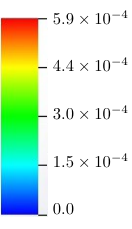
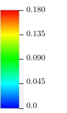
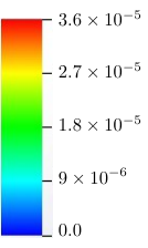
We have extracted the current and spin densities as a functions of the magnetic field for the ${{}^{\makebox[7.97226pt][r]{$\scriptstyle 12$}}_{\makebox[7.97226pt][r]{$\scriptstyle$}}\mathrm{C}}$, ${{}^{\makebox[7.97226pt][r]{$\scriptstyle 16$}}_{\makebox[7.97226pt][r]{$\scriptstyle$}}\mathrm{O}}$, and ${{}^{\makebox[7.97226pt][r]{$\scriptstyle 20$}}_{\makebox[7.97226pt][r]{$\scriptstyle$}}\mathrm{N}}$ nuclei. It is more convenient to show the collective flow velocity instead of the currents by dividing these with the particle density. The velocity distribution in ${{}^{\makebox[7.97226pt][r]{$\scriptstyle 16$}}_{\makebox[7.97226pt][r]{$\scriptstyle$}}\mathrm{O}}$ is shown in Fig. 5. The top and middle panels compare the velocity distribution for neutrons and protons for the field $B=3.9\times 10^{17}\,$G; the background shows the density distribution within the nucleus. It is seen that the magnitude of the proton current is by a factor of 4 larger than the neutron current. We also observe that the proton and neutron currents are counter-moving and concentrated around the surface of the nucleus. Note that the current density is shown in the plane orthogonal to the field. In the case of ${{}^{\makebox[7.97226pt][r]{$\scriptstyle 12$}}_{\makebox[7.97226pt][r]{$\scriptstyle$}}\mathrm{C}}$ we find current patterns of neutrons and protons similar to those seen in ${{}^{\makebox[7.97226pt][r]{$\scriptstyle 16$}}_{\makebox[7.97226pt][r]{$\scriptstyle$}}\mathrm{O}}$. The currents are counter-moving for neutrons and protons, their magnitudes increase with the field value and are mostly concentrated at the surface of the nuclei. Because there is no rearrangement seen for ${{}^{\makebox[7.97226pt][r]{$\scriptstyle 12$}}_{\makebox[7.97226pt][r]{$\scriptstyle$}}\mathrm{C}}$ this increase, in contrast to ${{}^{\makebox[7.97226pt][r]{$\scriptstyle 16$}}_{\makebox[7.97226pt][r]{$\scriptstyle$}}\mathrm{O}}$, is gradual. The velocities of protons in ${}^{\makebox[7.97226pt][r]{$\scriptstyle 20$}}_{\makebox[7.97226pt][r]{$\scriptstyle$}}\mathrm{Ne}$ are shown in Fig. 6 for two magnetic fields $B=4.0\times 10^{13}\,$G and the maximal studied field $B=4.9\times 10^{17}\,$G. The four orders of magnitude increase in the field leads to an increase in the maximal current by about the same factor. The current is concentrated at the surface of the field; note that the magnetic field induces a change in the shape of the nucleus (density distribution) which in turn affects the pattern of currents, which are more circular for a larger magnetic field.

We consider now the spin density of neutrons and protons in the nuclei under consideration and the effect of the spin interaction with the magnetic field. The spin-density for ${}^{\makebox[7.97226pt][r]{$\scriptstyle 16$}}_{\makebox[7.97226pt][r]{$\scriptstyle$}}\mathrm{O}$ is shown in Fig. 7. The spins of neutrons and protons are anti-parallel as expected from Eq. (1). In the case of ${}^{\makebox[7.97226pt][r]{$\scriptstyle 16$}}_{\makebox[7.97226pt][r]{$\scriptstyle$}}\mathrm{O}$ the spin polarization increases abruptly for protons because of the rearrangement of the levels. For weak magnetic fields the l-s coupling is dominant therefore the alignment of the spins is not pronounced; for strong magnetic fields the spins are aligned with the $z$-axis. We find that in the case of ${}^{\makebox[7.97226pt][r]{$\scriptstyle 12$}}_{\makebox[7.97226pt][r]{$\scriptstyle$}}\mathrm{C}$ the spin alignment is more pronounced than for ${}^{\makebox[7.97226pt][r]{$\scriptstyle 16$}}_{\makebox[7.97226pt][r]{$\scriptstyle$}}\mathrm{O}$, i.e., ${}^{\makebox[7.97226pt][r]{$\scriptstyle 12$}}_{\makebox[7.97226pt][r]{$\scriptstyle$}}\mathrm{C}$ is more polarizable. In Fig. 8 we show the spin polarization in the ${}^{\makebox[7.97226pt][r]{$\scriptstyle 20$}}_{\makebox[7.97226pt][r]{$\scriptstyle$}}\mathrm{Ne}$ nucleus, where the new feature is the deformation of the nucleus in the ground state in the absence of a magnetic field. For small magnetic fields a clear evidence of two symmetry axes is present. For larger magnetic fields the spin polarization by the magnetic field directs the spin alongs the field axis ($z$ direction). We note that in all cases protons and neutron show quantitatively similar polarization (the minor difference coming from different values of their $g$ factors).

Finally, we want to consider the shape and the size of the ${}^{\makebox[7.97226pt][r]{$\scriptstyle 16$}}_{\makebox[7.97226pt][r]{$\scriptstyle$}}\mathrm{O}$ nucleus for non-zero magnetic fields. For $B<B_{c}[{{}^{\makebox[7.97226pt][r]{$\scriptstyle 16$}}_{\makebox[7.97226pt][r]{$\scriptstyle$}}\mathrm{O}}]\,$, the lowest states of the harmonic oscillator are filled and the shape of the nucleus is spherical. Its radius is $r_{\mathrm{rms}}=2.69\,$fm. For $B>B_{c}[{{}^{\makebox[7.97226pt][r]{$\scriptstyle 16$}}_{\makebox[7.97226pt][r]{$\scriptstyle$}}\mathrm{O}}]\,$ the nucleus is deformed with deformation parameters $\beta=0.1$ and $\gamma=60\degree$, which implies that the deformation is oblate. The mean radius is $r_{\mathrm{rms}}=2.72\,$fm in this case. The redistribution of neutron and proton states above the critical field has the effect of slightly deforming the nucleus from its spherical shape. We stress that the redistribution is found to be abrupt and therefore the change in the shape of the nucleus is abrupt as well.

In the case of the ${}^{\makebox[7.97226pt][r]{$\scriptstyle 12$}}_{\makebox[7.97226pt][r]{$\scriptstyle$}}\mathrm{C}$ nucleus we find that the shape of the nucleus does not change much with increasing magnetic field. For a zero field it is spherical symmetric with $r_{\mathrm{rms}}=2.47\,$fm, increasing slightly to 2.51 fm for $B_{c}=4.1\times 10^{17}\,$G. Increasing the magnetic field also results in a smooth deformation from $\beta=0$ at $B=0$ to $\beta=0.071$ for $B_{c}$. The deformation is always oblate with $\gamma=60\degree$.

The deformation of the ${}^{\makebox[7.97226pt][r]{$\scriptstyle 20$}}_{\makebox[7.97226pt][r]{$\scriptstyle$}}\mathrm{Ne}$ nucleus with the magnetic field is continuous and in contrast to the other examples above, the nucleus is deformed for a vanishing magnetic field. We find that its radius $r_{\mathrm{rms}}$ slightly decreases from 2.93 fm to 2.87 fm with the magnetic field. However, the $\beta$ parameter decreases from 0.32 to 0.15, i.e., to a value which is less than half of the original one. This is the only example of a continuous significant change in deformation as a function of magnetic field. The parameter $\gamma$ starts at $0\degree$ for $B=0$, but increases asymptotically to $11\degree$ implying a change from a purely prolate deformed nucleus to a mainly prolate deformed one. This evolution of ${}^{\makebox[7.97226pt][r]{$\scriptstyle 20$}}_{\makebox[7.97226pt][r]{$\scriptstyle$}}\mathrm{Ne}$ nucleus from deformed to the more spherical shape is visualized in Fig. 6.