Opinion Dynamics in Networks: Convergence, Stability and Lack of Explosion
Abstract
Inspired by the work of Kempe et al. [16], we introduce and analyze a model on opinion formation; the update rule of our dynamics is a simplified version of that of [16]. We assume that the population is partitioned into types whose interaction pattern is specified by a graph. Interaction leads to population mass moving from types of smaller mass to those of bigger. We show that starting uniformly at random over all population vectors on the simplex, our dynamics converges point-wise with probability one to an independent set. This settles an open problem of [16], as applicable to our dynamics. We believe that our techniques can be used to settle the open problem for the Kempe et al. dynamics as well.
Next, we extend the model of Kempe et al. by introducing the notion of birth and death of types, with the interaction graph evolving appropriately. Birth of types is determined by a Bernoulli process and types die when their population mass is less than a parameter . We show that if the births are infrequent, then there are long periods of “stability” in which there is no population mass that moves. Finally we show that even if births are frequent and “stability” is not attained, the total number of types does not explode: it remains logarithmic in .
1 Introduction
The birth, growth and death of political parties, organizations, social communities and product adoption groups (e.g., whether to use Windows, Mac OS or Linux) often follows common patterns, leading to the belief that the dynamics underlying these processes has much in common. Understanding this commonality is important for the purposes of predictability and hence has been the subject of study in mathematical social science for many years [4, 7, 8, 14, 27]. In recent years, the growth of social communities on the Internet, and their increasing economic and social value, has provided fresh impetus to this study [1, 2, 5, 18].
In this paper, we continue along these lines by building on a natural model proposed by Kempe et al. [16]. Their model consists of an influence graph on vertices (types, parties) into which the entire population mass is partitioned. Their main tenet is that individuals in smaller parties tend to get influenced by those in bigger parties 11 1 Changes in the sizes of political parties and other organizations can occur for a multitude of possible reasons, such as changes in economic conditions, immigration flows, wars and terrorism, and drastic changes in technology (such as the introduction of the Internet, smart phones and social media). Studying changes due to these multitude of reasons in a systematic quantitative manner is unrealistic. For this reason, many authors in computer science and the social sciences have limited their work to studying the effects of relative sizes of the groups, in itself a key factor, e.g. see [16]. Following these works, our paper also takes a similar approach.. Individuals in the two vertices connected by an edge can interact with each other. These interactions result in individuals moving from smaller to bigger in population vertices. Kempe et al. characterize stable equilibria of this dynamics via the notion of Lyapunov stability, and they show that under any stable equilibrium, the entire mass lies in an independent set, i.e., the population breaks into non-interacting islands. The message of this result is clear: a population is (Lyapunov) stable, in the sense that the system does not change by much under small perturbations, only if people of different opinions do not interact. They also showed convergence to a fixed point, not necessarily an independent set, starting from any initial population vector and influence graph. One of their main open problems was to determine whether starting uniformly at random over all population vectors on the unit simplex, their dynamics converge with probability one to an independent set.
We first settle this open problem in the affirmative for a modification of the dynamics, which however is similar as that of Kempe et al. in spirit in that it moves mass from smaller to bigger parties (the dynamics is defined below along with a justification). We believe that the ideas behind our analysis can be used to settle the open problem for the dynamics of Kempe et al. as well, via a more complicated spectral analysis of the Jacobian of the update rule of the dynamics (see Section 3.2).
Whereas the model of Kempe et al. captures and studies the effects of migration of individuals across types in a very satisfactory manner, it is quite limited in that it does not include the birth and death of types. In this paper, we model birth and death of types. In order to arrive at realistic definitions of these notions, we first conducted case studies of political parties in several countries. We present below a case study on Greek politics, but similar phenomena arise in India, Spain, Italy and Holland (see Wikipedia pages).
The Siriza party in Greece provides an excellent example of birth of a party (this information is readily available in Wikipedia pages). This party was essentially in a dormant state until the first 2012 elections in which it got 16.8% of the vote, mostly taken away from the Pasok party, which dropped from 43.9% to 13.2% in the process (Wikipedia). In the second election in 2012, Siriza increased its vote to 26.9% and Pasok dropped to 12.3%. Finally, in 2015, Siriza increased to 36.3% and Pasok dropped further to 4.7%. Another party, Potami, was formed in 2015 and got 6.1% of the vote, again mainly from Pasok. However, in a major 2016 poll, it seems to have collapsed and is likely be absorbed by other parties. In contrast, the KKE party in Greece, which had almost no interactions with the rest of the parties (and was like a disconnected component), has remained between 4.5-8.5% of the vote over the last 26 years.
Motivated by these examples, we have modeled birth and death of types in the following manner. We model population as a continuum, as is standard in population dynamics, and time is discrete. This is the same as arXiv Version 1 of [16], which is what we will refer to throughout this paper; the later versions study the continuous time analog. The birth of a new type in our model is determined by a Bernoulli process, with parameter . The newly born type absorbs mass from all other types via a randomized process given by an arbitrary distribution with finite support (see Section 2.2). After birth, the new type is connected to an arbitrary, though non-empty, set of other types. Our model has a parameter , and when the size of a type drops below , it simply dies, moving its mass equally among its neighbors.
Our rule for migration of mass, which is somewhat different from that of Kempe et al. is motivated by the following considerations. For a type , will denote the fraction of population that is of type . Assume that types and have an edge, i.e., their populations interact. If so, we will assume that some individuals of the smaller type get influenced by the larger one and move to the larger one. The question is what is a reasonable assumption on the population mass that moves.
For arriving at the rule proposed in this paper, consider three situations. If and , i.e., the smaller type is very small, then clearly not many people will move. If and , i.e., the types are approximately of the same population size, then again we expect not many people to move. Finally, if and , i.e., both types are reasonably big and their difference is also reasonably big, then we expect several people to move from the smaller to the bigger type. From these considerations, we propose that the amount of population mass moving from to , assuming , is given by the rule
where is a function that captures the level of influence between . We assume that is continuously differentiable, (there is no population flow between two neighboring types if they have the same fraction of population), is increasing and finally it is odd, i.e., (so that .
In this simplified setting we have made the assumption that the system is closed, i.e., that it does not get influence from outside factors (e.g., economical crisis, immigrations flows, terrorism etc).
1.1 Our results and techniques
We first study our migration dynamics without birth and death and settle the open problem of Kempe et al., as it applies to our dynamics. We show that the dynamics converges set-wise to a fixed point, i.e., there is a set containing only fixed points such that the distance between the trajectory of the dynamics and goes to zero for all starting population vectors. To show this convergence result, we use a simple potential function of the population mass namely, the norm of the population vector, and we show that this potential is strictly increasing at each time step (unless the dynamics is at a fixed point). Moreover, the potential is bounded, hence the result follows. Next, we strengthen this result by showing point-wise convergence as well. The latter result is technically deeper and more difficult, since it means that every trajectory converges to a specific fixed point . We show point-wise convergence by constructing a local potential function that is decreasing in a small neighborhood of the limit point . The potential function is always non-zero in that small neighborhood and is zero only at .
Using the latter result and one of the most important theorems in dynamical systems, the Center Stable Manifold Theorem, we prove that with probability one, under an initial population vector picked uniformly at random from the unit simplex, our dynamics converges point-wise to a fixed point , where the active types in , i.e., so that , form an independent set of . This involves characterization of the linearly stable (see Section 2.3 for definition) fixed points and proving that the update rule of the dynamics is a local diffeomorphism22 2 Continuously differentiable, the inverse exists and is also continuously differentiable.. This settles the open problem of Kempe et al., mentioned in the Introduction, for our dynamics. This result is important because it allows us to perform a long-term average case analysis of the behavior of our dynamics and make predictions.
Next, we introduce birth and death in our model. Clearly there will be no convergence in this case since new parties are created all the time. Instead we define and study a notion of “stability” which is different from the classical notions that appear in dynamical systems (see Section 2.3 for the definition of the classical notion and Definition 4.2 for our notion). A dynamics is -stable if and only if , no population mass moves at step . We show that despite birth and death, there are arbitrarily long periods of “stability” with high probability, for a sufficiently small . Finally, we show that in the long run, with high probability, for a sufficiently large , the number of types in the population will be . This may seem counter-intuitive, since with a large new types will be created often; however, since new types absorb mass from old types, the old types die frequently. In contrast, in the short term (from the definition of ) we can have up to types.
Let us give an interpretation of the results of the previous paragraph in terms of political parties of certain countries (information obtained from Wikipedia). Countries do have periods of political stability, e.g., during 1981-85, 2004-07, no new major (with more than 1% of the vote) parties were formed in Greece, moreover there was no substantial change in the percentage of votes won by parties in successive elections. The parameter can be interpreted as the fraction of people that can form a party that participates in elections. The minimum size of a party arises for organizational and legal reasons, and is , where is the population of the country and therefore is inversely related to population. The message of the latter theorem is that the number of political parties grows at most as the logarithm of the population of the country, i.e. . The following data supports this fact. The population of Greece, Spain and India in 2015 was and , respectively, and the number of parties that participated in the general elections was , and , respectively.
1.2 Related work
As stated above, we build on the work of Kempe et al. [16]. They model their dynamics in a similar way, i.e., there is a flow of population for every interacting pair of types . The flow goes from smaller to bigger types; in our case the mass is just the population of a type. One very interesting common trait between the two dynamics is that the fixed points have similar description: all types with positive mass belonging to the same connected component have the same mass. Stable fixed points also have the same properties in both dynamics, namely they are independent sets. The update rules of the two dynamics are somewhat different; our simpler dynamics helps us in proving stronger results.
One of the most studied models is the following: there is a graph in which each vertex denotes an individual having two possible opinions. At each time step, an individual is chosen at random who next chooses his opinion according to the majority (best response) opinion among his neighbors. This has been introduced by Galam[10] and appeared in [23, 9], where they address the question: in which classes of graphs do individuals reach consensus. The same dynamics, but with each agent choosing his opinion according to noisy best response (the dynamics is a Markov chain) has been studied in [22, 17] and many other papers referenced therein. They give bounds for the hitting time and expected time of the consensus state (risk dominant) respectively.
Another well-known model for the dynamics of opinion formation in multiagent systems is Hegselmann-Krause [11]. Individuals are discrete entities and are modeled as points in some opinion space (e.g., real line). At every time step, each individual moves to the mass center of all the individuals within unit distance. Typical questions are related to the rate of convergence (see [6] and references therein). Finally, another classic model is the voter model, where there is a fixed graph among the individuals, and at every time step, a random individual selects a random neighbor and adopts his opinion [12]. For more information on opinion formation dynamics of an individual using information learned from his neighbors, see [13] for a survey.
Other works, including dynamical systems that show convergence to fixed points, are [24, 20, 19, 25, 21, 28]. [28] focuses on quadratic dynamics and they show convergence in the limit. On the other hand [3] shows that sampling from the distribution this dynamics induces at a given time step is PSPACE-complete. In [24, 20], it is shown that replicator dynamics in linear congestion and 2-player coordination games converges to pure Nash equilibria, and in [19, 25] it is shown that gradient descent converges to local minima, avoiding saddle points even in the case where the fixed points are uncountably many.
Organization: In Section 2 we describe our dynamics formally and give the necessary definitions about dynamical systems. In Section 3 we show that our dynamics without births/deaths converges with probability one to fixed points so that the set of types with positive population, i.e., active types, form an independent set of . Finally, in Section 4 we first show that there is no explosion in the number of types (i.e., the order never becomes ) and also we perform stability analysis using our notion.
2 Preliminaries
Notation: We denote the probability simplex on a set of size as . Vectors in are denoted in boldface and denotes the th coordinate of a given vector . Time indices are denoted by superscripts. Thus, a time indexed vector at time is denoted as . We use the letters to denote the Jacobian of a function and finally we use to denote the composition of by itself times.
2.1 Migration dynamics
Let be an undirected graph on vertices (which we also call types), and let denote the set of neighbors of in . During the whole dynamical process, each vertex has a non-negative population mass representing the fraction of the population of type . We consider a discrete-time process and let denote the mass of time step . It follows that the condition
must be maintained for all , i.e., 33 3 Recall that denotes the simplex of size . for all .
Additionally, we consider a dynamical migration rule where the population can move along edges of at each step. The movement at step is determined by . Specifically, for , the amount of mass moving from to at step is given by
For all we assume that is a continuously differentiable function such that:
- 1.
(there is no population flow between two neighboring types if they have the same fraction of population),
- 2.
is increasing (the larger , the more population moving from to ),
- 3.
is odd i.e., (so that .
It can be easily derived from the assumptions that for and for , where denotes the derivative of Note that implies that population is moving from to , and implies that population is moving in the other direction. The update rule for the population of type can be written as
| (1) | ||||
| (2) |
We denote the update rule of the dynamics as , i.e., we have that
Therefore it holds that , where denotes the composition of by itself times. It is easy to see is well-defined for for all , in the sense that if then . This is true since for all we get (using induction, i.e., )
moreover it holds
and also (the other terms cancel out).
2.2 Birth and death of types
Political parties or social communities don’t tend to survive once their size becomes “small” and hence there is a need to incorporate death of parties in our model. We will define a global parameter in our model. When the population mass of a type becomes smaller than some fixed value , we consider it to be dead and move its mass arbitrarily to existing types. Formally, if then and for all . Also, vertex is removed and edges are added arbitrarily on its neighbors to ensure connectivity of the resulting graph.
Remark 2.1.
It is not hard to see that the maximum number of types is (by definition). We say that we have explosion in the number of types if they are of . In Theorem 4.6 we show that in the long run, the number of types is much smaller, it is ) with high probability.
Every so often, new political opinions emerge and like-minded people move from the existing parties to create a new party, which then follows the normal dynamics to either survive or die out. To model birth of new types, at each time step, with probability , we create a new type such that takes a portion of mass from each existing type independently. The amount of mass going to from each follows an arbitrary distribution in the range . Specifically, let where is a distribution with support , the amount of mass going from to is
We connect to the existing graph arbitrarily such that it remains connected.
Additionally, we make a small change to the migration dynamics defined in Section 2.1 to make it more realistic. Our tenet is that population mass migrates from smaller to bigger types because of influence. However, if the two types are of approximately the same size, the difference is size is not discernible and hence migration should not happen. To incorporate this, we introduce a new parameter and if , we assume that no population moves from to .
Finally, each step of the dynamics consists of there phases in the following order:
- 1.
Migration: the dynamics follows the update rule from Section 2.1.
- 2.
Birth: with probability , a new type is created and takes mass from the existing types.
- 3.
Death: a type with mass smaller than dies out and move its mass to the existing types.
Remark 2.2.
For any different order of phases, all proofs in the paper still go through with minimal changes.
2.3 Definitions and basics
A recurrence relation of the form is a discrete time dynamical system, with update rule (for our purposes, the set is ). The point is called a fixed point or equilibrium of if . A fixed point is called Lyapunov stable (or just stable) if for every , there exists a such that for all with we have that for every . We call a fixed point linearly stable if, for the Jacobian of , it holds that its spectral radius is at most one. It is true that if a fixed point is stable then it is linearly stable but the converse does not hold in general [26]. A sequence is called a trajectory of the dynamics with as starting point. A common technique to show that a dynamical system converges to a fixed point is to construct a function such that unless is a fixed point. We call a potential or Lyapunov function.
3 Convergence to independent sets almost surely
In this section we prove that the deterministic dynamics (assuming no death/birth of types, namely the graph remains fixed) converges point-wise to fixed points where (set of active types) is an independent set of the graph , with probability one assuming that the starting point follows an atomless distribution with support in . To do that, we show that for all starting points , the dynamics converges point-wise to fixed points. Moreover we prove that the update rule of the dynamics is a diffeomorphism and that the linearly stable fixed points of the dynamics satisfy the fact that the set of active types in is an independent set of . Finally, our main claim of the section follows by using a well-known theorem in dynamical systems, called Center-Stable Manifold theorem.
Structure of fixed points. The fixed points of the dynamics (1) are vectors such that for each , at least one of the following conditions must hold:
Therefore, for each fixed point , the set of active types (types with non-zero population mass) with respect to must form a set of connected components such that all types in each component have the same population mass. We first prove that the dynamics converges point-wise to fixed points.
3.1 Point-wise convergence
First we consider the following function
and state the following lemma on .
Lemma 3.1 (Lyapunov (potential) function).
Let be a vector with . Let be another vector such that , for some and for all . Then
Proof.
By the definition of ,
The inequality follows because and . ∎
If we think of as a population vector, Lemma 3.1 implies that increases if population is moving from a smaller type to a bigger type.
Theorem 3.2 (Set-wise convergence).
is strictly increasing along every nontrivial trajectory, i.e., with equality only when is a fixed point. As a corollary, the dynamics converges to fixed points (set-wise convergence).
Proof.
First we prove that the dynamical process converges to a set of fixed points by showing that is strictly increasing as grows. The idea is breaking a migration step from to into multiple steps such that each small step only involves migration between two types. Moreover, in each small step, population is moving from a smaller type to a bigger type. Lemma 3.1 guarantees that is strictly increasing in every small step, and thus strictly increasing in the combined step from to .
Let be the directed graph representing the migration movement from to . Formally, for each edge we direct in both directions and let . Define the following process on :
- 1.
If there exists a directed path of length 3 in such that and are both positive, we make the following modification to the flow in .
Let , and
- 2.
Keep repeating the previous step until there is no path of length 3 carrying positive flow.
The above process must terminate since the function
strictly increases in each modification and is bounded above. At the end of the process, there is no path of length 3 carrying positive flow. In other words, each type can not have both flows coming into it and flows coming out of it. Furthermore, it is easy to see that the net flow at each type is preserved and only if . We can break a migration step from to into multiple migrations such that each small migration corresponds to a flow at the end of the process. It follows that in each small migration, population is moving from one smaller type to one bigger type.
To finish the proof we proceed in a standard manner as follows: Let be the set of limit points of a trajectory (orbit) . is increasing with respect to time by above and so, because is bounded on , converges as to . By continuity of we get that for all , namely is constant on . Also as for some sequence of times , with and . Therefore lies in for all , i.e., is invariant. Thus, since and the orbit lies in , we get that on the orbit. But is strictly increasing except on fixed points and so consists entirely of fixed points. ∎
Theorem 3.3 (Point-wise convergence).
The dynamics converges point-wise to fixed points.
Proof.
We first construct a local potential function such that is strictly decreasing in some small neighborhood of a limit point (fixed point) . Formally we initially prove the following:
Claim 3.4 (Local Lyapunov function).
Let be a limit point (which will be a fixed point of the dynamics by Theorem 3.2) of trajectory , and be the following function
There exists a small such that if then
Proof of Claim 3.4.
We know that the set of active types in must form a set of connected components such that all types in each component have the same population mass with respect to . Let be one such component and let . We choose to be so small so that for all and , because since (thus is arbitrarily close to zero) for . Therefore, the net flow into must be non-negative, thus .
Additionally, we have that for all . Suppose otherwise, then there exists a type with , which is a contradiction. To see why, consider to be , then it should hold that for some constant independent of and , because is increasing and therefore cannot be a limit point of the trajectory . Hence, must be non-negative and only equal to zero when (i). ∎
To finish the proof of the theorem, if is a limit point of , there exists an increasing sequence of times , with and . We consider such that the set is inside where is from Claim 3.4 about the local potential. Since , consider a time where is inside . From Claim 3.4 we get that if then (and also ), thus and for all (namely the orbit remains in ; we use Claim 3.4 inductively). Therefore is decreasing in and since , it follows that as . Hence as using (i). ∎
3.2 Diffeomorphism and stability analysis via Jacobian
In this section we compute the Jacobian of and then perform spectral analysis on . The Jacobian of is the following:
Lemma 3.5 (Local Diffeomorphism).
The Jacobian is invertible on the subspace , for for each . Moreover, is a local diffeomorphism in a neighborhood of .
Proof.
First we have that and hence for all and . The first inequality comes from the fact that ( is increasing) and . Additionally, we get that
where we used the fact that and that . Therefore we conclude that is diagonally dominant.
Finally, assume that is not invertible, then there exists a nonzero vector so that (ii). We consider the index type with the maximum absolute value in , say . Hence we have for all . Finally, using (ii) we have that , thus (first inequality is triangle inequality and second comes from assumption on ). We reach a contradiction because we showed before that is diagonally dominant.
Therefore, is invertible for all . Moreover, from inverse function theorem we get the claim that the update rule of the dynamics is a local diffeomorphism in a neighborhood of . ∎
Lemma 3.6 (Linearly stable fixed point independent set).
Let be a fixed point so that there exists a connected component , with same population mass for all . Then the Jacobian at has an eigenvalue with absolute value greater than one.
Proof.
The Jacobian at has equations:
- 1.
Assume then
- 2.
Assume then
For all so that , it follows that is nonzero only when (diagonal entry) and thus the corresponding eigenvalue of is with left eigenvector (it is clear that since for ). Hence the characteristic polynomial of at is equal to
where corresponds to at by deleting rows corresponding to types such that and the identity matrix. So it suffices to prove that has an eigenvalue with absolute value greater than one.
Assume has size , in other words the number of active types is in . Every type that has no active neighbors satisfies and every type that has at least one active neighbor satisfies . Therefore by assumption on . Hence the sum of the eigenvalues of is greater than , thus there exists an eigenvalue with absolute size greater than 1. ∎
3.3 Center-stable manifold and average case analysis
In this section we prove our first main result, Corollary 3.11, which is a consequence of the following theorem:
Theorem 3.7.
Assume that for all . The set of points such that dynamics 1 starting at converges to a fixed point whose active types do not form an independent set of has measure zero.
To prove Theorem 3.7, we are going to use arguably one of the most important theorems in dynamical systems, called Center Stable Manifold Theorem:
Theorem 3.8 (Center-stable Manifold Theorem [29]).
Let be a fixed point for the local diffeomorphism where is an open neighborhood of in and . Let be the invariant splitting of into generalized eigenspaces of the Jacobian of g, corresponding to eigenvalues of absolute value less than one, equal to one, and greater than one. To the invariant subspace there is an associated local invariant embedded disc tangent to the linear subspace at and a ball around such that:
| (3) |
Since an -dimensional simplex in has dimension , we need to take a projection of the domain space () and accordingly redefine the map . Let be a point mass in . Let be a fixed type and define so that we exclude the variable from , i.e., . We substitute the variable with and let be the resulting update rule of the dynamics . The following lemma gives a relation between the eigenvalues of the Jacobians of functions and .
Lemma 3.9.
Let be the Jacobian of respectively. Let be an eigenvalue of so that does not correspond to left eigenvector (with eigenvalue 1). Then has also as an eigenvalue.
Proof.
By chain rule, the equations of are as follows:
Assume is associated with left eigenvector (we label the types with numbers with taking index ). We claim that is an eigenvalue of with right eigenvector . First it is easy to see that
Since is a left eigenvector, we get that for all and also it holds that for all . Therefore
namely and the lemma follows. ∎
Before we proceed with the proof of Theorem 3.7, we state the following which is a corollary of Lemmas 3.5, 3.6 and 3.9 and also uses classic properties for determinants of matrices.
Corollary 3.10.
Let be a fixed so that the active types are not an independent set in , then at has an eigenvalue with absolute value greater than one. Additionally, The Jacobian of is invertible in and as a result is a local diffeomorphism in a neighborhood of .
Proof.
If is a fixed point where the active types are not an independent set in , then by Lemma 3.6 we get that at has an eigenvalue with absolute value greater than one, hence using Lemma 3.9 it follows that at has an eigenvalue with absolute value greater than one.
Let be the resulting matrix if we add all the first rows to the -th row and then subtract the -th column from all other columns in matrix . It is clear that (determinant not zero since is invertible from Lemma 3.5). Additionally, the last row of is all 0’s and , so where is the resulting matrix if we delete from last row,column. But , hence and thus is invertible, therefore is a local diffeomorphism in a neighborhood of (by Inverse function theorem). ∎
Proof of Theorem 3.7.
Let be a fixed point of function so that the set of active types is not an independent set. We consider the projected fixed point of function . Then is a linearly unstable fixed point. Let be the (open) ball (in the set ) that is derived from center-stable manifold theorem. We consider the union of these balls
Due to Lindelőf’s lemma A.1 stated in the appendix , we can find a countable subcover for , i.e., there exist fixed points such that . Starting from a point , there must exist a and so that for all because of Theorem 3.3, i.e., because the dynamics (1) converges point-wise. From center-stable manifold theorem we get that where we used the fact that (the population vector is always in simplex, see Section 2.1), namely the trajectory remains in for all times 44 4 denotes the center stable manifold of fixed point .
By setting and we get that for all . Hence the set of initial points in so that dynamics converges to a fixed point so that the set of active types is not an independent set of is a subset of
| (4) |
Since is linearly unstable fixed point (for all ), the Jacobian has an eigenvalue greater than 1, and therefore the dimension of is at most . Thus, the set has Lebesgue measure zero in . Finally since is a local diffeomorphism, is locally Lipschitz (see [26] p.71). preserves the null-sets (by Lemma A.2 that appears in the appendix) and hence (by induction) has measure zero for all . Thereby we get that is a countable union of measure zero sets, i.e., is measure zero as well. ∎
Corollary 3.11 (Convergence to independent sets).
Suppose that for all . If the initial mass vector is chosen from an atomless distribution, then the dynamics converges point-wise with probability to a point so that the active types form an independent set in .
Proof.
The proof comes from Theorem 3.3 and Theorem 3.7. From Theorem 3.3 we have that exists for all and from Theorem 3.7 we get the probability that the dynamics converges to fixed points where the active types are not an independent set is zero. Hence the dynamics converges to fixed points where the active types is an independent set, with probability one. ∎
4 Stability and bound on the number of types
In this section we consider dynamical systems with migration, death and birth and prove two probabilistic statements on stability and number of types. Recall that in this settings, the dynamics at each step contains three phases in order: migration birth death. The following direct application of Chernoff’s bound is used intensively to attain probabilistic guarantees.
Lemma 4.1.
Consider a period of steps.
- 1.
There are at least births with probability at least .
- 2.
There are at most births with probability at least .
Proof.
Let if there is a birth at step , and otherwise. The number of births in step is
It follows that . From Chernoff’s bound,
In other words,
Applying Chernoff’s bound again, we have
and
∎
4.1 Stability
We define the notion of stability and give a stability result for a dynamical system involving migration, death and birth. For the rest of the paper, we denote by and . It can be seen easily that for each ,
Definition 4.2 (-Stable dynamics).
A dynamics is -stable if and only if , no population mass moves in the migration phase at step .
We state the following two lemmas whose proofs come from the definition of .
Lemma 4.3.
If the dynamics is not -stable, the migration phase at time increases by at least .
Proof.
By Theorem 3.2, we know that is strictly increasing in each migration when the dynamics is not at a fixed point. Moreover, it is easy to see that the increase is minimized when there is only one edge carrying population flow. From the proof of Lemma 3.1, the additive increase in is at least
where is the amount of mass moving along . Without loss of generality, we may assume that . Since and ,
It follows that
∎
Lemma 4.4.
Each birth can decrease by at most 2.
Proof.
Recall that
The potential after a new type is created is
Therefore, the net decrease in potential is
∎
With the two above lemmas, we can give a theorem on the stability of the dynamics. At a high level, it says that if the probability of a new type emerging is small enough, then as time goes on, there must be a long period period such that there is no migration.
Theorem 4.5 (“Stable” for long enough).
Let and . With probability at least , the dynamics is -stable for some .
Proof.
Consider a period of steps. By Lemma 4.1, there are at most births in the period with probability at least . Note that guarantees that . In the migration phases of the period, can either increase if there is a migration or remain unchanged otherwise.
Assume that increases in more than migration phases. By Lemma 4.3, the amount of increase in potential due to migrations is at least
Since there are at most births, Lemma 4.4 guarantees that the amount of decrease in potential due to births is at most
Therefore, the net increase of is least
Since , the net increase in is greater than 1, which is a contradiction.
It follows that cannot increase in more than migration phases, and must remain unchanged in at least migration phases. Note that if the dynamics is -stable for some , it will be -stable until the next birth at . Since there are at most births, there must be no migration in a period of
consecutive steps. ∎
4.2 Bound on the number of types
In this section we investigate a behavior of the dynamics following a long period of time. Specifically, we show that after a large number of steps, the number of types can not be too high. Our goal is to prove the following theorem:
Theorem 4.6 (Lack of explosion).
Let and . The dynamics at step has at most types with probability at least .
First we give the following lemma, which says that if the number of types is large enough, then after a fixed period of time, it will decrease by a factor of roughly 2.
Lemma 4.7.
Let and be the number of types at step . If , with probability at least , the number of types at step is at most .
Proof.
Without loss of generality, we may assume . Our goal is to show that with high probability, at least half of the original types (types at step ) will die from step to step . From Lemma 4.1, with probability at least , there are at least and at most births in that period. Therefore, we may assume that the number of births in the period is between and . Since the number of new types created is at most , if at least half of the original types die out from step to step , the lemma will immediately follow. Assume that the number of original types dying in the period is less than for the sake of contradiction. It follows that the number of remaining original types at the end of the period is at least .
Since , the total number of types dying out in the period is at most . Therefore, the total mass that can be added to the remaining types from the dead types is at most . It follows that on average, a remaining original type receive at most from the dead types. Markov’s inequality says that at most half of the remaining original types can receive more than from the dead types. Therefore, at most original types receive more than from the dead types. Since the average mass of an original type is , Markov’s inequality again guarantees that the number of original types having mass greater than is at most . Combining the above two reasons, we can conclude that at least original types have initial mass less than and receive less than from the dead types in the whole period.
We will prove that those types can not remain at the end of the period. The idea is to bound the total increase in the masses of those types, and argue that after at least births, their masses will all be less than .
Consider an original type such that and receives less than from the dead types from step 0 to step . Recall that the change in mass of at step is
It follows that
Ignoring the effect of births from step 0 to step , we claim that
We will prove the above claim by induction. We may assume that receives all the mass from dead types at the beginning, since this assumption can only increase . We have
where the last inequality follows since . Hence, the base case is satisfied. Suppose that the claim is true for , then we have
The last inequality follows because
and thus,
Now the mass of decreases by at least a multiplicative factor of at each birth. We may assume that the decreases on happen after the increases since this assumption can only increase the bound on . We have
where is the number of births in the period of steps. Setting and gives
Therefore, as desired. ∎
Now we can prove Theorem 4.6.
Proof of Theorem 4.6.
We only consider the last steps and assume that .
We call a period of steps a decreasing period if it satisfies the condition in Lemma 4.7, i.e., if the number of types at the beginning of the period is at least , and the number of types at the end of the period is at most . Construct a set of periods of length as follows:
- 1.
Start with .
- 2.
Repeat the following step until :
- (a)
If and the number of types at is at least , let be the period from to , and add to . Update .
- (b)
Else update .
- (a)
Assume that all periods in are decreasing periods. By Lemma 4.7, the probability of such an outcome occurring is at least
First, we prove that the number of types must become smaller than at some step of the dynamics. Assume that the number of types is at least throughout the dynamics. Since the dynamics has steps and each period has steps, there are periods in . Let be the number of types after the -th period is added to . Since all periods in are decreasing periods, we have the recurrence
Note that in the base case. The above recurrence gives . In other words, the number of types becomes smaller than at the end of the dynamics, which is a contradiction.
Now, we know that the number of types becomes smaller than at some step. If it remains smaller than , the theorem holds trivially. Therefore, we may assume that it reaches at some later step. We consider two cases:
- 1.
There are at least subsequent steps. According to our assumption, that period of steps must be a decreasing period. Therefore, the number of types is at most after the period.
- 2.
There are less than subsequent steps after the number of types reaches . By Lemma 4.1, the probability that in those remaining steps, there are at most births is at least
By union bound, the probability that there are at most at the end of the dynamics is at least
∎
5 Conclusion
In this paper, we introduce and analyze a model on opinion formation. In the first part, the dynamics is deterministic and we don’t have either deaths or births of types. We show that the dynamics in this case converges point-wise to fixed points , where the set of active types in forms an independent set of . After introducing births and deaths of types, we show that with high probability in the long run we reach a state in which there is no movement of population mass for a long period of time (aka “stable”). We also show that the number of types is logarithmic in , where is the size of a type at which it dies.
A host of novel questions arise from this model and there is much scope for future work:
- •
Rate of convergence (without births and deaths): How fast does our migration dynamics converge point-wise to fixed points for different choices of functions ? How does the structure of influence the time needed for convergence? Assuming (linear functions), do the values of ’s affect the speed of convergence?
- •
Average case analysis: Theorem 3.7 gives qualitative information for the behavior of the dynamics assuming no births and deaths of types. However, it is not clear which independent sets are more likely to occur if we start at random in the simplex. Assuming (linear functions) or etc (cubic), do the values of ’s affect the likelihood of the linearly stable fixed points55 5 this likelihood of a fixed point is called region of attraction.?
- •
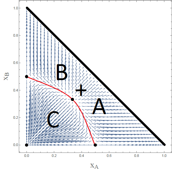
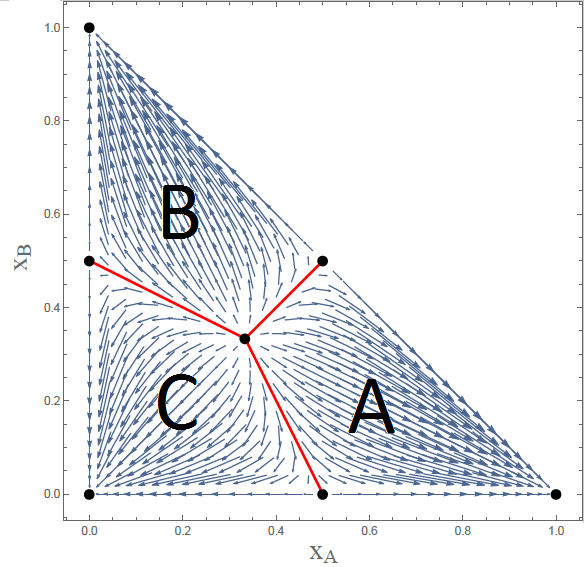
Understanding the behavior of the dynamics: From Figure B we see that when lies in the regime , we don’t understand the behavior of the system, e.g., we don’t know if we have explosion in the number of types (i.e., having types) in the long run. Moreover, we don’t know if the system reaches “stability” (in our notion).
- •
Relaxing the notion of stability: If we relax the notion of “stability” so that -fraction of the population is allowed to move ( does not move for some ), can we give better guarantees in Theorem 4.5?
References
- [1] A. Anagnostopoulos, R. Kumar, and M. Mahdian. Influence and correlation in social networks. 14th ACM SIGKDD International Conference on Knowledge Discovery and Data Mining, pages 7–15, 2008.
- [2] S. Aral, L. Muchnik, and A. Sundararajan. Distinguishing influence-based contagion from homophily-driven diffusion in dynamic networks. Proceedings of the National Academy of Sciences (PNAS), 2009.
- [3] S. Arora, Y. Rabani, and U. Vazirani. Simulating quadratic dynamical systems is pspace-complete (preliminary version). Proceedings of the Twenty-sixth Annual ACM Symposium on Theory of Computing (STOC), pages 459–467, 1994.
- [4] R. Axelrod. The dissemination of culture. Journal of Conflict Resolution, pages 203–226, 1997.
- [5] E. Bakshy, I. Rosenn, C. A. Marlow, and L. A. Adamic. The role of social networks in information diffusion. 21st International World Wide Web Conference, pages 203–226, 2012.
- [6] A. Bhattacharyya and K. Shiragur. How friends and non-determinism affect opinion dynamics. In 54th IEEE Conference on Decision and Control (CDC), pages 6466–6471, 2015.
- [7] J. M. Cohen. Sources of peer group homogeneity. Sociology in Education, pages 227–241, 1977.
- [8] G. Deffuant, D. Neau, F. Amblard, and G. Weisbuch. Mixing beliefs among interacting agents. Journal of Conflict Resolution, pages 87–98, 2000.
- [9] M. Feldman, N. Immorlica, B. Lucier, and S. M. Weinberg. Reaching consensus via non-bayesian asynchronous learning in social networks. In APPROX/RANDOM, pages 192–208, 2014.
- [10] S. Galam. Sociophysics: a review of Galam models. International Journal of Modern Physics C, 2008.
- [11] R. Hegselmann and U. Krause. Opinion dynamics and bounded confidence: models, analysis and simulation. Journal of Artificial Societies and Social Simulation, 2002.
- [12] R. A. Holley and T. M. Liggett. Ergodic theorems for weakly interacting infinite systems and the voter model. Annals of Probability, 1975.
- [13] M. O. Jackson. Social and economic networks. Princeton University Press, 2008.
- [14] D. B. Kandel. Homophily, selection, and socialization in adolescent friendships. American Journal of Sociology, pages 427–436, 1978.
- [15] J. L. Kelley. General Topology. Springer, 1955.
- [16] D. Kempe, J. M. Kleinberg, S. Oren, and A. Slivkins. Selection and influence in cultural dynamics. In ACM Conference on Electronic Commerce (EC), pages 585–586, 2013.
- [17] G. E. Kreindlera and H. P. Young. The spread of innovations in social networks. Proceedings of the National Academy of Sciences (PNAS), 2014.
- [18] T. LaFond and J. Neville. Randomization tests for distinguishing social influence and homophily effects. 19th International World Wide Web Conference, pages 601–610, 2010.
- [19] J. D. Lee, M. Simchowitz, M. I. Jordan, and B. Recht. Gradient descent only converges to minimizers. Conference on Learning Theory (COLT), 2016.
- [20] R. Mehta, I. Panageas, and G. Piliouras. Natural selection as an inhibitor of genetic diversity: Multiplicative weights updates algorithm and a conjecture of haploid genetics. Innovations in Theoretical Computer Science (ITCS), 2015.
- [21] R. Mehta, I. Panageas, G. Piliouras, P. Tetali, and V. V. Vazirani. Mutation, sexual reproduction and survival in dynamic environments. Innovations in Theoretical Computer Science (ITCS), 2017.
- [22] A. Montanari and A. Saberi. The spread of innovations in social networks. Proceedings of the National Academy of Sciences (PNAS), 2010.
- [23] E. Mossel, J. Neeman, and O. Tamuz. Majority dynamics and aggregation of information in social networks. In Autonomous Agents and Multi-Agent Systems (AAMAS), 2013.
- [24] I. Panageas and G. Piliouras. Average case performance of replicator dynamics in potential games via computing regions of attraction. ACM Conference on Economics and Computation (EC), 2016.
- [25] I. Panageas and G. Piliouras. Gradient descent only converges to minimizers: Non-isolated critical points and invariant regions. Innovations in Theoretical Computer Science (ITCS), 2017.
- [26] L. Perko. Differential Equations and Dynamical Systems. Springer, 3nd. edition, 1991.
- [27] K. Poole and H. Rosenthall. Patterns of congressional voting. American Journal of Political Science, pages 228–278, 1978.
- [28] Y. Rabinovich, A. Sinclair, and A. Widgerson. Quadratic dynamical systems. Proc 23rd IEEE Symp Foundations of Computer Science, pages 304–313, 1992.
- [29] M. Shub. Global Stability of Dynamical Systems. Springer-Verlag, 1987.
Appendix A Appendix
The following theorem holds for every separable metric space, i.e., every metric space that contains a countable, dense subset. In particular, we use this theorem for where is the number of types in the proof of Theorem 3.7.
Theorem A.1 (Lindelőf’s lemma [15]).
For every open cover there is a countable subcover.
The following lemma is used in Theorem 3.7 when we argue that the set of initial population vectors so that the dynamics converges to fixed points with an unstable direction, has measure zero. It roughly states that if a function is locally Lipschitz, then it preserves the measure zero sets (measure zero sets are mapped to measure zero sets).
Lemma A.2 (Null-set preserving, Appendix of [20]).
Let be a locally Lipschitz function with , then is null-set preserving, i.e., for if has measure zero then has also measure zero.
Proof.
Let be an open ball such that for all . We consider the union which cover by the assumption that is locally Lipschitz. By Lindelőf’s lemma we have a countable subcover, i.e., . Let . We will prove that has measure zero. Fix an . Since , we have that has measure zero, hence we can find a countable cover of open balls for , namely so that for all and also . Since we get that , namely cover and also for all . Assuming that ball (center and radius ) then it is clear that ( maps the center to and the radius to because of Lipschitz assumption). But , therefore and so we conclude that
Since was arbitrary, it follows that . To finish the proof, observe that therefore . ∎
Appendix B Figures