Distributed Event Localization via Alternating Direction Method of Multipliers
Abstract
This paper addresses the problem of distributed event localization using noisy range measurements with respect to sensors with known positions. Event localization is fundamental in many wireless sensor network applications such as homeland security, law enforcement, and environmental studies. However, most existing distributed algorithms require the target event to be within the convex hull of the deployed sensors. Based on the alternating direction method of multipliers (ADMM), we propose two scalable distributed algorithms named GS-ADMM and J-ADMM which do not require the target event to be within the convex hull of the deployed sensors. More specifically, the two algorithms can be implemented in a scenario in which the entire sensor network is divided into several clusters with cluster heads collecting measurements within each cluster and exchanging intermediate computation information to achieve localization consistency (consensus) across all clusters. This scenario is important in many applications such as homeland security and law enforcement. Simulation results confirm effectiveness of the proposed algorithms.
Index Terms:
Event localization, wireless sensor network, distributed algorithm.I Introduction
With the ability to transmit/receive information and fuse data, smart sensors enabled and greatly advanced numerous applications such as environmental monitoring [1], target tracking [2], underwater detection [3], and acoustic gunfire localization [4], [5]. Among these applications, event localization is a significant and essential component or even the ultimate goal. Taking the gunfire localization as an example, if some threat sources or impulsive events (e.g., shooting or explosion) occur, it is of imperative importance to localize these threat sources to make prompt reactions (e.g., giving warning, providing aid). In fact, sensor network based event localization has received significant attentions and plenty of techniques have been proposed in the literature, using either angle-of-arrival measurements [6, 7, 8], time-of-arrival (ToA) (including time-difference-of-arrival, i.e., TDoA) measurements [9, 10], or received signal strength (RSS) [11, 12, 13, 14, 15, 16, 17, 18]. There are also some work that discussed the event localization problem based on noisy range measurements directly, which can be obtained based on ToA, TDoA, or RSS information [19, 20, 21, 22, 23]. Generally speaking, these existing methods for event localization formulate the localization problem as a maximum likelihood estimation problem [21] or a least squares problem [17], which is solved by minimizing the non-convex objective function iteratively [11] or by applying various convex relaxations [10].
From the implementation point of view, existing event localization algorithms can be cast into two categories: centralized approaches and distributed approaches. Centralized approaches always gather (noisy) measurements (e.g., range measurements) obtained by all sensors to a processing center, which then estimates the event location using a certain centralized optimization algorithm. Typical centralized methods include the parallel projection method [20], convex relaxation plus semidefinite programming (SDP) or second-order cone programming method [10, 21, 15, 22, 16, 23, 17]. However, a severe shortcoming of centralized localization algorithms is that the computation complexity at the processing center might be quite high which poses great challenges for low-cost sensor nodes with limited computational capabilities. In addition, the required communication to collect all measurements to a single central node may be problematic due to possible traffic bottleneck and severe constraints on communication ranges. Moreover, once the central node fails due to, e.g., attacks or power depletion, the entire network slips into a state of paralysis. Therefore, techniques solving the event localization problem in a distributed way are crucial for sensor network based event localization.
In contrast to centralized algorithms, distributed localization algorithms are designed to run the computation over the entire network instead of on a processing center. In general, distributed algorithms are often established on massive parallelism or sequential calculations and mutual collaboration [24]. So compared with centralized algorithms, distributed designs have better scalability, flexibility, and failure resilience. One typical distributed approach for event localization is projection-based algorithms which solve the event localization problem by projecting an initial estimate onto sensing disks [11], circles [12, 13, 25], or rings [18]. However, these projection-based localization algorithms are very sensitive to the initial values when the target event lies outside the convex hull of sensors, as will be shown in Sec. 6.
This paper is motivated by acoustic event localization which is crucial on battlefields [26]. In such applications, the target event has no communication or computation capability, which differentiates the problem from sensor localization problems in which the locations of sensors are estimated [27]. Furthermore, in such applications, the target events lie outside the convex hull of deployed sensors, which renders existing projection-based algorithms inappropriate. SDP relaxation based algorithms can avoid the convex hull problem and are traditionally employed to solve the event localization problem [10, 21, 15, 22, 16, 23, 17]. However, as far as we known, existing SDP relaxation based algorithms for event localization are all centralized, with a central node collecting and processing all data, which makes them susceptible to processing center failure and traffic bottleneck. In this paper, we propose two distributed event localization approaches based on a clustered architecture motivated by mobile acoustic localization applications such as the PinPointTM system from BioMimetics Systems Inc. The PinPointTM mobile localization sensor network can be deployed as a mobile infrastructure for impulsive threat event detection and localization [26, 28]. Each PinPointTM sensor is a small omnidirectional microphone array which localizes impulsive acoustic events by correlating the ToA measurements among its microphone cells. In fact, since each sensor has an integrated microphone array, individual sensors are able to identify and localize a target event without assistance or cooperation with other sensors. However, due to close distances between the microphone cells, the accuracy of individual sensors is very limited and unsatisfactory, and collaboration among the sensors is necessary to improve localization accuracy [26, 28].
The above application motivated us to assume a localization architecture in which an entire network is divided into several clusters. A cluster head (which can be a regular sensor) collects and fuses measurements (e.g., noisy ranges) obtained from all members in its cluster. Two cluster heads in different clusters can exchange information (the local estimates of target events) if a communication link is available between them; otherwise they don’t have access to each other’s information. Our developed algorithms can also be applied in some other applications where a cluster-based architecture is employed. A typical example is the wide-area monitoring and control in large-scale power systems [29], [30]. To estimate the electro-mechanical oscillation modes, a large number of phasor measurement units (PMU) have to be deployed across a power network to conduct measurements. The measurements from PMUs have to be fused to diagnose the inter-area oscillation modes. However, wide-area communication between PMUs is very expensive [31]. To fuse information across the PMUs without imposing heavy communication overhead, a similar structure as ours is adopted in [29], [30]. Other examples on cluster-based architecture can be found in [32, 33, 34, 35].
The core of our distributed localization algorithms is the alternating direction method of multipliers (ADMM), which has been proven extremely suitable in distributed convex optimization, especially for large-scale problems [36]. The key idea of ADMM is to obtain a global solution through the cooperation of small local subproblems. ADMM is easy to parallelize and implement, and is robust to noise and computation errors [27]. Our proposed localization approaches take full advantages of ADMM which enables local optimizations within individual clusters as subproblems. Then through cooperation of subproblems in neighboring clusters, a global event localization could be reached. That is to say, the estimated locations obtained by individual clusters are made as consistent as possible. Such consistency is of crucial importance in many applications. For example, when a sporadic impulsive event requiring immediate responsive actions is detected by several monitors, consistency in the estimated location across monitors is the key for multiple monitors to coordinate cooperative operations.
Contribution: The main contribution of this paper is two ADMM-based distributed event localization algorithms, i.e., GS-ADMM and J-ADMM. Compared with existing centralized SDP relaxation based algorithms for event localization, the two algorithms divide the computation on a central node to different clusters to avoid possible center failure and traffic bottleneck, and in the mean time, guarantee consistency of the estimates across all clusters among which only limited communications are available. Furthermore, the two algorithms take advantages of SDP relaxation to avoid the convex hull problem compared with existing projection-based algorithms. Moreover, the algorithms are proven to converge with a convergence rate of where is the iteration time.
Organization: The rest of this paper is organized as follows: Section 2 states the formulation of the problem. To solve the problem, a convex relaxation is required and the method proposed by [27] is recapitulated in Section 3. In Section 4, two algorithms named GS-ADMM and J-ADMM are proposed based on ADMM, with their convergence properties analyzed in Section 5. Section 6 gives numerical simulation results. In the end, a conclusion is made in Section 7.
II PROBLEM STATEMENT
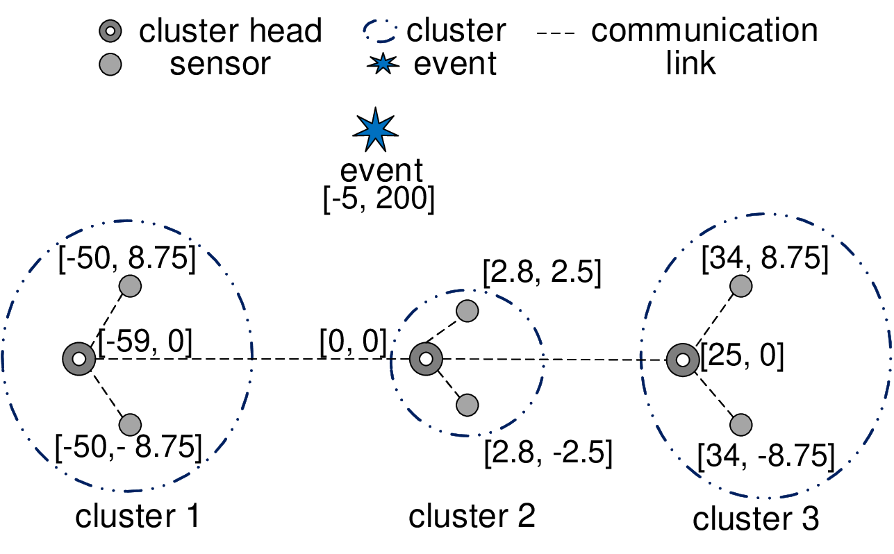
Motivated by mobile acoustic event localization applications such as the PinPointTM event localization sensor network [26, 28], we consider a localization sensor network divided into clusters (cf. Fig. 1 for the case ). Denote the number of constituent sensors of cluster as (). We consider localization in () dimensional Euclidean space and suppose that the position of the target event is denoted as . Denote the position of the th sensor in the th cluster as . The th sensor in the th cluster can obtain a noisy range measurement of its distance with respect to a target event:
where denotes the actual distance between the event position and the th sensor of the th cluster, and is the Gaussian noise term.

Then the event localization problem amounts to estimating the unknown event location using known sensor positions and noisy range measurements (). Still motivated by acoustic event localization applications (e.g., the PinPointTM event localization sensor network [26, 28]), we assume that a cluster head exists in each cluster , which can gather range measurements from all sensors within the cluster. In addition, a cluster head can communicate and exchange information with the cluster head of a neighboring cluster if there is a communication link between them (cf. Fig. 1). In this case, we also say that these two clusters can communicate. We assume that the communication pattern forms a connected network, i.e., there is a (multi-hop) path (composed of multiple communication links connected in succession) between any pair of cluster heads. For example, in Fig. 1, cluster 1 is able to exchange information with clusters 2 and 3 (via cluster heads); cluster 2 can exchange information with clusters 1, 3, and 4 (via cluster heads), etc. Denote as the set of all neighboring clusters of cluster , as the union of set and cluster itself, and as the number of clusters in .
As in most existing results, we use the maximum likelihood method for event localization [21, 22]. Let denote the measuring probability density function (PDF) for sensor in cluster and assume that it is a log-concave function of unknown distance [27], we can write this problem using the maximum likelihood method (which is costly but efficient [37]):
| (1) |
III CONVEX RELAXATION
Problem (1) is non-convex and it is generally infeasible to find a global optimal solution [27]. So a convex relaxation is needed to convert problem (1) into a convex optimization problem. Following the idea of [27], we use an SDP based relaxation approach. However, it is worth noting that there are inherent differences between the problem considered here and the sensor-position estimation problem in [27] where each sensor with unknown position estimates its own position using embedded computation capability. The differences are evident from the following example. Suppose that there is only one target to localize. In the case of [27], the target will be a sensor with unknown position and it estimates its own position alone using a centralized SDP based on all information gathered from adjacent sensors, including their positions and corresponding range measurements. Whereas in our case, the target is an event without any communication or computation capability and the event position estimation process is conducted cooperatively in a distributed way among the clusters.
To facilitate the relaxation, we first define the following new variables: , . Then we stack into and further stack into . In the same way we stack into and . Then the cost function can be written as
Consider the case of white zero-mean Gaussian noise, i.e., , then the above problem can be rewritten as
| (2) |
Without loss of generality, we can set the standard deviation in (2) to one. Now, problem (1) can be relaxed into the following constrained optimization problem:
| (3) | ||||
IV PROPOSED DISTRIBUTED ALGORITHMS
IV-A Preliminaries: Standard ADMM
ADMM is an algorithm which is suitable to solve problems in the following form [36]:
| (6) | ||||
where , , , , and , and and are convex functions. To get the optimal value for problem (6), one can first form an augmented Lagrangian function:
where is the Lagrange multiplier associated with the constraint and is a predefined penalty parameter. Then ADMM solves problem (6) by updating in the following sequence: first an -minimization step (7), then a -minimization step (8), and finally a dual variable update (9):
| (7) | |||
| (8) | |||
| (9) |
Next, we will propose two distributed algorithms for event localization using the framework of standard ADMM.
IV-B Problem Reformulation
In distributed algorithms, neighboring nodes have to generate and exchange copies of local estimates to ensure a consistent global estimation across all nodes. In our event localization architecture, a cluster is treated as a normal node which solves a common event localization problem based on measurements obtained by sensors within the cluster. And neighboring clusters exchange intermediate computational results (through cluster heads) to guarantee that all clusters reach the same estimation value.
To better interpret our algorithms, we define a local vector
which is owned by cluster .
We let denote the stacked vector of and define a convex set
IV-C ADMM based problem formulation
From the architecture in (11), it is easy to see that problem (10) can be divided into subproblems, which can be solved in a distributed way using ADMM by adding some constraints on . Next we present the basic idea based on a graph-based formulation of the communication pattern.
Using graph theory [39], the communication pattern of cluster heads can be represented by , where the set denotes the set of cluster heads, and denotes the set of undirected edges (communication links) between clusters. We use to denote the link (if there is) between cluster heads and . We use to represent the total number of undirected edges. In our problem formulation, each cluster is associated with a local cost function , and all clusters work together to solve the problem in (10). Assume that the local cost function is only known to cluster , then to reach consistency (consensus) of estimated position values among all clusters, we impose a constraint if there exists an edge between clusters and . Introduce a matrix , where denotes the dimensional identity matrix, then can be represented as . So the constraint can be represented as .
Now we are able to rewrite problem (10) into a distributed ADMM form as follows:
| (12) | ||||
or in a more compact way:
| (13) | ||||
where , , and is the edge-node incidence matrix of graph as defined in [40]. For example, in the one-dimensional case (), is an matrix whose rows correspond to the edges and columns correspond to the clusters such that:
| (14) |
Here we define that each edge originates at and terminates at .
It can be easily verified that the incidence matrix for Fig. 1 is
| (15) |
For high dimensional cases, where , can be obtained by replacing the value of and with and , respectively, with denoting the dimensional identity matrix. Then the matrix for Fig. 1 becomes
| (16) |
In this formulation, after each cluster obtains its local estimate , it sends the value (estimated event position ) to neighboring clusters. By adding the constraint as shown in (12), the consistency of individual event position () estimated across the clusters is guaranteed. Now we are in place to present our detailed algorithms to solve (12).
Remark 1
Note that although a normal way to apply ADMM to consensus problems is to create auxiliary local variables (cf. [27]), we just put the constraint directly here. The reason that we omit the auxiliary local variables is to save storage space at each cluster, since auxiliary local variables take additional storage space. Furthermore, by adding the constraint , we can have both a sequential and a parallel realization with convergence guaranteed, which will be detailed in the following subsection. This kind of constraint and its induced ADMM algorithm is called extended ADMM, which is discussed and applied in many recent work, e.g., [41, 29, 42, 40, 43].
IV-D Proposed Algorithms
Let be the Lagrange multiplier relevant to the constraint . Then the regularized augmented Lagrangian function of problem (12) can be reformulated as
| (17) | ||||
where are stacked into for all and are stacked into for all .
Applying ADMM, we can get the following two updating recursions:
| (18) | |||
| (19) |
Here, we can update in two different ways. One way is based on the Gauss-Seidel update [44] in which clusters update in a sequential order. The other way is the Jacobian scheme in which all clusters update in parallel [45].
Gauss-Seidel update (GS-ADMM): We first consider an algorithm based on the
Gauss-Seidel update. Gauss-Seidel update for distributed ADMM has
been explored theoretically and proven able to converge in most
cases for convex objective functions (see, e.g., [46, 47, 48]). GS-ADMM based solution for
distributed event localization can be described as follows:
Algorithm I: GS-ADMM
Each cluster initializes , .
Input: ,
Output: ,
- 1.
All clusters update their local vectors in a sequential order and send their local vectors to neighboring clusters in immediately, where
(20) Here we also consider the effect of when updating by adding a term . Problem (20) with given in (5) is an SDP problem that can be solved by common convex toolboxes such as Yalmip [27, 49], which is used in our simulations.
- 2.
Each cluster computes
(21) - 3.
Set , and go to 1).
In GS-ADMM, all clusters update their local estimated position values in a sequential way just as some projection-based algorithms. Sequential update can be used in small-size networks. For large-scale networks, a parallel method is more appropriate. So we also propose another algorithm based on Jacobian scheme which is amendable for parallelization.
Jacobian based ADMM (J-ADMM): Algorithm J-ADMM is motivated by the work in [42], which proposed the Proximal Jacobian ADMM by adding some proximal terms when updating .
We adopt the same idea here and prove that if the proximal terms meet some additional requirements, convergence of this algorithm can be guaranteed.
The detailed procedure of J-ADMM is given as follows, with the convergence analysis detailed in the following section.
Algorithm II: J-ADMM
Each cluster initializes , .
Input: ,
Output: ,
- 1.
Each cluster updates its local vector in parallel:
(22) - 2.
Each cluster sends its local vector to neighboring clusters in .
- 3.
Each cluster computes
(23) - 4.
Set , and go to 1).
Remark 2
A distinct difference between GS-ADMM and J-ADMM is the way they update . In GS-ADMM, each cluster updates its local estimated position value in a sequential way, which requires a globally predefined order. Whereas in J-ADMM, all clusters update their local estimated position values simultaneously. We remark that GS-ADMM is appropriate for small-scale sensor networks. But for large-scale networks, updating in a sequential way may be quite time-consuming and parallel methods like J-ADMM are more appropriate. So different updating methods should be chosen according to the size of networks and other practical concerns.
In fact, if we disregard the PinPointTM motivated application scenario, the proposed two algorithms can be completely distributed to each sensor by allowing sensors to have access to neighboring sensors’ positions and range measurements with respect to the target event. However, we argue that this, in fact, may cost more energy since each sensor has to solve an SDP problem. In addition, the required storage overhead is larger since each sensor has to store neighboring sensors’ positions and range measurements. Furthermore, consider a situation where two sensors can communicate with each other and have the same neighbors. Then the position estimation process conducted at these two sensors are the same, which leads to redundant processing of the same data. While in our clustered architecture, only cluster heads need to conduct position estimation and in fact, each sensor in the cluster can take turns to be the cluster head, which is helpful to average energy consumption. Compared with the iterative schemes, e.g., projection-based algorithms, where each sensor only has access to its own position and range measurement, our algorithms are insensitive to the convex hull problem. And compared with centralized SDP-based algorithms, our clustered architecture is robust to processing center failure or traffic bottleneck problems. In addition, the convex relaxation methods used at each cluster can be further improved by using recent works such as [10, 21, 15, 22, 16, 23, 17].
V CONVERGENCE ANALYSIS
In this section, we analyze the convergence properties of GS-ADMM and J-ADMM. As our algorithms are applications of distributed ADMM, the analysis benefits from many existing results on general distributed ADMM [40, 50, 41].
V-A Convergence Analysis of GS-ADMM
Let and be the iterates generated by algorithm GS-ADMM following (20) and (21). Assume that the initial problem (12) admits a solution , i.e., the Lagrangian function has a saddle point (note: not the augmented Lagrangian function), then the following theorem holds:
Theorem 1
Let be the average of up to iteration time , then the followings hold for all :
(1)
| (24) |
(2) The sequence deduced by GS-ADMM converge to , i.e., . In addition, we have .
Here
| (25) | ||||
and ().
Proof: (24) can be obtained following a way similar to Theorem 4.4 in [40]. A detailed proof is given in Appendix A. To prove the second statement, recall that the objective function is
Setting , we have . Note that is a quadratic function and is strongly convex. Since the sum of strongly convex functions is still strongly convex, our objective function is strongly convex. Further note that is equal to and the set is convex and closed. Therefore, our problem satisfies the requirements of both strongly convex objective function and convex-and-closed constraint set in [50]. Now we proceed to prove the second statement. First, rewriting in the form of , where denotes the columns of associated with cluster , we can form a variational inequality similar to (5)-(6) in [50]:
where
Then following the proof of Lemma 4.1 in [50], we can get that is a solution to if and hold. Secondly, following the proof of Lemma 4.2 in [50], we can get the following inequality:
where is strongly convex with modulus . Thirdly, define an auxiliary block-diagonal matrix :
Then by following the idea of the proof of Lemma 4.3 in [50], the following inequality can be obtained:
where
Finally, when holds, we can get the second statement following the proof of Theorem 4.1 in [50].
Remark 3
Recall , we can get
When , we have . In other words, . So can be represented as:
It is clear that will increase with an increase in , so if the iteration time is fixed, will also increase with an increase in . That is to say, with increasing, the iteration time to reach convergence will increase, namely convergence rate will be slower. Although with an increase in , the convergence rate will decrease, cannot be too small. This is because if is too small, the constraint is weak, which makes reaching consistency across clusters difficult. More detailed discussions on selecting can be found in [47].
Directly following the statements in Theorem 1, we can obtain the following result on the convergence speed:
Theorem 2
The convergence rate of GS-ADMM is , where is the iteration time.
Proof: The result can be obtained directly from the proof of Theorem 1 and is omitted.
V-B Convergence Analysis of J-ADMM
To analyze the convergence of J-ADMM, we first define several terms: Let and be the results for (22) and (23) for iteration . Augment the coefficients of proximal terms into a matrix and introduce a positive definite diagonal matrix , where is the number of clusters in . Since and are both diagonal matrices, we can define a new diagonal matrix according to where is the identity matrix. It can be easily verified that has the following form:
| (26) |
with for . Assuming that the original problem (12) admits a solution , then we have the following theorem:
Theorem 3
Let be the average of up to iteration time and denote the eigenvalues of as . If is true with , then the following holds for all :
| (27) |
where is the Lagrangian function, and
| (28) |
Proof: See Appendix B.
From Theorem 3, we can easily obtain the following results on the convergence speed:
Theorem 4
The convergence rate of J-ADMM is , where is the iteration time.
Proof: The result can be obtained directly from the proof of Theorem 3 and is omitted.
Since and are of the same form, Remark 3 for GS-ADMM also applies to the J-ADMM case. Next, we use numerical results to evaluate the performance of GS-ADMM and J-ADMM.
VI SIMULATION RESULTS
In this section, we illustrate effectiveness of the proposed approaches using comparison with existing results. A typical type of distributed algorithms for event localization is the projection-based algorithms. However, some projection-based algorithms, e.g., the DAPA algorithm in [18], is found in our simulations not appropriate for the considered case where the target event lies outside the convex hull of sensors. More specifically, we set the sensor localization architecture similar as in [51, 28], which considers a practical acoustic event localization system (see Fig. 2 for the detailed spatial distribution of all sensor nodes). The target event occurs at , which is far away from the nine sensors. Simulation results suggested that DAPA did not work well in this architecture, even if we set the initial values close to the target event and used the range measurements without noise, although it did work very well if the target event was set in the convex hull of sensors. In the simulation, we used the same parameters for DAPA as in [18], i.e., , , , and .
Then, we compared the localization performance of the proposed algorithms GS-ADMM and J-ADMM with two other projection-based algorithms: the PPM algorithm proposed in [20] and the PONLM algorithm proposed in [12], which gave reasonable performance in the simulations. PPM is a parallel projection method which requires a central node to average the local event location estimates obtained from all sensors in every iteration. PONLM is a sequential projection-based algorithm which solves the event localization problem by finding a point at the intersection of sensing circles. Both localization error (differences between estimated and actual target event positions) and localization consistency (differences in estimated positions between clusters) are compared under different noise standard deviations . The convergence performance is evaluated by exploring the evolution of the localization error with iteration time .
To facilitate comparison, we first define two performance indices:
Localization Error: we use the root mean square error (RMSE) to quantify the error between estimated and true positions for every cluster or sensor, which is denoted as :
where is the number of Monte Carlo trials, is the estimated position in the th Monte Carlo trial in a certain cluster or sensor, and is the true position of the target event.
Localization Inconsistency: We also use the root mean square error (RMSE) to quantify the localization inconsistency (difference) in estimated event positions between clusters, which is denoted as :
where is the number of Monte Carlo trials, is the estimated position obtained from the th cluster in the th Monte Carlo trial. is the number of clusters.
VI-A Convergence performance
We compared the convergence performance of our sequential GS-ADMM algorithm, parallel J-ADMM algorithm, the sequential PONLM algorithm in [12], and the parallel PPM algorithm in [20]. For GS-ADMM and J-ADMM, we set . For PPM and PONLM, we set the initial point at (PPM and PONLM are sensitive to initialization settings, which will be shown later). We used the range measurements without noise in this part. The simulation results are given in Fig. 3.
From Fig. 3, we can see that both GS-ADMM and J-ADMM reached an accuracy of after about 10 iterations, while PONLM took 25 iterations and PPM took about 150 iterations. Note that sensors and clusters have to exchange local estimates in each iteration, so the required communication overhead is heavier with an increase in iteration times. The same conclusion can be drawn for energy consumption. It is worth noting that both PPM and PONLM can reach very high accuracies. However, in practical applications like gunfire localization, the accuracy of is sufficient [28].

Remark 4
In our simulations, we used the Sedumi solver in Yalmip, whose limited precision may lead to approximate minima when solving subproblems (20) and (22). This may also lead to a low convergence speed or even fluctuations after a certain number of iterations. In addition, SeDuMi may sometimes return the message “Run into numerical problems”, which implies that it has terminated before it finds an approximate optimal solution [52]. In this situation, we can transform semi-definite inequality constraints into definite inequality constraints by introducing a constant positive definite term (e.g., ) as indicated in [53]. However, such a transformation may bring fluctuations to the convergence process.
VI-B The influence of noise level on
In this section, we simulated the event localization algorithms under different levels of Guassian noise standard deviation . For GS-ADMM and J-ADMM, we set . For PPM and PONLM, we ran simulations under two cases: setting fixed initial values at (denote as Fix in Table I) and setting random initial values in the area of 10000m 10000m (denote as Ran in Table I). The number of iterations is fixed to 50 for GS-ADMM, J-ADMM, PONLM, and 200 for PPM. All simulation results are summarized in Table I and Fig. 4. Each data point in Table I is an average of 100 Monte Carlo trials.
| GS-ADMM | J-ADMM | PPM | PONLM | |
|---|---|---|---|---|
| Fix Ran | Fix Ran | |||
| 0.00 | 0.3693 0.4848 0.5128 | 0.1146 0.2223 0.2964 | 0.2100 273.19 | 0.0338 304.52 |
| 0.01 | 0.5417 0.5443 0.5753 | 0.3546 0.3911 0.4385 | 0.2106 285.65 | 0.0498 269.86 |
| 0.02 | 0.5453 0.5862 0.5992 | 0.2766 0.3266 0.3779 | 0.2145 282.83 | 0.0865 307.95 |
| 0.05 | 0.6055 0.6723 0.7188 | 0.4987 0.5261 0.5724 | 0.2265 268.31 | 0.1895 278.84 |
| 0.10 | 1.0564 1.0942 1.1440 | 1.0562 1.0589 1.1017 | 0.2832 288.41 | 0.4019 243.67 |

From Table I, we can see that both PPM and PONLM reached high localization accuracies under fixed initial values. However, their performance deteriorated significantly when random initial values were used. Therefore PPM and PONLM are sensitive to initial value settings. If the target event lies outside the convex hull of sensors, the convergent values of PPM and PONLM may be far away from the true event position. GS-ADMM and J-ADMM can avoid the convex hull problem, so every estimate lay close to the true event position.
Fig. 4 visualizes the estimated event locations. Fig. 4 (a) and (b) show the localization results of the proposed algorithms GS-ADMM and J-ADMM respectively from 100 Monte Carlo trials with . Fig. 4 (c) and (d) show the results of PPM and PONLM respectively where the initial positions are chosen randomly. It is clear that both GS-ADMM and J-ADMM performed better than PPM and PONLM when the initial values are randomly chosen.
VI-C The influence of noise level on
Setting , we also evaluated the influence of noise level on of our proposed algorithms. The results are summarized in Fig. 5.

Fig. 5 indicates that the proposed GS-ADMM and J-ADMM have small localization inconsistency () under different noise strength. In other words, our proposed algorithms GS-ADMM and J-ADMM can achieve good consistency across clusters even under large noise standard deviations. As indicated before, consistency is of crucial importance in many applications.
VII CONCLUSIONS
We proposed two ADMM based distributed event localization algorithms GS-ADMM and J-ADMM that do not require the target event to be within the convex hull of the deployed sensors. Convergence properties of the algorithms are analyzed theoretically. Numerical simulations showed that the proposed algorithms are robust to measurement noises and insensitive to convex hull problem compared with existing projection-based algorithms.
Acknowledgments
We would like to thanks Dr. Andrea Simonetto for providing Matlab codes for his paper [27].
Appendix A Proof of (24) in Theorem 1
Lemma 1
Let and be the iterates generated by GS-ADMM following (20) and (21), then the following inequality holds for all :
| (29) | ||||
where is the edge-node incident matrix defined in (15), , and is the identity matrix. (In the following, we only consider belonging to the set , so we leave out this constraint in the following lemmas and proofs.)
Proof: Denote by the function
| (30) | ||||
From the update rule in (20), we know that is the optimizer of in the closed and convex set . Since and are convex, and is differentiable, following the proof of Lemma 3.1 in [54] (which is also mentioned in Lemma 1 in [55]), we can get
Substituting with (30), we have
Noting , using (21) leads to
Noting , from the definition of , we can rewrite the above inequality as
| (31) | ||||
here denotes the columns of associated with cluster .
Summing both sides of (31) over , and noticing that the following two equations hold [40],
we can get the lemma.
Lemma 2
Proof: Since for a scalar , holds, and recall , we can get
| (33) | ||||
In addition, as is the saddle point of the Lagrangian function , we have . So we can establish the following relationships using algebraic manipulation:
| (34) | ||||
| (35) | ||||
| (36) | ||||
| (37) | ||||
Adding and subtracting the term from the left side of (38), we can get
Now by applying (32) into the above inequality, the following inequality can be obtained:
Summing both sides of the inequality over , we can obtain the following result after some re-arrangement:
In addition, as our function is convex, we have , then we can get
Dividing both sides by yields
| (39) | ||||
Appendix B Proof of Theorem 3
To prove Theorem 3, we first introduce two lemmas:
Lemma 3
Proof: Denote by the function
| (41) | ||||
Then following the proof of Lemma 1, we can get
| (42) | ||||
Summing both sides of the above relation over , and noticing that the following two equations hold,
we can get the lemma.
Lemma 4
Proof: The proof is similar to the proof of Lemma 2 and is omitted.
Then following the proof of Theorem 1 (setting in (40) and applying (43)), we can obtain the following inequality:
Summing both sides of the above inequality over , we can get the following result after some re-arrangement:
Since , is a diagonal matrix with , we can get that the right hand side of the above inequality is greater than , which leads to
In addition, as our function is convex, we have and
By dividing both sides by , we can obtain
Combining the above relationship with the Lagrangian function , we can get Theorem 3.
References
- [1] P. Bonnet, J. Gehrke, and P. Seshadri. Querying the physical world. IEEE Personal Communications, 7(5):10–15, 2000.
- [2] V. Cevher, M. F. Duarte, and R. G. Baraniuk. Distributed target localization via spatial sparsity. In Proceedings of the 16th European Signal Processing Conference, pages 1–5, 2008.
- [3] J. Heidemann, Y. Li, A. Syed, J. Wills, and W. Ye. Underwater sensor networking: Research challenges and potential applications. Technical Report ISI-TR-2005-603, USC/Information Sciences Institute, 2005.
- [4] J. George and L. M. Kaplan. Shooter localization using a wireless sensor network of soldier-worn gunfire detection systems. Journal of Advances in Information Fusion, 8(1):15–32, 2013.
- [5] G. Simon, M. Maróti, Á. Lédeczi, G. Balogh, B. Kusy, A. Nádas, G. Pap, J. Sallai, and K. Frampton. Sensor network-based countersniper system. In Proceedings of the 2nd international conference on Embedded networked sensor systems, pages 1–12, 2004.
- [6] L. M. Kaplan, Q. Le, and P. Molnár. Maximum likelihood methods for bearings-only target localization. In Proceedings of the IEEE International Conference on Acoustics, Speech, and Signal Processing, volume 5, pages 3001–3004, 2001.
- [7] R. O. Schmidt. Multiple emitter location and signal parameter estimation. IEEE Transactions on Antennas and Propagation, 34(3):276–280, 1986.
- [8] M. Gavish and A. J. Weiss. Performance analysis of bearing-only target location algorithms. IEEE Transactions on Aerospace and Electronic Systems, 28(3):817–828, 1992.
- [9] K. C. Ho and W. Xu. An accurate algebraic solution for moving source location using TDOA and FDOA measurements. IEEE Transactions on Signal Processing, 52(9):2453–2463, 2004.
- [10] K. Yang, G. Wang, and Z. Q. Luo. Efficient convex relaxation methods for robust target localization by a sensor network using time differences of arrivals. IEEE Transactions on Signal Processing, 57(7):2775–2784, 2009.
- [11] D. Blatt and A. Hero. Energy-based sensor network source localization via projection onto convex sets. IEEE Transactions on Signal Processing, 54(9):3614–3619, 2006.
- [12] Q. Shi and C. He. Distributed source localization via projection onto the nearest local minimum. In 2008 IEEE International Conference on Acoustics, Speech and Signal Processing, pages 2553–2556, 2008.
- [13] J. Wang and P. Regalia. Sensor network localization via boundary projections. In CISS, pages 224–229, 2009.
- [14] W. Meng, W. Xiao, L. Xie, and A. Pandharipande. Diffusion based projection method for distributed source localization in wireless sensor networks. In 2011 IEEE Conference on Computer Communications Workshops, pages 537–542, 2011.
- [15] G. Wang. A semidefinite relaxation method for energy-based source localization in sensor networks. IEEE Transactions on Vehicular Technology, 60(5):2293–2301, 2011.
- [16] G. Wang, Y. Li, and R. Wang. New semidefinite relaxation method for acoustic energy-based source localization. IEEE Sensors Journal, 13(5):1514–1521, 2013.
- [17] J. Yuan, W. Ai, H. Deng, T. Shuai, and X. Zhao. Exact solution of an approximate weighted least squares estimate of energy-based source localization in sensor networks. IEEE Transactions on Vehicular Technology, 64(10):4645–4654, 2015.
- [18] Y. Zhang, Y. Lou, Y. Hong, and L. Xie. Distributed projection-based algorithms for source localization in wireless sensor networks. IEEE Transactions on Wireless Communications, 14(6):3131–3142, 2015.
- [19] A. Beck, P. Stoica, and J. Li. Exact and approximate solutions of source localization problems. IEEE Transactions on Signal Processing, 56(5):1770–1778, 2008.
- [20] T. Jia and R. M. Buehrer. A set-theoretic approach to collaborative position location for wireless networks. IEEE Transactions on Mobile Computing, 10(9):1264–1275, 2011.
- [21] O. Pinar, J. Gomes, J. Xavier, P. Oliveira, et al. A convex relaxation for approximate maximum-likelihood 2D source localization from range measurements. In 2010 IEEE International Conference on Acoustics, Speech and Signal Processing, pages 2698–2701, 2010.
- [22] X. Fu, F. Chan, W. K. Ma, and H. C. So. A complex-valued semidefinite relaxation approach for two-dimensional source localization using distance measurements and imperfect receiver positions. In 2012 IEEE 11th International Conference on Signal Processing, volume 2, pages 1491–1494, 2012.
- [23] P. Oğuz-Ekim, J. Gomes, J. Xavier, M. Stošić, and P. Oliveira. An angular approach for range-based approximate maximum likelihood source localization through convex relaxation. IEEE Transactions on Wireless Communications, 13(7):3951–3964, 2014.
- [24] J. Bachrach and C. Taylor. Localization in sensor networks. Handbook of sensor networks: Algorithms and Architectures, 1, 2005.
- [25] C. L. Wang, D. S. Wu, S. C. Chen, and K. J. Yang. A decentralized positioning scheme based on recursive weighted least squares optimization for wireless sensor networks. IEEE Transactions on Vehicular Technology, 64(10):4887–4893, 2015.
- [26] S. Deligeorges, G. Cakiades, J. George, Y. Q. Wang, and F. J. Doyle. A mobile self synchronizing smart sensor array for detection and localization of impulsive threat sources. In Proceedings of IEEE International Conference on Multisensor Fusion and Integration for Intelligent Systems, pages 351–356, 2015.
- [27] A. Simonetto and G. Leus. Distributed maximum likelihood sensor network localization. IEEE Transactions on Signal Processing, 62(6):1424–1437, 2014.
- [28] G. Cakiades, S. Desai, S. Deligeorges, B. E. Buckland, and J. George. Fusion solution for soldier wearable gunfire detection systems. In SPIE Defense, Security, and Sensing, pages 838802–838802, 2012.
- [29] S. Nabavi, J. H. Zhang, and A. Chakrabortty. Distributed optimization algorithms for wide-area oscillation monitoring in power systems using interregional PMU-PDC architectures. IEEE Transactions on Smart Grid, 6(5):2529–2538, 2015.
- [30] G. B. Giannakis, V. Kekatos, N. Gatsis, S. J. Kim, H. Zhu, and B. F. Wollenberg. Monitoring and optimization for power grids: A signal processing perspective. IEEE Signal Processing Magazine, 30(5):107–128, 2013.
- [31] R. Hasan, R. Bobba, and H. Khurana. Analyzing NASPInet data flows. In Proceedings of IEEE Power Systems Conference and Exposition, pages 1–6, 2009.
- [32] S. Venkatesan. Coordinating base stations for greater uplink spectral efficiency in a cellular network. In 2007 IEEE 18th International Symposium on Personal, Indoor and Mobile Radio Communications, pages 1–5, 2007.
- [33] A. Papadogiannis, D. Gesbert, and E. Hardouin. A dynamic clustering approach in wireless networks with multi-cell cooperative processing. In 2008 IEEE International Conference on Communications, pages 4033–4037, 2008.
- [34] J. Zhang, R. Chen, J. G. Andrews, A. Ghosh, and R. W. Heath. Networked MIMO with clustered linear precoding. IEEE Transactions on Wireless Communications, 8(4):1910–1921, 2009.
- [35] S. Jain, S. J. Kim, and G. B. Giannakis. Backhaul-constrained multicell cooperation leveraging sparsity and spectral clustering. IEEE Transactions on Wireless Communications, 15(2):899–912, 2016.
- [36] S. Boyd, N. Parikh, E. Chu, B. Peleato, and J. Eckstein. Distributed optimization and statistical learning via the alternating direction method of multipliers. Foundations and Trends in Machine Learning, 3(1):1–122, 2011.
- [37] A. Beck, M. Teboulle, and Z. Chikishev. Iterative minimization schemes for solving the single source localization problem. SIAM Journal on Optimization, 19(3):1397–1416, 2008.
- [38] D. V. Ouellette. Schur complements and statistics. Linear Algebra and its Applications, 36:187–295, 1981.
- [39] J. A. Bondy and U. S. R. Murty. Graph theory with applications, volume 290. Macmillan London, 1976.
- [40] E. Wei and A. Ozdaglar. Distributed alternating direction method of multipliers. In Proceedings of the 51st IEEE Conference on Decision and Control, pages 5445–5450, 2012.
- [41] J. Mota, J. Xavier, P. Aguiar, and M. Puschel. D-ADMM: A communication-efficient distributed algorithm for separable optimization. IEEE Transactions on Signal Processing, 61(10):2718–2723, 2013.
- [42] W. Deng, M. Lai, Z. Peng, and W. Yin. Parallel multi-block ADMM with O (1/k) convergence. Journal of Scientific Computing, 71(2):712–736, 2017.
- [43] K. Yuan, Q. Ling, and Z. Tian. Communication-efficient decentralized event monitoring in wireless sensor networks. IEEE Transactions on Parallel and Distributed Systems, 26(8):2198–2207, 2015.
- [44] G. H. Golub and C. F. Van Loan. Matrix computations, volume 3. Johns Hopkins University Press, 2012.
- [45] Y. Saad. Iterative methods for sparse linear systems. 2003.
- [46] B. S. He, M. Tao, and X. M. Yuan. Alternating direction method with gaussian back substitution for separable convex programming. SIAM Journal on Optimization, 22(2):313–340, 2012.
- [47] M. Hong and Z. Q. Luo. On the linear convergence of the alternating direction method of multipliers. Mathematical Programming, 162(1-2):165–199, 2017.
- [48] M. Tao and X. M. Yuan. Recovering low-rank and sparse components of matrices from incomplete and noisy observations. SIAM Journal on Optimization, 21(1):57–81, 2011.
- [49] J. Löfberg. Yalmip: A toolbox for modeling and optimization in MATLAB. In Proceedings of IEEE International Symposium on Computer Aided Control Systems Design, pages 284–289, 2004.
- [50] D. Han and X. Yuan. A note on the alternating direction method of multipliers. Journal of Optimization Theory and Applications, 155(1):227–238, 2012.
- [51] F. Núñez, Y. Q. Wang, D. Grasing, S. Desaic, G. Cakiadesc, and F. J. Doyle. Pulse-coupled time synchronization for distributed acoustic event detection using wireless sensor networks. Control Engineering Practice, 60:106–117, 2017.
- [52] H. Waki. How to generate weakly infeasible semidefinite programs via lasserre’s relaxations for polynomial optimization. Optimization Letters, pages 1–14.
- [53] D. Labit and K. Taitz. User’s guide for sedumi interface 1.04. 2002.
- [54] B. S. He and X. M. Yuan. On the o(1/n) convergence rate of the douglas–rachford alternating direction method. SIAM Journal on Numerical Analysis, 50(2):700–709, 2012.
- [55] J. Mota, J. Xavier, P. Aguiar, and M. Püschel. A proof of convergence for the alternating direction method of multipliers applied to polyhedral-constrained functions. arXiv preprint arXiv:1112.2295, 2011.