UV/Optical emission from the expanding envelopes of type II supernovae

We consider a spherically symmetric non-relativistic flow of an ideal fluid, with pressure dominated by radiation and approximating radiation transport by diffusion with constant opacity. Using Lagrangian coordinates, labeling a fluid element by the mass $m$ enclosed within the radius $r$ at which it is located, the radiation-hydrodynamics equations describing the evolution of the radius $r$, the velocity v, and the energy density $e$ of a fixed fluid element are

where $\rho=(4\pi r^{2})^{-1}\partial_{r}m$ is the density, $j$ is the energy flux (energy current density) and $p$ is the radiation pressure. The optical depth is given by $\tau(r)=\int_{r}^{\infty}\kappa\rho dr^{\prime}$. Gravity does not affect the flow of the ejecta significantly, and is therefore neglected. The equations were solved by a standard leap-frog method on a staggered-mesh, with a fully-implicit solver for the energy equation.

A stationary inner boundary condition, $\textrm{v}=0$ and $j=0$, and a free surface outer boundary condition, $\partial_{t}\textrm{v}=(\kappa/c)j$ and $e=0$, were imposed at $m=0$ and at $m=M$, respectively. The bolometric luminosity is not sensitive to the exact choice of the boundary condition at $m=M$, since it is determined by the diffusion through the optically thick layers [24, see]. Invoking an ad-hoc radiation flux-limiter is not required in our numeric calculations, since at $\tau\geq 1$ the flux is naturally limited at all times to $j/ce<0.5$ (at $\tau<1$ the flux is determined by the flux at $\tau\approx 1$, approximately satisfying $\nabla j=0$, and the energy density is unimportant). This also justifies our choice of the outer boundary conditions [8, see also].

In order to study the late time, $t>t_{\delta}$, behavior, we consider progenitors of radius $R$ and mass $M$, composed of a uniform density core of mass $M_{\rm c}$ and radius $R_{\rm c}\ll R$, surrounded by a polytropic envelope in hydrostatic equilibrium. At $t=0$ an energy $E$ is uniformly distributed within $r<R_{\rm c}/3$ to initiate the ”explosion”. In these calculations the entire mass $M$ is ejected, hence $M$ represents the ejecta mass (i.e. excluding the mass of a remnant). We consider $n=3/2$ and $n=3$ envelopes, a wide range of core to envelope masses, $0.1<M_{\rm c}/(M-M_{\rm c})<10$, a wide range of core to envelope radii, $10^{-3}<R_{\rm c}/R<10^{-1}$, and a wide range of radii, $10^{12}\mbox{ cm}<R<5\times 10^{13}\mbox{ cm}$. Figure 2 shows the initial density profiles for several $M_{\rm c}/(M-M_{\rm c})$ and $R_{\rm c}/R$ values, while figures 3 and 4 show the pressure and velocity profiles obtained at $t\approx R/\textrm{v}_{\rm s*}$. At late times, $t>5R/\textrm{v}_{\rm s*}$, the pressure and velocity profiles are not sensitive to the value of $R_{\rm c}/R$ for $R_{\rm c}/R<0.1$ (the fractional variations between the $R_{\rm c}/R=0.1,0.01$ and $R_{\rm c}/R=10^{-3}$ solutions are $\lesssim 10,1\%$; see also figs. 13 and 14). In what follows we present results for $R_{\rm c}/R=10^{-3}$, unless specifically stated otherwise.

We note, that the convergence of the initial density profiles to the $R_{\rm c}/R=10^{-3}$ profile is slower for $n=3$ compared to $n=3/2$ envelopes, see fig. 5. This, combined with the fact that the core radii of blue supergiants with radiative, $n=3$, envelopes may reach $R_{\rm c}/R\sim$ a few %, implies that the value of $f_{\rho}$ appropriate for such progenitors may depend on $R_{\rm c}/R$ and not only on $M_{\rm c}/M$. Although the dependence of the properties of the emission on $f_{\rho}$ is weak, the sensitivity of $f_{\rho}$ to $R_{\rm c}/R$ for large $R_{\rm c}/R$ and $n=3$ should be kept in mind (e.g. when inferring $E/M$ from $\textrm{v}_{*}$, see eq. 3 and § VI).

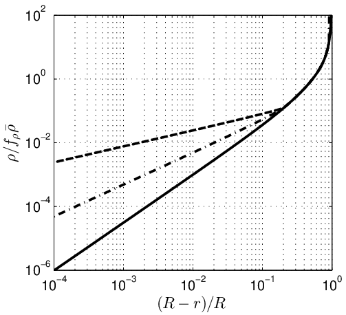
In order to study the dependence of the early time, $t<t_{\delta}$, behavior on deviations from polytropic profiles, we solve the radiation hydrodynamics equations for modified initial density profiles, where the density profile of an $n=3/2$ envelope is modified at the outer radii, $r>0.8R$, to $\rho_{0}\propto\delta^{\tilde{n}}$ with $\tilde{n}=0.5,1$ (keeping a continuous density at $r=0.8R$, see fig. 6). These modified profiles span the range of density profiles obtained by Morozova et al. [15] using the MESA and KEPLER stellar evolution codes at the relevant radii range (see their figure 2). We note, that the KEPLER profiles are not described at the outermost $\delta M/M<10^{-3}$ shells by a smooth power-law of the form given above. While this deviation may affect the breakout emission, it does not affect the post breakout emission discussed here, produced by deeper shells (see eq. 5 above and eq. 6 of RW11).

Figures 5 and 7 present the dependence on $M_{\rm c}/(M-M_{\rm c})=M_{\rm c}/M_{\rm env}$ of $f_{\rho}$ and of $\textrm{v}_{\rm s*}$ , normalized to the approximation suggested by Matzner & McKee [13], eq. (3). We find that the approximation of eq. (3) holds to better than 10% for $0.3<M_{\rm c}/M_{\rm env}<3$. The dependence of $f_{\rho}$ on $M_{\rm c}/M_{\rm env}$, approximately given by $f_{\rho}=(M_{\rm env}/M_{\rm c})^{1/2}$ and $f_{\rho}=0.08(M_{\rm env}/M_{\rm c})$ for $n=3/2$ and $n=3$, implies that, as expected, the relation between $\textrm{v}_{\rm s*}$ and $E/M$, which characterizes the bulk ejecta velocity, depends on the ejecta structure. In the absence of detailed information on the structure, $E/M$ may be inferred from $\textrm{v}_{\rm s*}$, which may be determined by early UV observations through eqs. (4), by $E/M=0.9[0.3]\textrm{v}_{\rm s*}^{2}$ for $n=3/2[3]$ with $5[30]\%$ accuracy for $0.3<M_{\rm c}/M_{\rm env}<3$. Conversely, a comparison of $\textrm{v}_{\rm s*}$, determined by early UV observations, and $E/M$, determined by other late time observations (e.g. spectroscopic ejecta velocity), will constrain the progenitor structure.

Figures 8 and 9 present the ratio of the final velocity, to which each fluid element is accelerated, to the velocity of the shock passing through this fluid element, $f_{\textrm{v}}(m)=\textrm{v}_{\rm f}/\textrm{v}_{\rm sh}$, for $n=3/2$ and $n=3$ respectively. We find that the spherical correction to the planar self-similar dynamics, described by $f_{\textrm{v}}$ and given by eq. 26 of Matzner & McKee [13], is accurate for the outer parts of the ejecta. In the inner parts, where the flow deviates from the self-similar solution, $f_{\textrm{v}}(m)$ also deviates from that given by Matzner & McKee [13] and depends on the detailed structure.

Figures 10-14 present the results of our numerical calculations for $T_{\rm eff}$ and $L$, where $T_{\rm eff}$ is defined through $L=4\pi r_{\rm ph}^{2}\sigma T_{\rm eff}^{4}$ and the photospheric radius is determined by $\tau(r_{\rm ph})=1$. The figures show the ratio between $T_{\rm eff}$ and $L$ obtained numerically and the analytic results of eqs. (4), with $f_{\rho}$ and $\textrm{v}_{\rm s*}$ determined from the numerical solutions, and with time normalized to

such that $t/t_{\rm tr}=\sqrt{8\pi\xi}$ (see eq. 6). $t_{\rm tr}$ is the time at which the envelope is expected to become transparent, i.e. satisfying $\tau\sim\kappa M_{\rm env}/4\pi\textrm{v}^{2}t^{2}=c/\textrm{v}$, noting that $\textrm{v}_{\rm f}\sim 2\textrm{v}$. Circles denote the time $t=R/5\textrm{v}_{\rm s*}$, after which the approximation of significant expansion is expected to hold. Results for polytropic envelopes are presented in solid lines, and for modified density profiles in dashed (dash-dotted) lines for $\tilde{n}=0.5(1)$. The figures clearly demonstrate that, as expected, the properties of the cooling envelope emission are not sensitive to the details of the density profile near the stellar surface. It should be noted here, that the photosphere lies within the layers of modified initial density at all times shown.

While Morozova et al. [15] show that the prescription of identifying the ”luminosity shell” with $\tau=c/\textrm{v}$ is inappropriate for shallow density profiles, our numerical results show that eqs. 4 with $n=3/2$ describe $L$ and $T$ also for $n<3/2$ envelopes. This can be explained by the weak $n$ dependence of both the luminosity and the temperature [5, note that the self-similar solutions are not physical for $n\lesssim 0.9$, where their luminosity diverges at $r\rightarrow 0$,].

At late time, $t>t_{\delta}$, radiation emerges from inner layers, the properties of which are not well approximated by the self-similar solution determined by eqs. (1) and  (2) (with post-breakout acceleration given by a fixed value of $f_{\textrm{v}}=\textrm{v}_{f}/\textrm{v}_{\rm s}$, see figs. 8 and 9). This leads to a suppression of the luminosity below the nearly time independent luminosity given by eq. (4), which is valid for $t<t_{\delta}$. The suppression of $L$ may be approximately described by the analytic expression (obtained by fitting to the numerical results)

with $A=0.94[0.79]$, $a=1.67[4.57]$ and $\alpha=0.8[0.73]$ for $n=3/2[3]$. This approximation holds to better than $20[30]\%$ up to $t=t_{\rm tr}/a$ for $n=3/2[3]$. The temperature is affected less strongly. For $n=3/2$, $T_{\rm eff}(t<0.5t_{\rm tr})$ is smaller than the self-similar result by $<10\%$ for $M_{\rm env}/M_{c}>>1$ and by $<20\%$ for $M_{\rm env}/M_{c}\leq 1$.

Figures 15 and 16 present the numerical results for the color temperature, $T_{\rm col}$, defined as the temperature of the plasma obtained in the numerical calculations (assuming local thermal equilibrium) at the ”thermalization depth” $r_{\rm ther}$, from which photons may diffuse to the photosphere without being absorbed. This radius is estimated as the radius for which the product of scattering and absorption optical depths equals unity, $\tau_{\rm sct}\tau_{\rm abs}\approx 1$ [14], approximately determined by (see RW11)

where $\kappa_{\rm abs}$ and $\kappa_{\rm sct}$ are the absorption and scattering opacities. The absorption opacity is determined as $k_{\rm abs}=k_{\rm R}-k_{\rm sct}$, with a Rosseland mean opacity, $k_{\rm R}$, given by the TOPS opacity tables [7] and $k_{\rm sct}$ evaluated using the number of free electrons provided by the tables¹¹ 1 Opacity and free electron number density tables were taken from http://aphysics2.lanl.gov/cgi-bin/opacrun/tops.pl.. This choice of the mean absorption opacity gives a higher weight to frequency bands where the total cross-section is small, through which radiation more readily escapes. In contrast with RW11, who used pure H:He mixtures, we consider here plasma compositions with solar and 0.1 solar metallicity [2]. We find that for $M_{\rm c}/M_{\rm env}\leq 1$, the ratio of $T_{\rm col}$, obtained from the numerical calculations, to $T_{\rm ph,RW}$, given by eq. (4), is $1.1[1.0]\pm 0.05$ for $n=3/2[3]$ in the relevant temperature range. For large values of $M_{\rm c}/M_{\rm env}$, $M_{\rm c}/M_{\rm env}=10$, $T_{\rm col}/T_{\rm ph,RW}$ is lower by $\approx 10\%$. The fact that $T_{\rm col}/T_{\rm ph}$ is close to unity suggests that the deviations from thermal spectra are not large, and that the spectral luminosity per unit wavelength $\lambda$ may be approximated by eq. (21), see § IV.3.

The decrease of $T_{\rm eff}$ below the self-similar result at $t\sim t_{\rm tr}$ is not reflected in the $T_{\rm col}$ plot of fig. 15, which shows the evolution only down to 0.7 eV. This is due to the fact that $T$ remains above 0.7 eV up to $t\sim t_{\rm tr}$ only for very low mass envelopes. For $n=3/2[3]$, $T_{\rm eff}(t=t_{\rm tr}/a)>0.7$ eV for

well below the envelope masses used for the numerical calculations shown in fig. 15. For low envelope masses and large stellar radii, the late time decrease of $T_{\rm eff}$, compared to the self-similar solution, is reflected in the color temperature at $T>0.7$ eV, as demonstrated in fig. 17.

We provide here a summary of the analytic formulae which, based on the comparison of the numerical results with eqs. 4, provide an approximate description of the post-breakout cooling emission at times (see eq. 5)

The bolometric luminosity is described at early time by the self-similar expression (see eq. 4)

with $\epsilon_{2}=0.086[0.175]$ for $n=3/2[3]$. The luminosity is suppressed at late time by a factor, which may be approximated by

with $A=0.94[0.79]$, $a=1.67[4.57]$ and $\alpha=0.8[0.73]$ for $n=3/2[3]$. This approximation holds for a wide range of $R_{\rm c}/R$ and $M_{\rm c}/M_{\rm env}$ values, $10^{-3}\leq R_{\rm c}/R\leq 10^{-1}$ and $0.1\leq M_{\rm c}/M_{\rm env}\leq 10$, to better than $20[30]\%$ from $t\sim 0.01t_{\rm tr}$ up to $t=t_{\rm tr}/a(n)$ for $n=3/2[3]$. $t=t_{\rm tr}$ is given by eq. (13),

The spectral luminosity per unit wavelength $\lambda$ may be approximated by (RW11)

where $g_{\rm BB}$ is the normalized Planck function,

and $T_{\rm col}$ is given by $T_{\rm col}/T_{\rm ph,RW}=1.1[1.0]\pm 0.05$ for $n=3/2[3]$ with weak sensitivity to metallicity in the relevant temperature range (for large radii, $R>10^{13.5}$ cm, and large values of $M_{\rm c}/M_{\rm env}$, $M_{\rm c}/M_{\rm env}=10$, $T_{\rm col}/T_{\rm ph}$ is lower by $\approx 10\%$; see figs. 15 and 16). $T_{\rm ph,RW}$ is given by eq. (4),

with $\epsilon_{1}=0.027[0.016]$ for $n=3/2[3]$.

The dependence of the results on $f_{\rho}$ is weak. For $R_{\rm c}/R\ll 1$, $f_{\rho}$ may be approximated by $f_{\rho}=(M_{\rm env}/M_{\rm c})^{1/2}$ and $f_{\rho}=0.08(M_{\rm env}/M_{\rm c})$ for $n=3/2$ and $n=3$ respectively (for progenitors with $n=3$ envelopes and large core radii, $R_{\rm c}/R\approx 0.1$, $f_{\rho}$ is larger by a factor of $\approx 3$ than the value given by this approximation, see fig. 5).

The above results are valid for $T>0.7$ eV, i.e. for

We have used numerical calculations to demonstrate that the early, $t<t_{\delta}=$few days (see eq. (5)), envelope cooling emission is not sensitive to the details of the density profile of the envelope (see figs. 10-14). The emission is well described by eqs. (4), with $T_{\rm ph}$ determined mainly by $R$, and $L$ determined mainly by $\textrm{v}_{\rm s*}^{2}R$. For $M_{\rm c}/M_{\rm env}\leq 1$, the ratio of $T_{\rm col}$ (see § IV.2, eqs. (21,22)), obtained from the numerical calculations, to $T_{\rm ph}$, given by eq. (4), is $1.1[1.0]\pm 0.05$ for $n=3/2[3]$, with weak sensitivity to metallicity in the relevant temperature range (this value is somewhat lower than that obtained in RW11, 1.2, who considered a pure He:H mixture; for large radii, $R>10^{13.5}$ cm, and large values of $M_{\rm c}/M_{\rm env}$, $M_{\rm c}/M_{\rm env}=10$, $T_{\rm col}/T_{\rm ph}$ is lower by $\approx 10\%$; see figs. 15 and  16).

The weak dependence of the early emission on the density structure, reflected in the very weak dependence of $T_{\rm col}/T_{\rm ph}$ and of $L$ and $T$ in eqs. (4) on $n$ and model parameters other than $R$ and $\textrm{v}_{\rm s*}^{2}$, implies that $R$ and $\textrm{v}_{\rm s*}^{2}$ may be inferred accurately and robustly from the observations of the early UV/optical emission.

The approximate relation between $\textrm{v}_{\rm s*}$ and $E/M$, given by eq. (3), holds to better than 10% for $0.3<M_{\rm c}/M_{\rm env}<3$ (see fig. 7). The dependence of $f_{\rho}$ on $n$ and on $M_{\rm c}/M_{\rm env}$, approximately given $R_{\rm c}/R\ll 1$ by $f_{\rho}=(M_{\rm env}/M_{\rm c})^{1/2}$ and $f_{\rho}=0.08(M_{\rm env}/M_{\rm c})$ for $n=3/2$ and $n=3$ (see fig. 5), implies that the relation between $\textrm{v}_{\rm s*}$ and $E/M$ depends on the ejecta structure. $E/M$ may be inferred from $\textrm{v}_{\rm s*}$ by $E/M=0.9[0.3]\textrm{v}_{\rm s*}^{2}$ for $n=3/2[3]$ with $5[30]\%$ accuracy for $0.3<M_{\rm c}/M_{\rm env}<3$ (for progenitors with $n=3$ envelopes and large core radii, $R_{\rm c}/R\approx 0.1$, $f_{\rho}$ is larger and $E/M=0.5\textrm{v}_{\rm s*}^{2}$ is a better approximation; see fig. 5). Conversely, a comparison of $\textrm{v}_{\rm s*}$, determined by early UV observations, and $E/M$, determined by other late time observations (e.g. spectroscopic ejecta velocity), will constrain the progenitor structure.

We have extended the solutions to $t\sim t_{\rm tr}$, see eq. (13), when the emission emerges from deep within the envelope and depends on the progenitor’s density profile. The expression given in the abstract for $t_{\rm tr}$ is obtained from eq. (13) using the approximation of eq. (3) for $\textrm{v}_{\rm s*}$, dropping for the sake of simplicity the dependence on $f_{\rho}$, $t_{\rm tr}=13f_{\rho}^{\beta/2}(M_{\rm env}/M_{\odot})^{3/4}(M/M_{\rm env})^{1/4}(E/10^{51}{\rm erg})^{-1/4}$ d.

We have shown (see § III) that the dependence of $L$ and $T$ on the progenitor parameters is of the general form of eq. (6), and used the numerical solutions to determine the dimensionless functions $f_{T}$ and $f_{L}$ for polytropic, $n=3/2$ and $n=3$, envelopes with a wide range of core to envelope mass and radius ratios, $0.1<M_{\rm c}/(M-M_{\rm c})<10$, $0.001<R_{\rm c}/R<0.1$. We have found that $T$ is well described by the analytic solution also at late time (for low mass envelopes $T$ may drop at late time by $\sim 20\%$ below the analytic prediction, see eq. 16 and fig. 17), while $L$ is suppressed by a factor which depends mainly on $n$ (and only weakly on $R_{\rm c}/R$ and $M_{\rm c}/M$), and may be approximated to $\approx 20\%$ accuracy up to $t=t_{\rm tr}/a(n)$ by the analytic approximations of eq. (14).

For very large progenitors, $R>10^{13.5}$ cm, with low mass envelopes, $M_{\rm env}\leq 1M_{\odot}$, the separation of the time scales $R/\textrm{v}_{\rm s*}$ and $t_{\rm tr}/a$ is not large, and the analytic expression for $L$ given by eqs. (4), which holds for $R/\textrm{v}_{\rm s*}\ll t\ll t_{\rm tr}/a$, is not accurate at any time. However, as demonstrated in fig. 13, the approximation for $L$ obtained using eqs. (4) with the suppression factor of eq. (14) is accurate to better than $10\%$ up to $t=0.1t_{\rm tr}$ also in this case. This implies that $R\textrm{v}_{\rm s*}^{2}$ (and hence $\textrm{v}_{\rm s*}^{2}$) may be accurately determined from the bolometric luminosity $L$ at early time also for very large progenitors, $R>10^{13.5}$ cm, with low mass envelopes.

It is worth noting, that the suppression of $L$ at $t>t_{\delta}$ implies that using eqs. (4) to infer $R$ from the luminosity observed at $t>t_{\delta}$ would lead to an under estimate of $R$ due to the overestimate of $L$, as demonstrated in fig. 18 (compare the solid and dashed curves) and as discussed by Rubin et al. [22].

We have shown (see fig. 18) that the suppression of $L$ at $t_{\rm tr}/a(n)$ obtained for standard polytropic envelopes may account for the first optical peak of double-peaked SN light curves, with first peak at a few days for $M_{\rm env}<1M_{\odot}$. The suppression of the bolometric luminosity is consistent with the observed behavior, and does not require a non-polytropic envelope with a special structure, e.g. where the the mass is initially concentrated at $r\sim R$. The time at which the bolometric luminosity is suppressed corresponds to $t_{\rm tr}/a(n)$ and hence constrains $M_{\rm env}/\textrm{v}_{\rm s*}$ (see eq. (13)), while the luminosity constrains $\textrm{v}_{\rm s*}^{2}R$. It is important to emphasize that these parameters cannot be determined accurately from the observations, since the emission at $t>t_{\delta}$ depends on the detailed structure of the progenitor (see discussion at the end of § V).

Finally, it is important to emphasize that our analysis holds as long as the opacity is approximately that of a fully ionized gas, i.e. for $T>0.7$ eV, $t<14R_{13.5}^{0.55}$ d. At lower temperatures, recombination leads to a strong decrease of the opacity (see fig. 1) and the photosphere penetrates deep into the ejecta, to a depth where the temperature is sufficiently high to maintain significant ionization and large opacity, implying that $T$ does not drop significantly below $\sim 0.7$ eV. This enhances the dependence on the details of the envelope structure and implies that detailed radiation transfer models are required to describe the emission (our simple approximations for the opacity no longer hold).

An accurate determination of $R$ requires an accurate determination of $T$ at a time when eq. (4) holds and $T$ depends mainly on $R$, i.e. when $T>0.7$ eV. An accurate determination of $T$ requires, in turn, observations at $\lambda<hc/4T=0.3(T/1{\rm eV})^{-1}\mu$, in order to identify the peak in the light curve, which is obtained when $T$ crosses $T_{\lambda}\approx hc/4\lambda$ (or by identifying the spectral peak provided redenning can be corrected for, RW11). Since the emission peaks below $0.3\mu$ for $T>1$ eV, UV observations at $\lambda<0.3~\mu$ (which must be carried out from space) will enable one to reliably determine $T$ and $R$ (and hence also $\textrm{v}_{\rm s*}$). On the other hand, observations at $\lambda\geq 0.44\mu$ (B-band or longer) corresponding to $T_{\lambda}=hc/4\lambda\leq 0.7$ eV, will not enable one to accurately determine $T$ and $R$. Observations in the U-band, $\lambda=0.36\mu$ corresponding to $hc/4\lambda=0.8$ eV, will provide less accurate results than UV observations due to the strong temperature dependence of the opacity at slightly lower temperature.

References

- [1] Arcavi, I. et al. 2011, ApJ, 742, L18, 1106.3551
- [2] Asplund, M., Grevesse, N., Sauval, A. J., & Scott, P. 2009, ARA&A, 47, 481, 0909.0948
- [3] Bersten, M. C. et al. 2012, ApJ, 757, 31, 1207.5975
- [4] Calzavara, A. J., & Matzner, C. D. 2004, MNRAS, 351, 694, astro-ph/0312464
- [5] Chevalier, R. A. 1992, ApJ, 394, 599
- [6] Chevalier, R. A., & Fransson, C. 2008, ApJ, 683, L135, 0806.0371
- [7] Colgan, J. et al. 2016, ApJ, 817, 116, 1601.01005
- [8] Ensman, L., & Burrows, A. 1992, ApJ, 393, 742
- [9] Gandel’Man, G. M., & Frank-Kamenetskii, D. A. 1956, Soviet Physics Doklady, 1, 223
- [10] Ganot, N. et al. 2016, ApJ, 820, 57, 1412.4063
- [11] Kasen, D., Metzger, B. D., & Bildsten, L. 2015, ArXiv e-prints, 1507.03645
- [12] Katz, B., Sapir, N., & Waxman, E. 2012, ApJ, 747, 147, 1103.5276
- [13] Matzner, C. D., & McKee, C. F. 1999, ApJ, 510, 379, astro-ph/9807046
- [14] Mihalas, D., & Mihalas, B. W. 1984, Foundations of radiation hydrodynamics (New York, Oxford University Press)
- [15] Morozova, V., Piro, A. L., Renzo, M., & Ott, C. D. 2016, ArXiv e-prints, 1603.08530
- [16] Nakar, E., & Piro, A. L. 2014, ApJ, 788, 193, 1401.7013
- [17] Nakar, E., & Sari, R. 2010, ApJ, 725, 904, 1004.2496
- [18] Nicholl, M., & Smartt, S. J. 2015, ArXiv e-prints, 1511.03740
- [19] Nicholl, M. et al. 2015, ApJ, 807, L18, 1505.01078
- [20] Piro, A. L. 2015, ApJ, 808, L51, 1505.07103
- [21] Rabinak, I., & Waxman, E. 2011, ApJ, 728, 63, 1002.3414
- [22] Rubin, A. et al. 2015, ArXiv e-prints, 1512.00733
- [23] Sakurai, A. 1960, Commun. Pure Appl. Math., 13, 353, 13, 353
- [24] Sapir, N., Katz, B., & Waxman, E. 2011, ApJ, 742, 36, 1103.5075
- [25] ——. 2013, ApJ, 774, 79, 1304.6428
- [26] Van Dyk, S. D. et al. 2014, AJ, 147, 37, 1312.3984
- [27] Waxman, E., & Katz, B. 2016, ArXiv e-prints, 1607.01293
- [28] Waxman, E., Mészáros, P., & Campana, S. 2007, ApJ, 667, 351, astro-ph/0702450
- [29] Wheeler, J. C. et al. 1993, ApJ, 417, L71
- [30] Woosley, S. E., Eastman, R. G., Weaver, T. A., & Pinto, P. A. 1994, ApJ, 429, 300