Universal crossover from ground state to excited-state quantum criticality

We begin by introducing a simple one-dimensional model, the so-called Fibonacci chain (also called the golden chain), whose eigenstates exhibit quantum critical properties, with different critical exponents and universal classes in the ground state and in highly excited states. This “spin” chain is constructed in analogy with the spin-$\frac{1}{2}$ Heisenberg model $H=\sum_{i}J_{i}\vec{S}_{i}\cdot\vec{S}_{i+1}$ for which the nearest neighbor interaction gives a different energy to the singlet and triplet channels in the tensor product (fusion) $\frac{1}{2}\otimes\frac{1}{2}=0\oplus 1$, where we labeled the irreducible representations of $SU(2)$ by their spin $j=0,\frac{1}{2},1,\dots$. Whereas the $SU(2)$ group has infinitely many irreducible representations, it is useful to think of models similar to the spin-$\frac{1}{2}$ Heisenberg chain where the number of “spins” is truncated. The Fibonacci chain is an example of such truncation of the Heisenberg chain, and models a chain of non-Abelian anyons carrying a nontrivial topological charge $\tau$, with the fusion property

In analogy with the Heisenberg chain, the Hamiltonian of such a system would then take the form

where $J_{i}$ are the interaction strength which are drawn from some random distribution and $P_{i}^{A}$ is the singlet projection operator (projection to the trivial anyon) between site $i$ and $i+1$. Contrary to the fusion rule for $SU(2)$ spins $\frac{1}{2}$, Eq. 1 implies that the Hilbert space of $N+1$ anyons is equal to the $N$th Fibonacci number $F_{N}$, where $F_{1}=1=F_{2}$, and $F_{n+1}=F_{n}+F_{n-1}$ which scales asymptotically as $\varphi^{N}$ where $\varphi=\frac{1+\sqrt{5}}{2}$ is the golden ratio. This implies that each Fibonacci anyon has quantum dimension, $\varphi$, an irrational number. This implies that the Hilbert space of the Fibonacci chain cannot be described as a tensor product of local degrees of freedom. The precise definition of the Hilbert space and of the expression of the Hamiltonian (2) is reviewed in Appendix A, in relation with the more general $SU(2)_{k}$ anyonic chains (the Fibonacci case corresponding to $k=3$). Beyond the potential relevance of this one-dimensional Hamiltonian in the context of topological quantum computation [36] (where it could be realized as a quasi-one-dimensional trench of anyonic excitations of a topologically ordered phase), we find it useful to think of anyonic chains such as (2) as a convenient lattice regularization of critical points that would be multi-critical (and therefore highly fine-tuned) in regular spin chains. For example, at zero temperature anyonic chains with uniform couplings are known to provide a very natural lattice regularization of the minimal models of conformal field theory [41], and their ground states in the presence of strong disorder correspond [39] to the so-called Damle-Huse infinite randomness fixed points [42].

Similar to ordinary disordered spin chains [43, 23, 24, 25], the ground state ($T=0$) properties of the disordered Fibonacci chain (2) can be obtained [37, 38, 39] via strong-disorder, real-space renormalization group (RSRG) methods. The key idea of this approach is to focus on the strongest bond of the chain $\Omega=\left|J_{i}\right|$, which at strong disorder will be typically much larger than its neighbors $\Omega\gg\left|J_{i+1}\right|,\left|J_{i-1}\right|$. We can then diagonalize this strong bond by choosing the singlet channel for an antiferromagnetic (AF) strong coupling $J_{i}>0$, or the triplet channel for a ferromagnetic (FM) strong coupling $J_{i}<0$. In the singlet channel, the two Fibonacci anyons on sites $i$ and $i+1$ form a singlet and quantum fluctuations induce an effective second-order coupling $J_{\rm eff}=\frac{2}{\varphi^{2}}\frac{J_{L}J_{R}}{J_{i}^{2}}$ between the anyons on sites $i-1$ and $i+2$. In the triplet channel, the Fibonacci anyons on sites $i$ and $i+1$ instead form an effective new Fibonacci anyon that interacts with its neighbors via the first order couplings $-\frac{J_{L/R}}{\varphi}$. These decimation rules conserve the form of the original Hamiltonian and are summarized in Fig. 1. While this RSRG is a priori approximate and accurate only at strong disorder, the effective disorder strength increases along the RG flow so that this method becomes “asymptotically exact” and yields exact predictions for universal properties such as critical exponents.

This RSRG approach predicts that the ground state of the random Fibonacci chain is in a random-singlet phase, an infinite randomness quantum critical point characterized by algebraically decaying averaged correlation functions [24, 25, 44], logarithmic scaling of entanglement [45], and energy-length scaling [25, 44]

instead of the usual quantum-critical relation $E\sim L^{-z}$. The exponent $\psi$ in Eq. (3) is given by $\psi=\frac{\Pi_{s}}{1+\Pi_{s}}$, where $\Pi_{s}$ is the probability that an RG step results in a second-order decimation by fusing two anyons into a singlet. For an antiferromagnetic chain [37], all decimated bonds are fused to a singlet $\Pi_{s}=1$, so that $\psi_{\rm AF}=\frac{1}{2}$. Introducing a finite fraction of ferromagnetic bonds can be argued to be a relevant perturbation to this AF fixed point [38], and the system flows to a fixed point [42] with equal ratio of F and AF bonds, so that $\Pi_{s}=\frac{1}{2}$ and $\psi_{\rm F/AF}=\frac{1}{3}$.

The ground-state RSRG described above can be straightforwardly generalized to target many-body excited states by observing that at each step, it is possible to project the strong bond onto an excited-state manifold [16]. The resulting excited-state RSRG (RSRG-X) iteratively resolves smaller and smaller energy gaps, corresponding to slow modes in the dynamics [26, 27], and allows one to construct, in principle, all the many-body eigenstates of the system [16, 22] (see also 29, 28, 32). For our example of the Fibonacci chain Eq. (2), one identifies and diagonalizes the strongest bond $\Omega$ in the chain just like the ground-state version. However, instead of automatically choosing the fusion channel with minimal energy, one can choose to sometimes increase the total energy by choosing higher energy fusion channels. The whole many-body spectrum can in principle be obtained in this way, and every eigenstate corresponds to a “branch” in the tree of choices between singlet and triplet channels at each step of the RG (Fig. 2). For instance, the ground state (the zero-temperature sampling [43, 23, 24, 25, 38]) can be obtained by following the branch with the lowest energy, i.e., by choosing the singlet (triplet) channel if the strong bond is antiferromagnetic (ferromagnetic).

Even if RSRG-X allows one to construct in principle all the many-body eigenstates, computing physical quantities remains a very complicated task due to the exponential size of the Hilbert space. However, $T=\infty$ properties can be simply obtained by noting that for entropic reasons, typical eigenstates in the middle of the many-body spectrum can be targeted by performing a random walk on the tree of many-body eigenstates [22]. This amounts to choosing a fusion channel (or a branch) with a probability based on the dimension of the Hilbert space of the effective chain after decimation. In the Fibonacci chain with $N+1$ anyons, this means we should weight the singlet channel with probability $F_{N-2}/F_{N}$ and the triplet branch with probability $F_{N-1}/F_{N}$ to ensure that each branch (or each eigenstate) is given the same probability by the RG ($T=\infty$). When $N$ is large, these probabilities converge to $1/\varphi^{2}$ and $1/\varphi$, respectively. From now on, for notational convenience we will fix $\Pi_{s}=1/\varphi^{2}$ to be the singlet fusion probability at infinite temperature. The critical behavior of $T=\infty$ eigenstates is therefore given by a RG flow similar to $T=0$, but where the probability to fuse to a singlet at each RG step is governed by entropy maximization rather than energy minimization. The $T=\infty$ RSRG-X still flows to an infinite-randomness fixed point characterized by the scaling (3), but with a new infinite-temperature tunneling exponent:

different from the $T=0$ exponents $\psi_{\rm AF}=\frac{1}{2}$ and $\psi_{\rm F/AF}=\frac{1}{3}$. Dimerization is irrelevant at the infinite-temperature fixed point [22] (this is related to the impossibility of many-body localizing Fibonacci anyons [47]), and the resulting $T=\infty$ critical phase was dubbed quantum critical glass (QCG) in Ref. 22, and is characterized by a non-ergodic logarithmic scaling of eigenstate entanglement $S\sim\ln L$ violating ETH, and by algebraic decaying averaged correlation functions. Although there is no formal proof for the stability of this non-ergodic critical phase against thermalization as in the MBL case [48], several arguments [26, 14] suggest it is stable at strong enough disorder, while for weak disorder, the proliferation of many-body resonances ignored by RSRG-X naturally leads to thermalization [49]. Regardless of this question of stability of QCG in the thermodynamic limit, we remark that RSRG-X can be made arbitrarily accurate for any finite size system by increasing the disorder strength.

We emphasize that this QCG nonergodic phase is very different from “marginal MBL” critical points that arise in the random transverse field Ising chain for example, for which the ground-state critical behavior simply extends to finite energy density. In the random Fibonacci chain, the ground state and excited states of the system belong to completely different universality classes, characterized by distinct RG fixed points. Moreover, random Fibonacci anyons are generically critical and cannot be many-body localized [47]—even by strongly dimerizing the couplings [22]—so that the QCG state should be considered as a (nonequilibrium) phase, rather than a fine-tuned critical point.

As we will see in detail in the following, finite temperature or energy density is a relevant perturbation to the $T=0$ fixed points, so that the system flows to the $T=\infty$ QCG fixed point for all temperatures $T>0$. The corresponding schematic RG flows are sketched in Fig. 3 and the goal of this paper is to study the (universal) finite-temperature crossover between the $T=0$ and $T=\infty$ behaviors. We now turn to how finite-temperature properties can be efficiently obtained using RSRG-X.

As we argued in the introduction, a physically motivated way to interpolate between the $T=0$ and $T=\infty$ quantum critical behaviors is to weight finite energy density eigenstates by a Boltzmann distribution. We emphasize however that we are dealing with an isolated non-ergodic system, so that the effective temperature $T$ is used merely as a way to target the properties of finite energy density eigenstates. The expectation is that typical eigenstates with similar energy density, $\epsilon$, have the same bond distribution, and since the Boltzmann distribution produces uncertainty in energy density that scales like $\Delta\epsilon\sim 1/\sqrt{L}$ where $L$ is the system size, that this sampling method enables us to reproduce the dynamical scaling properties of a more generic quench from an arbitrary non-eigenstate with typical energy density $\epsilon$. Within RSRG-X, this means that we want to sample eigenstates with energy $E$ according to a Boltzmann distribution ${\rm e}^{-\beta E}/Z$.

In Ref. 16, it was demonstrated that this could be done numerically using a Monte Carlo sampling using the Metropolis algorithm [50]. This Monte Carlo sampling of the RSRG-X tree of eigenstates can be summarized as follows: let us start with a single eigenstate (corresponding to a given branch in the tree), which we call a sample eigenstate, with energy $E_{s}$. We make a trial move by picking a random eigenstate, a trial eigenstate, with energy $E_{t}$. We accept the move if $e^{-\beta E_{t}}/e^{-\beta E_{s}}$ is larger than a random number in an interval $[0,1]$. If the trial state is accepted, then the trial state becomes a sample eigenstate and if not, then the sample eigenstate remains the same. At the end of each attempt, we compute some desired quantities, e.g., the entanglement entropy or some correlation function, and because of the detailed balance condition we are guaranteed to sample eigenstates according to the Boltzmann distribution at $\beta$. Even though this Monte Carlo sampling is a powerful tool that allows one to partly overcome the exponential number of eigenstates, generating a random eigenstate requires some computation time and limits the system size to ${\it O}(100)$ sites. This number might be too small to capture the fixed point coupling distribution which would require at least $10^{4}$ spins. Another disadvantage of the Monte Carlo sampling is that it gets harder upon approaching zero temperature because, since each trial eigenstate is chosen randomly, it is exponentially hard to sample exactly the ground state at zero temperature as the system size becomes larger.

Because of these complications, we seek an analytically tractable alternative to Monte Carlo sampling. To this end, we note that a sampling method that leads to analytically tractable flow equations is to independently weight the fusion choice locally at each node of the RSRG-X tree (Fig. 2), rather than globally based on the entire energy of the branch. Namely, consider the following local-node weighting scheme. If the strongest bond is antiferromagnetic, $J_{i}>0$, then we choose the singlet branch with probability $p_{A}^{1}=\frac{\Pi_{s}e^{\beta\Omega}}{(1-\Pi_{s})+\Pi_{s}e^{\beta\Omega}}$ and choose the triplet branch with probability $p_{A}^{\tau}=\frac{1-\Pi_{s}}{(1-\Pi_{s})+\Pi_{s}e^{\beta\Omega}}$. Otherwise, if the strongest bond is ferromagnetic, $J_{i}<0$, then we choose the singlet branch with probability $p_{F}^{1}=\frac{\Pi_{s}e^{-\beta\Omega}}{(1-\Pi_{s})+\Pi_{s}e^{-\beta\Omega}}$ and choose the triplet branch with probability $p_{F}^{\tau}=\frac{1-\Pi_{s}}{(1-\Pi_{s})+\Pi_{s}e^{-\beta\Omega}}$. By sending $\beta$ either to infinity or zero, this “local-node sampling” reduces to the zero or infinite temperature cases, and at first glance, one might hope that it correctly interpolates between these limits giving the desired Boltzmann sampling of many-body eigenstates. However, this local-node sampling turns out to actually deviate from the desired Boltzmann distribution on eigenstates, as we will argue shortly for a simple four-site system. Nonetheless, we will demonstrate that local-node sampling actually provides a very good approximation at strong disorder, and hence will ultimately be successful for computing universal scaling properties due to the flow to strong disorder.

To see that the local-node weighting scheme deviates from the desired global-branch Boltzmann weighting for finite temperatures $0<T<\infty$, let us consider a simplified 4-state model where 4 eigenstates correspond to 4 branches at the end of the RG-tree. This model is different from the Fibonacci anyon chain and would arise for instance for an Ising chain, but it captures the essence of the local node sampling in the most simplified fashion. Our model system is described in Fig. 4. The energies are given by $E_{1,1}+E_{2,1}$, $E_{1,1}+E_{2,2}$, $E_{1,2}+E_{2,3}$, and $E_{1,2}+E_{2,4}$ with the associated Boltzmann probabilities $\frac{1}{Z}e^{-\beta(E_{1,1}+E_{2,1})}$, $\frac{1}{Z}e^{-\beta(E_{1,1}+E_{2,2})}$, $\frac{1}{Z}e^{-\beta(E_{1,2}+E_{2,3})}$, and $\frac{1}{Z}e^{-\beta(E_{1,2}+E_{2,4})}$, where $Z=e^{-\beta(E_{1,1}+E_{2,1})}+e^{-\beta(E_{1,1}+E_{2,2})}+e^{-\beta(E_{1,2}+E_{2,3})}+e^{-\beta(E_{1,2}+E_{2,4})}=e^{-\beta E_{1,1}}(e^{-\beta E_{2,1}}+e^{-\beta E_{2,2}})+e^{-\beta E_{1,2}}(e^{-\beta E_{2,3}}+e^{-\beta E_{2,4}})$ is the partition function. The probability of choosing the ground state in the local node sampling is given by the product of choosing a lower branch in RG step 1, $p_{1}$, and the probability of choosing a lower branch in RG step 2, $p_{2}$. Note that the dimension of the Hilbert space of a lower and an upper branch are the same at each RG step; we get $p_{1}=\frac{e^{-\beta E_{1,1}}}{e^{-\beta E_{1,1}}+e^{-\beta E_{1,2}}}$ and $p_{2}=\frac{e^{-\beta E_{2,1}}}{e^{-\beta E_{2,1}}+e^{-\beta E_{2,2}}}$. Hence the local node probability associated with the ground state is $p_{1}p_{2}=\frac{1}{Z^{\prime}}e^{-\beta(E_{1,1}+E_{2,1})}$, where $Z^{\prime}=e^{-\beta E_{1,1}}(e^{-\beta E_{2,1}}+e^{-\beta E_{2,2}})+e^{-\beta E_{1,2}}(e^{-\beta E_{2,1}}+e^{-\beta E_{2,2}})$ which is different from $Z$. All the other eigenstates suffer from the same problem, resulting from the fact that $E_{2,1},E_{2,2}\neq E_{2,3},E_{2,4}$, meaning that the energies involved in the second decimation are influenced by the outcome of the first decimation.

Despite this discrepancy, this local node sampling approximation can be justified analytically by analyzing the history dependence of the RG flow, that is, by quantifying how much a choice of fusion channel at energy scale $\Gamma_{0}$ affects the rest of the RG flow for $\Gamma>\Gamma_{0}$. As we have seen above, the difference between the local node and the true Boltzmann samplings comes from this history dependence: if the choice of fusion channel in the first step affects the energy at a later step (in our example, $E_{2,1},E_{2,2}\neq E_{2,3},E_{2,4}$), then the two samplings will be different. In practice though, a given decimation will not affect most of the subsequent RG steps that will most likely involve bonds far away from it, but it will modify the energy when the renormalized bonds resulting from the original decimation are decimated again.

When one decimates a strong bond with strength $\Omega_{0}=e^{-\Gamma_{0}}$, there are two options: either a singlet is formed with some probability leading to a strongly weakened renormalized coupling $\sim J_{L}J_{R}/\Omega_{0}$ between the neighboring anyons, or a new effective anyon $\tau$ is created with two effective couplings to its neighbors given by first-order perturbation theory. If we choose the singlet channel, the renormalized second-order coupling is typically much weaker than most bonds in the chain, so that it will be decimated much later in the flow. Generalizing the ideas of Ref. 45, we find that it will typically be decimated at scale $\Gamma_{s}=\Gamma_{0}e^{\Pi_{s}(2+\Pi_{s})}$ where for simplicity, we assumed that the singlet fusion probability $\Pi_{s}$ is constant over this range of energy scales. This will lead to a contribution of order $\Omega_{s}\sim\Omega_{0}^{e^{\Pi_{s}(2+\Pi_{s})}}$ to the energy. If on the other hand we pick the $\tau$ channel at scale $\Gamma_{0}$, we find that the resulting first order couplings will typically be decimated at scale $\Gamma_{\rm\tau}=\Gamma_{0}e^{\Pi_{s}(1+\Pi_{s})}$ leading to a term in the many-body energy of order $\Omega_{\tau}\sim\Omega_{0}^{e^{\Pi_{s}(1+\Pi_{s})}}$. The crucial point is that these decimations will occur much later in the RG, and give contributions to the energy $\Omega_{1}$ or $\Omega_{\tau}$ that are negligible compared to $\Omega_{0}$ in the strong-disorder limit $\Omega_{0}\to 0$ ($\Gamma_{0}\to\infty$). This implies that in the strong-disorder limit, a given decimation will essentially not affect the subsequent flow so that the local-node sampling will become an increasingly good approximation of the Boltzmann distribution.

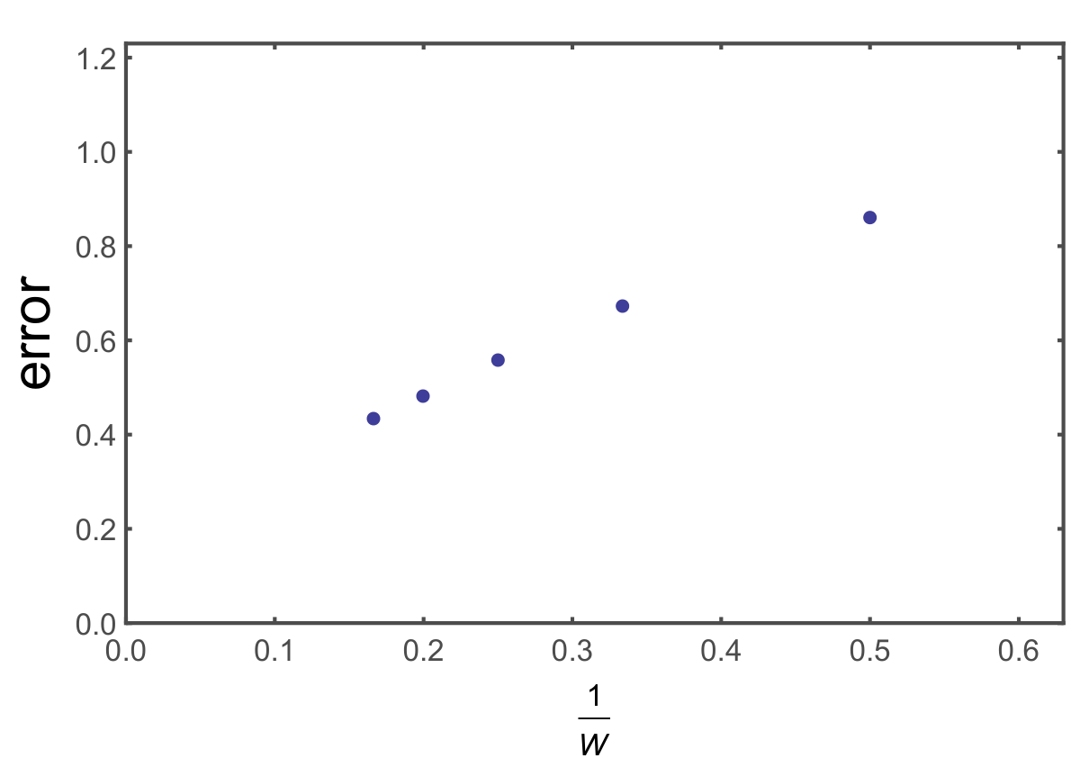
In agreement with this analytical argument, we will show numerically in the following that the local-node sampling using $(p_{A}^{1},p_{A}^{\tau},p_{F}^{1},p_{F}^{\tau})$ is a good approximation of the Boltzmann sampling with an error that decreases upon increasing the initial disorder strength. This implies that the local-node sampling using $(p_{A}^{1},p_{A}^{\tau},p_{F}^{1},p_{F}^{\tau})$ captures the correct universal long-time dynamics at finite $\beta$ since the disorder strength increases without bound along the RG flow.

To see how the local-node sampling works in practice, we plot the probability given to eigenstates using the local node sampling as a function of energy for $10^{3}$ eigenstates drawn randomly in a disordered Fibonacci chain with $10^{3}$ anyons (Fig. 5). The initial couplings are drawn from $P(\log J^{-1})=\frac{1}{W}e^{-\frac{\log J^{-1}}{W}}$, where $W$ is the initial disorder strength. We used RSRG-X at infinite temperature to sample eigenstates randomly and set $W=2$. The probability is then computed by a local node probability $(p_{A}^{1},p_{A}^{\tau},p_{F}^{1},p_{F}^{\tau})$ with $\beta=1$ and $0$. We find that the local node sampling gives a distribution very close to the Boltzmann result, with an effective fitted temperature $\beta\approx 0.99$ which agrees with the correct value. We remark that the data at infinite temperature ($\beta=0$) shows a small splitting instead of a perfect horizontal line because we used the expression $\Pi_{s}=1/\varphi^{2}$ to weight the different fusion channels, which is exact in the thermodynamic limit but which differs from the exact expression $F_{N-2}/F_{N}$ when the number $N$ of remaining anyons becomes small near the end of the renormalization process.

To quantify the difference between Boltzmann and local-node sampling, recall that the local-node sampling associates the probability $p_{i}=e^{-\beta E_{i}}/Z_{\textrm{eff}}^{(i)}$ with an eigenstate $i$, where $E_{i}$ is the energy and $Z_{\textrm{eff}}^{(i)}$ is the guessed (effective) partition function of $i$. Ideally, the effective partition function should be independent of the eigenstate, and should coincide with the actual partition function at temperature $\beta^{-1}$. To see how the accuracy of the local-node sampling changes upon increasing the initial disorder strength, we compute the averaged standard deviations of the guessed (or effective) partition function as the error as we vary the initial disorder strength $W$. We averaged over $500$ disorder realizations with $10^{3}$ spins and we sample $10^{3}$ eigenstates randomly to calculate the standard deviation of the effective partition function. It is clear from Fig. 6 that the error decreases as we increase the disorder strength, which implies that the local-node sampling becomes a better approximation upon increasing the disorder strength. Since the disorder strength increases without bound along the RG flow, we expect that the local-node sampling captures the correct long-time, universal behavior of the system. We note that the nonzero value of the extrapolated error at $W=\infty$ is a finite-size artifact, and appears to vanish in the infinite-system limit.

We note in passing that it might be possible to interpolate between the exact – but numerically costly – Boltzmann (Monte Carlo) sampling and our asymptotically exact – approximate but analytically tractable – local-node sampling. To be more specific, one could imagine choosing trial states of the Monte Carlo procedure by following the local-node sampling at desired temperature $\beta^{-1}$, while accepting or rejecting the trial states by using both the probability given by the exact Boltzmann factor and the probability associated with the local-node sampling. This kind of “assisted” Monte Carlo sampling method has appeared in the literature recently [51, 52] and was been shown to be much more efficient than conventional Monte Carlo samplings. It will be interesting to investigate such improved Monte Carlo samplings in the future.

As we have seen in the previous section, the simple local-node Boltzmann weighting of the RG fusion branches $(p_{A}^{1},p_{A}^{\tau},p_{F}^{1},p_{F}^{\tau})$ gives arbitrary good approximation to the Boltzmann distribution at strong disorder, and can therefore be expected to accurately capture the universal finite-temperature crossover physics. Using this local node probability, we can derive analytic finite-temperature RG flow equations for the disordered Fibonacci chain in a way that is very similar to the $T=0$ and $T=\infty$ cases. These flow equations encode how the coupling distribution evolves along the RG flow. It is convenient to define the energy scale at a given RG step by $\Omega=\max_{i}|J_{i}|$, the RG scale $\Gamma=\log(\frac{1}{\Omega})$, and logarithmic couplings $\zeta_{i}=\log\frac{\Omega}{|J_{i}|}$. (We normalize the initial energy scale to be $\Omega_{0}=1$.) The full flow equations are derived in Appendix B, and they read

where $\rho_{A}$ and $\rho_{F}$ are the probability distribution of the coupling strength of antiferromagnetic and ferromagnetic bonds, $p_{A}^{1}=p_{A}^{1}(\beta;\Gamma)=\frac{\Pi_{s}e^{\beta\Omega}}{(1-\Pi_{s})+\Pi_{s}e^{\beta\Omega}}$ and $p_{F}^{1}=p_{F}^{1}(\beta;\Gamma)=\frac{\Pi_{s}e^{-\beta\Omega}}{(1-\Pi_{s})+\Pi_{s}e^{-\beta\Omega}}$ are singlet fusion probabilities of an antiferromagentic/ferromagnetic bond at an energy-scale $\Omega=e^{-\Gamma}$, and $\rho_{1}\star\rho_{2}=\int_{0}^{\zeta}d\zeta^{\prime}\rho_{1}(\zeta-\zeta^{\prime},\Gamma)\rho_{2}(\zeta^{\prime},\Gamma)$ is the convolution between the two distributions $\rho_{1}$ and $\rho_{2}$. $\rho_{A}$ and $\rho_{F}$ are normalized in such a way that $p_{A}=\int d\zeta\rho_{A}(\zeta,\Gamma)$ and $p_{F}=\int d\zeta\rho_{F}(\zeta,\Gamma)$ are the ratio of the total antiferromagnetic and ferromagnetic bonds at the RG scale $\Gamma$. Equation (5) reduce to the zero or the infinite temperature flow equations [38, 22] by sending $\beta$ to infinity or zero. One powerful feature of these flow equations is that they describe the flow of couplings associated with a single typical eigenstate under the RG flow at the desired energy density (or temperature). This again shows a great advantage over the Monte Carlo sampling which requires reasonably many samplings in order to obtain finite-temperature properties.

Like the flow equations at zero and infinite temperature, Eqs. (5) admit a remarkably simple fixed-point (or scale-invariant) solution. Using a stability analysis, one can show that the fixed-point distribution has equal proportion of ferromagnetic and antiferromagnetic bonds, so that $\rho_{A}(\zeta,\Gamma)=\rho_{F}(\zeta,\Gamma)$. Let us therefore define $\rho(\zeta,\Gamma)=2\rho_{A}(\zeta,\Gamma)=2\rho_{F}(\zeta,\Gamma)$, so that the flow equations (5) reduce to

where $\Pi_{s}(\beta)=\Pi_{s}(\beta;\Gamma)=\frac{1}{2}(p_{A}^{1}+p_{F}^{1})$ is the averaged singlet fusion probability. The fixed-point solution thus reads $\rho(\zeta,\Gamma)=\frac{1}{W+\Xi_{s}(\beta;\Gamma)}e^{-\frac{\zeta}{W+\Xi_{s}(\beta;\Gamma)}}$, where $\Xi_{s}=\int_{0}^{\Gamma}d\Gamma^{\prime}\Pi_{s}(\beta;\Gamma^{\prime})$ is the integral of $\Pi_{s}(\beta;\Gamma)$. Note that the Ising ($k=2)$ case has constant $\Pi_{s}(\beta)=1$, i.e., the flow equation is the same as the ground state and at infinite temperature and there is no crossover (so that there is no difference between the ground state and excited states in this case; see also 31, 46).

The averaged singlet fusion probability $\Pi_{s}(\beta;\Gamma)$ determines how fast the effective disorder strength changes as we increase the RG parameter $\Gamma$. Upon increasing $\Gamma$, $\Pi_{s}(\beta;\Gamma)$ exhibits a crossover from the zero-temperature value $\Pi^{0}_{s}=\frac{1}{2}$ to the infinite-temperature value $\Pi^{\infty}_{s}=\Pi_{s}=\frac{1}{1+\tau}$ around the energy scale $\Omega\sim 1/\beta$. We expect physical quantities such as correlation functions or entanglement entropy to show a crossover interpolating between the $T=0$ and $T=\infty$ critical properties as a function of, say, distance $L$. In order to determine how the scaling between energy and distance evolves along the crossover, we need to determine how the scaling between energy and length evolves along the flow. This can be computed by noting that as we increase the RG scale from $\Gamma$ to $\Gamma+d\Gamma$, the number of decimated spins is given by $dN=-N(\Gamma)\rho(0,\Gamma)\big(1+\Pi_{s}(\beta;\Gamma)\big)d\Gamma$. Using the fixed-point solution, the typical distance between spins at scale $\Gamma$ is equal to:

where $N_{0}$ is the initial number of spins and $N(\Gamma)$ is the number of spins at scale $\Gamma$. (Note also that we set our initial energy scale to unit, $\Omega_{0}=1$.) At high energy or short distances, $\Pi_{s}(\beta;\Gamma)$ is close to its UV (ultraviolet) value and we have the random-singlet scaling $\Gamma\sim L^{\psi_{0}}$ with $\psi_{0}=\frac{\Pi^{0}_{s}}{1+\Pi^{0}_{s}}=\frac{1}{3}$, while in the IR (low energy), the scaling between energy and length is modified to $\Gamma\sim L^{\psi_{\infty}}$ with a different, smaller exponent $\psi_{\infty}=\frac{\Pi^{\infty}_{s}}{1+\Pi^{\infty}_{s}}$. As the crossover takes place when $\Omega\sim 1/\beta$, two length scales $L_{0}=L_{0}(\beta)$ and $L_{\infty}=L_{\infty}(\beta)$ naturally emerge below and above which the physics is captured by the zero and infinite temperature infinite-randomness fixed points, respectively. This finite-temperature crossover is summarized in Fig. 7 which shows that at any temperature $T>0$, the system eventually flows to the infinite-temperature fixed point responsible for the large-scale and long-time behavior, after crossing over from the zero-temperature random-singlet phase.

To illustrate how physical quantities scale along the crossover, let us consider for example the typical behavior of the two-point correlation function obtained by measuring the projection operator onto the singlet channel of two sites separated by distance $L$, which we denote by suggestive short-hand notation $\langle\vec{S}_{0}\cdot\vec{S}_{L}\rangle_{T}$ (with this shorthand notation, the Hamiltonian of our Fibonacci chain can be written as $H=\sum J_{i}\vec{S}_{i}\cdot\vec{S}_{i+1}$ as for an ordinary Heisenberg spin chain). At zero and infinite temperature, the typical behavior of this correlation function is governed by a stretched exponential decay $\sim{\rm e}^{-\alpha L^{\psi_{0,\infty}}}$ (averaged correlation functions should instead decay algebraically because of rare events that dominate the average). At finite temperature, it is given by the typical virtual coupling between sites at distance $L$,

where $\overline{\xi}=W+\Xi_{s}(\beta;\Gamma)$ and $\Gamma(L)$ is obtained by inverting Eq. (7). Taking the scaling limit $T\to 0$ and $L\to\infty$ of Eq. (8) numerically while keeping $L/L_{0}(\beta)$ fixed [recall that $L_{0}(\beta)\sim(\log\beta)^{1/\psi_{0}}$], we find that the typical spin-spin correlation function obeys the following universal scaling

where $C$ is a non-universal (cutoff dependent) constant, $\psi_{0}=\frac{1}{3}$, and $f(x)$ is a universal scaling function that interpolates between $f(0)=1$ in the UV and $\lim_{x\rightarrow\infty}f(x)\sim x^{\psi_{\infty}-\psi_{0}}$ in the IR (Fig. 8).

The full functional form of the crossover function $f(x)$ can be computed in closed form by approximating the double-exponential Boltzmann factors of the form $e^{-\beta\Omega_{0}e^{-\Gamma}}$ in $\Pi_{s}(\beta;\Gamma)$ by step functions, from which we find

This function is plotted in dashed lines in Fig. 8, and produces close agreement with the numerical evaluation of Eq. (7) using the exact form of $\Pi_{s}(\beta;\Gamma)$.

This computation demonstrates the methodology for computing universal crossover scaling of other quantities, including mean correlation functions as well as more complicated observables such as entanglement entropy [45, 38].

References

- [1] S. Sachdev, Quantum Phase Transitions, 2nd ed. (Cambridge University Press, Cambridge, 2011).
- [2] P. W. Anderson, Phys. Rev. 109, 1492 (1958).
- [3] L. Fleishman and P. Anderson, Phys. Rev. B 21, 2366 (1980).
- [4] I. Gornyi, A. Mirlin, and D. Polyakov, Phys. Rev. Lett. 95, 206603 (2005).
- [5] D. Basko, I. Aleiner, and B. Altshuler, Annals of Physics 321, 1126 (2006).
- [6] V. Oganesyan and D. A. Huse, Phys. Rev. B 75, 155111 (2007).
- [7] A. Pal and D. A. Huse, Phys. Rev. B 82, 174411 (2010).
- [8] R. Nandkishore and D. A. Huse, Annual Review of Condensed Matter Physics 6, 15 (2015).
- [9] B. Bauer and C. Nayak, Journal of Statistical Mechanics: Theory and Experiment 2013, P09005 (2013).
- [10] M. Serbyn, Z. Papić, and D. A. Abanin, Phys. Rev. Lett. 111, 127201 (2013).
- [11] S. Gopalakrishnan and R. Nandkishore, Phys. Rev. B 90, 224203 (2014).
- [12] D. J. Luitz, N. Laflorencie, and F. Alet, Phys. Rev. B 91, 081103 (2015).
- [13] R. Vosk, D. A. Huse, and E. Altman, Phys. Rev. X 5, 031032 (2015).
- [14] A. C. Potter, R. Vasseur, and S. A. Parameswaran, Phys. Rev. X 5, 031033 (2015).
- [15] D. A. Huse, R. Nandkishore, V. Oganesyan, A. Pal, and S. L. Sondhi, Phys. Rev. B 88, 014206 (2013).
- [16] D. Pekker, G. Refael, E. Altman, E. Demler, and V. Oganesyan, Phys. Rev. X 4, 11052 (2014).
- [17] A. Chandran, V. Khemani, C. R. Laumann, and S. L. Sondhi, Phys. Rev. B 89, 144201 (2014).
- [18] Y. Bahri, R. Vosk, E. Altman, and A. Vishwanath, Nat Commun 6 (2015).
- [19] J. A. Kjäll, J. H. Bardarson, and F. Pollmann, Phys. Rev. Lett. 113, 107204 (2014).
- [20] K. Slagle, Z. Bi, Y.-Z. You, and C. Xu, ArXiv e-prints (2015), arXiv:1505.05147 [cond-mat.str-el] .
- [21] A. C. Potter and A. Vishwanath, ArXiv e-prints (2015), arXiv:1506.00592 [cond-mat.dis-nn] .
- [22] R. Vasseur, A. C. Potter, and S. A. Parameswaran, Phys. Rev. Lett. 114, 217201 (2015).
- [23] S.-k. Ma, C. Dasgupta, and C.-k. Hu, Phys. Rev. Lett. 43, 1434 (1979).
- [24] D. S. Fisher, Phys. Rev. Lett. 69, 534 (1992).
- [25] D. S. Fisher, Phys. Rev. B 50, 3799 (1994).
- [26] R. Vosk and E. Altman, Phys. Rev. Lett. 110, 067204 (2013).
- [27] R. Vosk and E. Altman, Phys. Rev. Lett. 112, 217204 (2014).
- [28] Y.-Z. You, X.-L. Qi, and C. Xu, Phys. Rev. B 93, 104205 (2016).
- [29] C. Monthus, Journal of Statistical Mechanics: Theory and Experiment 2016, 033101 (2016).
- [30] K. Agarwal, E. Demler, and I. Martin, Phys. Rev. B 92, 184203 (2015).
- [31] Y. Huang and J. E. Moore, Phys. Rev. B 90, 220202 (2014).
- [32] R. Vasseur, A. J. Friedman, S. A. Parameswaran, and A. C. Potter, Phys. Rev. B 93, 134207 (2016).
- [33] K. Slagle, Y.-Z. You, and C. Xu, Phys. Rev. B 94, 014205 (2016).
- [34] D. A. Huse, R. Nandkishore, and V. Oganesyan, Phys. Rev. B 90, 174202 (2014).
- [35] A. Feiguin, S. Trebst, A. W. W. Ludwig, M. Troyer, A. Kitaev, Z. Wang, and M. H. Freedman, Phys. Rev. Lett. 98, 160409 (2007).
- [36] C. Nayak, S. H. Simon, A. Stern, M. Freedman, and S. Das Sarma, Rev. Mod. Phys. 80, 1083 (2008).
- [37] N. E. Bonesteel and K. Yang, Phys. Rev. Lett. 99, 140405 (2007).
- [38] L. Fidkowski, G. Refael, N. E. Bonesteel, and J. E. Moore, Phys. Rev. B 78, 224204 (2008).
- [39] L. Fidkowski, H.-H. Lin, P. Titum, and G. Refael, Phys. Rev. B 79, 155120 (2009).
- [40] R. Nandkishore, S. Gopalakrishnan, and D. A. Huse, Phys. Rev. B 90, 064203 (2014).
- [41] S. Trebst, M. Troyer, Z. Wang, and A. W. W. Ludwig, Progress of Theoretical Physics Supplement 176, 384 (2008).
- [42] K. Damle and D. A. Huse, Phys. Rev. Lett. 89, 277203 (2002).
- [43] C. Dasgupta and S.-k. Ma, Phys. Rev. B 22, 1305 (1980).
- [44] D. S. Fisher, Phys. Rev. B 51, 6411 (1995).
- [45] G. Refael and J. E. Moore, Phys. Rev. Lett. 93, 260602 (2004).
- [46] M. Pouranvari and K. Yang, Phys. Rev. B 92, 245134 (2015).
- [47] A. C. Potter and R. Vasseur, Phys. Rev. B 94, 224206 (2016).
- [48] J. Z. Imbrie, Phys. Rev. Lett. 117, 027201 (2016).
- [49] A. Chandran, M. D. Schulz, and F. J. Burnell, Phys. Rev. B 94, 235122 (2016).
- [50] N. Metropolis, A. W. Rosenbluth, M. N. Rosenbluth, A. H. Teller, and E. Teller, The journal of chemical physics 21, 1087 (1953).
- [51] L. Huang and L. Wang, Phys. Rev. B 95, 035105 (2017).
- [52] J. Liu, Y. Qi, Z. Y. Meng, and L. Fu, Phys. Rev. B 95, 041101 (2017).
- [53] Z. Wang, Topological quantum computation, 112 (American Mathematical Soc., 2010).