Gravitationally induced particle production and its impact on structure formation
Abstract
In this paper we investigate the influence of a continuous particles creation processes on the linear and nonlinear matter clustering, and its consequences on the weak lensing effect induced by structure formation. We study the line of sight behavior of the contribution to the bispectrum signal at a given angular multipole , showing that the scale where the nonlinear growth overcomes the linear effect depends strongly of particles creation rate.
Keywords:
structure formation; dark matter; cosmological matter creationpacs
98.80.-k; 95.35.+d; 98.65.DxI Introduction
The matter creation in an expanding universe is not a new issue in cosmology.
Such physical mechanism has been intensively investigated. Zeldovich [1] describes
the process of creation of matter in the cosmological context through of an effective mechanism.
Irreversible processes also were investigated in the context of inflationary scenarios [2, 3, 4, 5, 6, 7, 8, 9, 10].
Prigogine [11] studied how to insert the creation of matter consistently in Einstein’s field equations.
Many authors have explored scenarios of matter creation in cosmology, but here we are particularly interested in
the gravitationally induced particle creation scenario denominated, creation of cold dark matter (CCDM) [12, 13, 14, 15, 16, 17, 18, 19, 20, 21, 22].
Recent determinations of the equation of state of dark energy hint that this may well be of the phantom
type, i.e., [23, 24, 25, 26, 27, 28, 29]. If confirmed by future experiments,
this would strongly point to the existence of fields that violate the dominant energy condition,
which are known to present serious theoretical difficulties [30, 31, 32, 33, 34, 35].
In a recent work [36] we have investigated an alternative to this possibility, namely, that
the measured equation of state, , is in reality an effective one, the equation of state
of the quantum vacuum, , plus the negative equation of state, , associated to
the production of particles by the gravitational field acting on the vacuum. Thus,
in this new scenario, the effective equation of state comes to be .
In this paper, we aim is to explore the consequences of matter creation processes
on the linear and nonlinear perturbations of matter, considering the combined effect of
on the process of structure formation.
This paper is organized as follows. Section II we will make a brief review of the cross-power spectrum of the lensing potential-Rees-Sciama effect. Section III briefly sums up the phenomenological basis of particle creation in expanding homogeneous and isotropic, spatially flat, universe. Section IV, we evaluate the consequences of the matter creation process on linear and nonlinear power spectrum. Section V, we discussed the lensing-Rees-Sciama power spectrum. Lastly, Sec. VI briefly delivers our main conclusions and offers some final remarks. As usual, a zero subscript means the present value of the corresponding quantity.
II Weak lensing-Rees-Sciama
The path of the CMB photons traveling from the last scattering surface can be modified by the gravitational
fluctuations along the line-of-sight. On angular scales much larger than
arcminute scale the photon’s geodesic is deflected by gravitational
lensing and late time decay of the gravitational potential and nonlinear growth
induce secondary anisotropies known respectively as the Integrated Sachs Wolfe (ISW) [37] and
the Rees-Sciama (RS) effect [38]. Hereafter by RS we refer to the combined contribution of
linear and nonlinear growth.
The CMB anisotropy in a direction n̂ can then be decomposed into:
| (1) |
where denotes primary, lensing and ISW+Rees-Sciama, which includes both the linear and the nonlinear contributions. This last term takes the form
| (2) |
where is the cosmological conformal time, the comoving distance along the line of sight,
, and is the cosmological gravitational potential, defined as the
fluctuation in the metric [37, 39].
Note that in general Eq. (2) describes the contribution from linear and nonlinear density
fluctuations, with the only assumption that the gravitational potential fluctuations they induce are linear.
The effect of gravitational lensing on the CMB is contained in the second term of Eq. (1),
where the weak lensing on the CMB is qualified by, [40].
The deflection angle is given by the angular gradient of the gravitational potential projection along the line of sight
| (3) |
where refers to the comoving distance to the last scattering from the observer at .
Note that the RS and lensing effects are correlated since they both arise from ; this correlation induces a non-Gaussian feature on the CMB pattern and leads to a non vanishing bispectrum signal [39, 40, 41]. The CMB bispectrum is built out of the third order statistics in the harmonic domain, and for lensing-RS correlation is given by [41, 42]
| (4) |
where for Gaussian fields, expectation value of the bispectrum is exactly zero.
Here, is the primary CMB power spectrum with lensing, and are the spherical harmonics coefficients of the RS effect. The Gaunt integral, , is defined as
| (5) |
Assuming statistical isotropy of the universe, rotational invariance implies that one can average over orientation of triangles (i.e., ) to obtain the angle-averaged bispectrum [43]
| (11) |
| (12) |
where is the power spectrum of the Newtonian potential
| (13) |
and is the power spectrum of matter density fluctuations.
The quantity more relevant here is, , describing how the forming structures along the line of sight induce the lensing on CMB photons, expressed as the statistical expectation of the correlation between the RS and lensing effects. In particular, the expression above has been used to evaluate the bispectrum dependence on the most important cosmological parameters, including an effectively constant dark energy equation of state, and the benefits of the bispectrum data on the estimation of the cosmological parameters themselves [40, 44].
III Cosmological models with particle creation
As investigated by Parker and collaborators
[45], the material content of the Universe may have had
its origin in the continuous creation of radiation and matter from
the gravitational field of the expanding cosmos acting on the
quantum vacuum, regardless of the relativistic theory of
gravity assumed. In this picture, the produced particles draw
their mass, momentum and energy from the time-evolving
gravitational background which acts as a “pump” converting
curvature into particles.
Prigogine [11] studied how to insert the creation of matter consistently in Einstein’s field equations. This was achieved by introducing in the usual balance equation for the number density of particles, , a source term on the right hand side to account for production of particles, namely,
| (14) |
where is the matter fluid four-velocity normalized so
that and denotes the
particle production rate. The latter quantity essentially vanishes
in the radiation dominated era since, according to Parker’s theorem, the production of
particles is strongly suppressed in that era [46].
The above equation, when combined with the second law of
thermodynamics naturally leads to the appearance of a negative
pressure directly associated to the rate , the creation
pressure , which adds to the other pressures (i.e., of
radiation, baryons, dark matter, and vacuum pressure) in the total
stress-energy tensor. These results were subsequently discussed
and generalized in [47], [48], and
[49] by means of a covariant formalism, and further
confirmed using relativistic kinetic theory
[50, 51].
Since the entropy flux vector of matter, , where denotes the entropy per particle, must
fulfill the second law of thermodynamics , the constraint readily follows.
For a homogeneous and isotropic universe, with scale factor , in which there is an adiabatic process of particle production from the quantum vacuum it is easily found that [47, 49]
| (15) |
Therefore, being negative it can help drive the era of
accelerated cosmic expansion we are witnessing today. Here
and denote the energy density and pressure, respectively, of
the corresponding fluid, is the Hubble factor, and,
as usual, an overdot denotes differentiation with respect to
cosmic time. Since the production of ordinary particles is much
limited by the tight constraints imposed by local gravity
measurements [52, 53, 54], and
radiation has a negligible impact on the recent cosmic dynamics,
for the sake of simplicity, we will assume that the produced
particles are just dark matter particles.
Let us consider a spatially flat FRW universe dominated by pressureless matter (baryonic plus dark matter) and the energy of the quantum vacuum (the latter with EoS ) in which a process of dark matter (DM) creation from the gravitational field, governed by
| (16) |
is taking place. In writing the last equation, we used directly the Eq. (14) specialized to dark matter particles and the fact , where stands for the rest mass of a typical dark matter particle [11, 47, 48]. Since baryons are neither created nor destroyed, their corresponding energy density obeys . On their part, the energy of the vacuum does not vary with expansion, hence . Thus, Friedmann equation for this scenario can be expressed simply as
| (17) |
To go ahead an expression for the rate is needed. However, the latter cannot be ascertained before the nature of dark matter particles be discovered. Thus, in the meantime, we must content ourselves with phenomenological expressions of . In [36] was proposed three parameterizations for investigate the dynamic consequences of the matter creation,
| (18) |
| (19) |
and
| (20) |

Figure 1 shows the said ratio in terms of the scale factor for the models II and III assuming . It should be noted that for larger than 0.1 one is led to , which lies much away from the reported w de values. In all three cases, at any scale factor for . In [18] is demonstrated through generalized second law of thermodynamics bounded by the apparent horizon that the particle production rate is limited by for the model I, and for the model II and III. The main characteristic of this new scenario proposed in [36], is that the measured equation of state (EoS) is in reality an effective one, the EoS of the quantum vacuum, , plus the negative EoS, , associated to the production of particles by the gravitational field acting on the vacuum. Thus, the effective EoS comes to be , where is the EoS related to the creation pressure Eq. (15). If the answer is affirmative, then the need to recourse to phantom fields will weaken [30, 31, 32, 33, 34, 35]. Therefore, the real motivation these models is explain a phantom behavior without the need of invoking scalar fields and any modified gravity. From a joint analysis of Supernova type Ia, gamma ray bursts, baryon acoustic oscillations, and the Hubble rate, it was obtained , , and for models I, II, and III, respectively at 1 see [36] for more details on the motivation of the models Eqs (18)-(20), and information of the statistical results obtained for the parameter. The next section, let us investigate the consequences of this model on the process of structure formation in small and large scales.
IV Growth of Perturbations
IV.1 Linear effects
In the linear theory - valid at sufficiently early times and large spatial scales, when the fluctuations in the matter-energy density are small- the density contrast of matter, , evolves independently of the spatial scale of the perturbations. R. Reis [55], and more recently, O. Ramos et al. [56] describes the evolution of linear matter perturbations in the case of models of continuous matter creation, with rate . The growth of fluctuations follows by integrating equation (4.8) in [56], written under the understanding of dealing with pressureless matter
| (21) |
where the prime denotes derivative with respect to scale factor , and represents the EoS parameter associated with the matter creation processes. Note that for , there is not matter creation and the model reduces to the Einstein-deSitter. The introduction of the contribution of dark energy for the growth of linear perturbations of matter can be taken with developed by Linder [57] (see also [58, 59] for more details). Thus, following the methodology developed in [57], the Eq. (21) can be rewritten as
| (22) |
where
| (23) |
and for the cosmological scenario presented in this work, . Note that for , we obtain the standard equation that
describes the evolution of the linear perturbations of matter for the CDM model, and with
, the Eq. (22) reduces to the Einstein-deSitter.
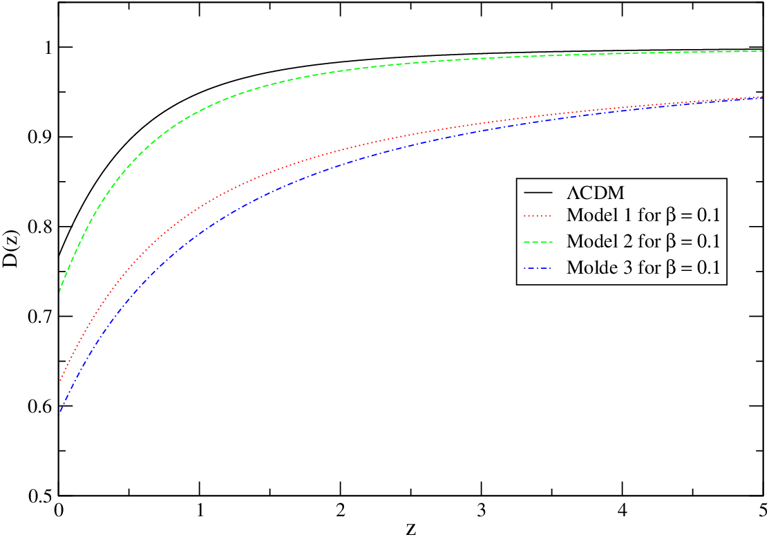
Figure 2 shows the evolution of linear perturbations of matter in terms of
for the models I, II, and III assuming . Note that the density contrast is suppressed as we increase the
rate production of matter.
The linear growth function can be parameterized of efficiently through the introduction of growth index
| (24) |
where .
This parameterization was originally introduced by Peebles [61] and then by Wang and Steinhardt [62], and it was shown to provide an excellent fit corresponding to various general relativistic cosmological models for specific values of . We will use 11 data points reported in [63], to estimate the model parameters by minimizing the quantity
| (25) |
where and the set of free parameters, and the error observed in 1.
Figure 3 and 4 shows the confidence regions at 1 and 2 for model I, and models II and III,
respectively. We note with best fits for Model I, and .
For models II (III) we note that and . The upper and lower values
represent the errors at 1. During the statistical analysis we assumed for model I,
and for models II and III. These are the boundaries for the parameter imposed by thermodynamics [18].


The real space galaxy power spectrum is related to the matter power spectrum as follows, , where is the bias factor between galaxy and matter distributions. The matter power spectrum is defined as
| (26) |
where is the Fourier transform of the matter density perturbation, defined as
| (27) |
To calculate the power spectrum of galaxies of the models presented in this paper, we modified the program
developed by E. Komatsu [60] that calculate the spherically-averaged power spectrum. Results on the
clustering of 282.068 galaxies in the Baryon Oscillation Spectroscopic Survey (BOSS) show that at large scales,
the bias factor and measured in = 2.00 0.07 [64]. We use this value to calculate the power spectrum
for the models presented.


We compared the theoretical prediction for the power spectrum of galaxy with the data of
BOSS DR11 [65]. Figure 5 show the result for model I. Again, we see that the density contrast
suppression as we increase the rate production of matter (high values of ),
when compared to the CDM. Figure 6 shows the power spectrum
for the models II (left panel) and for the model III (right panel).
IV.2 Non-linear effects
The growth of inhomogeneities on small scale are highly non-linear, with density contrast of approximately
for . Galaxies form at redshifts of the order of 2-6; clusters of galaxies form in
redshifts the order of 1, and superclusters are forming just now, then the nonlinear effects are important for
understanding the universe at the level of clusters and superclusters of galaxies.
On larger scales than 100 Mpc, where collapse is yet to come, the cosmological theory of linear disturbances can be used directly. On small scales, the only safe way to perform calculations beyond the capacity of the linear theory and through numerical simulations. Analytical approaches can offer insights very useful for investigating the nonlinear stage of the inhomogeneities. Jeong and Komatsu [66], proposed an approximation in third order of perturbation (3PT) for the nonlinear matter power spectrum as following
| (28) |
where is a suitably normalized linear growth factor (which is proportional to the scale factor during the matter era), is the linear power spectrum at an arbitrary initial time, , at which is normalized to unity, and and are both correction to the density (matter) power spectrum. [66, 67]. This is an attractive approach, as it provides the exact calculation in the quasi linear regime where the perturbative expansion is still valid. Other approaches as Halo Model [68] and HKLM Scaling Model [69] are calibrated using numerical simulations with a specific set of cosmological parameters, and thus cannot be easily extended to other cosmological models, such as dynamical dark energy models. A disadvantage of the 3PT is that its validity is limited to the quasi linear regime, and thus the result on very small scales cannot be trusted. Thus, under this approach we apply this method to investigate the effects of nonlinear matter clustering for models with creation of matter.

Let us now calculate the evolution of nonlinear power spectrum as a function of redshift, . This is related to derivatives of the density power spectrum, , as
| (29) |

As for the linear matter power spectrum during the matter-dominated era,
vanishes for this case, as expected. When the universe is dominated
by ’dark energy’, the first term is still negative but becomes smaller than the second term, yielding
. On the other hand, the Eq. (28)
shows that nonlinear evolution gives a term in which goes as ,
and thus one obtains non-zero even during the matter-dominated era.
The sign is opposite, .
Figure 7 shows at h (left panel)
and h (right panel) as a function of for the model I. The black, red, and green
line represent 0.025, 0.05, and 0.1, respectively.
Note that the presence of matter creation at small scales decreases the effects nonlinears, where
we see clearly the change in the sign of at a moderate redshift
when there is not or there is a small production of particles ().
This regime is quite nonlinear (for ).
Recall that the linear evolution due to ’dark energy’ gives a positive contribution
to , while the nonlinear
evolution gives a negative contribution to .
Figure 8 and 9 shows at h
and h as a function of for the models II and III, respectively. Thus as in the
figure 7, the black, red, and green lines represent 0.025, 0.05, and 0.1, respectively.
Note that the both models (II and III), the regime is quite nonlinear already at h, i.e, for this models
the rate of production particles not much affect the evolution of nonlinear power spectrum. Therefore,
these models have a similar dynamic for the evolution of power spectrum when compared to the CDM model.
In this section, we can see that models where the dynamics associated with the production of particles is given by a . e.g., model I, there is a great suppression in the density contrast as we increase the rate production of matter. This becomes clear when analyzing the consequences in the power spectrum. On the other hand, a dynamic model for , e.g, model II and III, makes the evolution of perturbations of matter has a very reasonable behavior, i.e, similar to the model CDM.

V Lensing-RS power spectrum
Let us now illustrate the phenomenology described above for scenarios with matter creation,
by computing explicitly the bispectrum signal as a function of the multipole described at detail in the section 2.
On small multipole, the corresponding
scales are outside the horizon, in linear regime, and . On the other hand, on sufficiently large multipoles,
probes sub-horizon scales where the nonlinear regime dominates, and it has negative sign. The transition is
located at the angular scale where the contributions from the scales in linear and nonlinear regime balance in the
integrand, so that is zero.
As mentioned previously, the essential ingredient of the lensing-RS bispectrum is the lensing-RS cross-power spectrum,
, defined by Eq. (12). With computed, we are able
to calculate the theoretical prediction of for models of matter creation.
The sign of is determined by the balance of two competing contributions:
the decaying of the gravitational potential fluctuations as and the amplification due to
nonlinear growth. Both of these are sensitive to the cosmological parameters, we thus expect is also.
The scale at which changes sign depends crucially on the scale at which the nonlinear growth overcomes
the linear effect, making the the lensing-RS bispectrum sensitive to cosmological parameters governing the growth
of structure. We are interested in measuring the effects of creation of particles (characterized by ) on the
lensing-RS bispectrum, so we fix some parameters. Fixed parameters for all analyzed cases: = 70 km/s/Mpc,
, , , , and .


Figure 10 shows computed from Eq. (12) for the model I. Where the black, red, green, and blue lines,
represents CDM (), and = 0.025, 0.05 and 0.1, respectively.
Note that the scale at which the nonlinear growth overcomes the linear effects occurs at smaller scales,
when compared with CDM. More specifically, the sign change in lensing-RS cross-power
spectrum happens at for CDM, and at , , ,
for = 0.025, 0.05 and 0.1, respectively for the CCDM model.
Figure 11 and 12, shows the effects for the models II and III, respectively. For the model II (III)
the sign change in lensing-RS cross-power spectrum happens at (), (),
(), for = 0.025, 0.05
and 0.1, respectively. Note that, thus as for the model I, for the model III
the transition is located at very small scale angular. The model II, display small variations
when compared as the CDM model.
The effects of the presence of matter creation is clear on lensing-RS bispectrum. Showing us that the scale where the nonlinear growth overcomes the linear effect depends strongly of particles creation rate . We did not address here how much this effect is robust against variations in the other cosmological parameters, but the shift caused in the lensing-RS bispectrum, due to the presence of matter creation is very clear. In summary, the effects of the parameters on the lensing-RS bispectrum will go depend of dynamic associated with .

VI Conclusions
Understand the consequences of a particular physical mechanism, or cosmological model, on the process of structure formation is an essential ingredient in
the search of a physical model that describes the observable universe.
Cosmological models driven by the gravitational adiabatic particle production have been intensively
investigated as a viable alternative to the CDM cosmology [1, 20]. Recently, Nunes and Pavon
[36] explored the possibility that the EoS determined by recent observations [23, 29] is in reality an effective EoS that
results from adding the negative EoS, (associated to the particle production pressure from the gravitational field acting on the vacuum)
to the EoS of the vacuum itself, . In the present paper, we investigate the
the implications of a continuous matter creation processes
on structure formation in large and small scales, assuming three parametric models for the particle
production rate given by Eq’s. (18-20).
We show as the matter creation affect the evolution of the perturbations of the matter the light of linear power spectrum of galaxy,
and by a approximation in third order of perturbation to the nonlinear matter power spectrum.
Note that when the dynamics associated with the particles prodution rate is given by a , model I for example,
there is a great suppression in the density contrast as we increase the rate production of matter.
When dynamic models are considered, models II and III,
they are not observed large deviations in compared to theoretical prediction of CDM model. We have shown
via lensing-RS cross-power spectrum that the scale where the nonlinear growth overcomes
the linear effect depends strongly of particles creation rate, this is, with the dynamic nature associated the .
Obviously, phenomenological models of particle production different from the ones essayed here are also worth exploring. More important, however, is to determine the rate using quantum field theory, but, as said above, this does not seem feasible until the nature of DM particles is found. Thus, hopefully through the development here performed within the context process of structure formation, help clarify the dynamic nature associated with the cosmological creation of particles.
Acknowledgements.
R.C.N. acknowledges financial support from CAPES Scholarship Box 13222/13-9. The author is also very grateful to the anonymous referee for comments which improved the manuscript considerably.References
- [1] Ya. Zeldovich, Sov. Astron. Lett. 7, 332 1981.
- [2] M. S. Turner, Phys. Rev. D, 28 1243, 1983.
- [3] J. D. Barrow, Phys. Lett., 180B, 355, 1986.
- [4] N. Turok, Phys. Rev. Lett., 60, 549 (1988).
- [5] A. A. Starobinsky, Phys. Lett. B 91, 99 (1980).
- [6] Rafael C. Nunes, Int. J. Mod. Phys. D 25 (2016) 1650067, arXiv:1603.05302 [gr-qc].
- [7] Jaume de Haro, Jaume Amoros, and Supriya Pan, Phys.Rev. D 93 (2016) 084018, arXiv:1601.08175 [gr-qc].
- [8] I. Brevik and A.V. Timoshkin, Sov. Phys. JETP 149 (2016) 786-791, arXiv:1509.06995 [gr-qc].
- [9] Varun Sahni and Salman Habib, Phys. Rev. Lett. 81 1766-1769 (1998), arXiv:hep-ph/9808204.
- [10] S. Desai and N. J. Poplawski, Phys. Lett. B 755, 183 (2016).
- [11] I. Prigogine, J. Geheniau, E. Gunzig, and P. Nardone, Gen. Rel. Grav. 21, 767 (1989).
- [12] L. A. S. Lima, J. F. Jesus, and F. A. Oliveira, JCAP 11, 027 (2010).
- [13] N. Komatsu and S. Kimura, Phys. Rev. D 89, 123501 (2014).
- [14] T. Harko, Phys. Rev. D 90, 044067 (2014).
- [15] C. Fabris, J. A. F. Pacheco and O. F. Piattella, J. Cosmol. Astropart. Phys. 06 038 (2014)
- [16] R. O. Ramos, M. V. dos Santos, and I. Waga, Phys. Rev. D 89, 083524 (2014).
- [17] I. Baranov and J. A. S. Lima, Phys. Lett. B 751 (2015) 338-342, arXiv:1505.02743 [gr-qc].
- [18] Rafael C. Nunes and Supriya Pan, Mon. Not. Roy. Astron. Soc. 459 (2016) 673-682, arXiv:1603.02573 [gr-qc].
- [19] T. Harko, F. S. N. Lobo, J. P. Mimoso, and D. Pavon, Eur. Phys. J. C 75 (2015) 386, arXiv:1508.02511 [gr-qc].
- [20] S. Chakraborty, S. Pan, and S. Saha, Phys. Lett. B 738 (2014) 424-427, arXiv:1411.0941 [gr-qc].
- [21] I. Baranov, J. F. Jesus, and J. A. S. Lima, arXiv:1605.04857 [astro-ph.CO].
- [22] S. Pan, B. K. Pal, S. Pramanik, arXiv:1606.04097 [gr-qc].
- [23] P.A.R. Ade et al., [Planck Collaboration], “Planck 2013 results. XVI. Cosmological parameters”, Astron.& Astrophys. (in the press), arXiv:1303.5076[astro-ph.CO].
- [24] A. Rest et al., “Cosmological constraints from measurements of type Ia supernovae discovered during the first years of the Pan-STARRS1 Survey”, Astrophys. J. (in press), arXiv:1310.3828[astro-ph.CO].
- [25] J.-Q. Xia, H. Li, and X. Zhang, Phys. Rev. D 88, 063501 (2013).
- [26] C. Cheng, and Q.-G Huang, Phys. Rev. D 89, 043003 (2014).
- [27] D.L. Shafer and D. Huterer, Phsy. Rev. D 89, 063510 (2014).
- [28] A. Conley et al., Astrophys. J. Suppl. Ser. 192, 1 (2011).
- [29] D. Scolnic et al., “Systematic uncertainties associated with the cosmological analysis of the first Pan-STARRS1 type Ia supernova sample”, Astrophys. J. (in the press), arXiv:1310.3824[astro-ph.CO].
- [30] R.R. Caldwell, Phys. Lett. B 545, 23 (2002).
- [31] S.M. Carroll, M. Hoffman and M. Trodden, Phys. Rev. D 68, 023509 (2003).
- [32] J.M. Cline, S. Jeon and G. D. Moore, Phys. Rev. D 70, 86 043543 (2004).
- [33] S.D.H. Hsu, A. Jenkins, and M.B. Wise, Phys. Lett. B 597, 270 (2004).
- [34] F. Sbisa, “Classical and quantum ghosts”, arXiv:14.06.4550.
- [35] M. Dabrowski, “Puzzles of the dark energy in the universe - phantom”, arXiv: 1411.2827.
- [36] R. C. Nunes and D. Pavón, Phys. Rev. D 91, 063526 (2015), arXiv:1503.04113 [gr-qc].
- [37] W. Hu and M. White, Phys. Rev. D 56, 596 (1997).
- [38] M. Rees and D. W. Sciama, Nature 217, 511 (1968).
- [39] W. Hu, Phys. Rev. D 62, 043007 (2000).
- [40] L. Verde and D. N. Spergel, Phys. Rev. D 65, 043007 (2002).
- [41] E. Komatsu and D. N. Spergel, Phys. Rev. D 63, 063002 (2001).
- [42] D. M. Goldberg and D. N. Spergel, Phys. Rev. D 59, 103002 (1999).
- [43] D. N. Spergel and D. M. Goldberg, Phys. Rev. D 59, 103001 (1999).
- [44] Fabio Giovi et al. Phys. Rev. D 71, 103009 (2004).
- [45] L. Parker, Fund. Cosm. Phys. 7, 201 (1982); L. Parker, Phys. Rev. Lett., 21, 562 (1968); L. Parker, Phys. Rev. Lett. 183, 1057 (1966); S.A. Fulling, L. Parker, and B.L. Hu, Phys. Rev. D, 10, 3905 (1974); L. Parker, Phys. Rev. D 17, 933 (1978); N.J. Paspatamatiou, and L. Parker, Phys. Rev. D 19, 2283 (1979).
- [46] L.E. Parker and D.J. Toms, Quantum Field Theory in Curved Spacetime: Quantized Fields and Gravity (Cambridge University Press, Cambridge, 2009).
- [47] J.A.S. Lima, M.O. Calvão, and I. Waga, “Cosmology, Thermodynamics and Matter Creation”, in Frontier Physics, Essays in Honor of Jayme Tiomno (World Scientific, Singapore, 1990); M.O. Calvão, J.A.S. Lima, and I. Waga, Phys. Letter. A 162, 223 (1992); J.A.S. Lima, A.S.M. Germano, and L.R.W. Abramo, Phys. Rev. D 53, 4287 (1996).
- [48] W. Zimdahl and D. Pavón, Mon. Not. R. Astron. Soc. 266, 872 (1994).
- [49] W. Zimdahl, D.J. Schwarz, A.B. Balakin, and D. Pavón, Phys. Rev. D 64, 063501, (2001).
- [50] J. Triginer, W. Zimdahl, and D. Pavón, Class. Quantum Grav. 13, 403 (1996).
- [51] J.A.S. Lima and I. Baranov, Phys. Rev. D 90, 043515 (2014).
- [52] J. Ellis, S. Kalara, K.A. Olive, C. Wetterich, Phys. Lett. B 228, 264 (1989).
- [53] P.J.E. Peebles and B. Ratra, Rev. Mod. Phys. 75, 559 (2003).
- [54] K. Hagiwara et al. [Particle Data Group], Phys. Rev. D. 66, 010001(R) (2002).
- [55] R. R. R. Reis, Phys. Rev. D 67, 087301 (2003).
- [56] O. Ramos et al., Phys. Rev. D 89, 083524 (2014).
- [57] E. V. Linder and A. Jenkins, Mon. Not. Roy. Astron. Soc. 346 573 (2003) .
- [58] Linder, E.V., 1988, Max-Planck-Institut (MPA) Research Note; Linder, E.V., 1997, First Principles of Cosmology(Addison-Wesley).
- [59] E. Komatsu et al., Astrophys. J. Suppl. 180, 330-376, (2009).
- [60] http://www.mpa-garching.mpg.de/ komatsu/.
- [61] P. J. E. Peebles, Principles of Physical Cosmology (Princeton University Press, Princeton, 1993).
- [62] L. M. Wang and P. J. Steinhardt, Astrophys. J. 508, 483 (1998).
- [63] H. T. C. M Souza et al., arXiv:1406.1706 (2014).
- [64] S. E. Nuza et al., Mon. Not. Roy. Astron. Soc. 432, 743-760 (2013).
- [65] https://www.sdss3.org/science/boss-publications.php
- [66] D. Jeong and E. Komatsu, Astrophys. J. 651, 619-626, (2006).
- [67] Jai-chan Hwang et al., JCAP05 055 (2015).
- [68] R. E. Smith, J. A. Peacock, A. Jenkins, S. D. M. White,C. S. Frenk, F. R. Pearce, P. A. Thomas, G. Efstathiou, and H. M. P. Couchman, MNRAS 341, 1311 (2003).
- [69] A. J. S. Hamilton, P. Kumar, E. Lu, and A. Matthews, Astrophys. J. Lett. 374, L1 (1991).