Baryogenesis in the two doublet and inert singlet extension of the Standard Model

The original Lagrangian with the most general potential, kinetic term, and the universally aligned Yukawa sector has 27 real parameters (not counting the parameters entering the Yukawa-flavour-mixing matrices). We removed the four arbitrary parameters from kinetic terms and three from the complex Yukawa coefficients $C_{i}$ by the use of the GL(2,$\mathbbm{C}$) invariance of the theory. This still leaves us with 15 real couplings and five real mass parameters in the model potential $V(H_{1},H_{2},S)$. Our next task is to find out which sets of these parameters correspond to physically viable models with a stable potential.

We can use the reparametrization invariance to our advantage in constructing the stable potentials. To this end, it is convenient to rephrase the invariance in terms of Lorentz invariance of the potential, written in terms of bilinears formed from hyperdoublets. Following the analysis of Ref. [19, 20, 21], we define

The bilinear four-vector $r^{\mu}$ is positive definite³³ 3 Clearly $r_{0}=\sum_{i}|H_{i}|^{2}\geq 0$. Also $r_{\mu}r^{\mu}=4(|H_{1}|^{2}|H_{2}|^{2}-(H_{1}^{\dagger}H_{2})(H_{2}^{\dagger}H_{1}))\geq 0$ , by Schwartz inequality.. That is, $r^{\mu}$ vectors span the future light cone, LC⁺, of a Minkowski space. Thus, in bilinear representation the elliptic and hyperbolic SL(2,$\mathbbm{C}$) basis transformations of fields $\Phi\rightarrow\Phi^{\prime}\equiv P\Phi$ correspond to proper orthochronous Lorentz transformations $r^{\mu}Ê\rightarrow r^{\prime\mu}={(\Lambda_{\scriptscriptstyle P})^{\mu}}_{\nu}r^{\nu}$, where ${(\Lambda_{\scriptscriptstyle P})^{\mu}}_{\nu}\in{\rm SO}(1,3)^{+}$. In this notation one can rewrite the Higgs potential (2) in a very compact form:

where we defined mass and coupling four-vectors

and a symmetric coupling tensor

where the subscripts $R$ and $I$ refer to the real and imaginary parts of the couplings, respectively. The reparametrization invariance is manifest in Eq. (7), because $V$ depends only on Lorentz-invariant products of vectors and tensors. This form is particularly suitable for a study of the vacuum stability and phase-transition patterns of the model.

First consider the direction $S=0$ in the potential (7). Here the term $r^{\mu}\lambda_{\mu\nu}r^{\nu}$ must be bounded from below. In [19] it was shown that this is the case precisely when $\lambda_{\mu\nu}$ is positive definite in the future light cone. That is, all stable potentials can be written as $\lambda_{\mu\nu}Ê\equiv{\Lambda_{\mu}}^{\alpha}\lambda^{\scriptscriptstyle D}_{\alpha\beta}{\Lambda^{\beta}}_{\nu}$, where ${\Lambda_{\mu}}^{\alpha}$ is an SO(1,3)⁺ transformation and

Note that the four parameters in $\lambda^{\scriptscriptstyle D}_{\alpha\beta}$ together with the six parameters in ${\Lambda^{\beta}}_{\nu}$ add up to the ten real degrees of freedom in the most general 2HDM potential. Second, if we set $r^{\mu}=0$ ($H_{1}=H_{2}=0$), we see that we must have

Finally, we have to consider the directions where both $S$ and $H_{i}$ are nonzero. First, if the vector $\lambda_{S\mu}$ of couplings which mix $S$ and $H_{i}$ lies in the future light cone, $\lambda_{S\mu}\in\mathrm{LC}^{+}$, i.e.

then the mixing term ${\textstyle\frac{1}{4}}\lambda_{S\mu}r^{\mu}S^{2}$ in the potential, Eq. (7), is always positive, and no new conditions arise. However, if $\lambda_{S\mu}\notin\mathrm{LC}^{+}$, there are always directions $r^{\mu}\in\mathrm{LC}^{+}$ along which the product $\lambda_{S\mu}r^{\mu}$ is negative. If we in such cases rewrite the quartic part of the potential as

we see that the potential is most negative as a function of $S$ along direction $2\lambda_{S}S^{2}=-\lambda_{S\mu}r^{\mu}$. In this subspace, the potential reduces to the form 4$V_{\rm quartic}=r^{\mu}\lambda^{\scriptscriptstyle S}_{\mu\nu}r^{\nu}$, with a new coupling matrix:

The matrix $\lambda^{\scriptscriptstyle S}_{\mu\nu}$ is not in general diagonalizable by an SO$(1,3)^{+}$ rotation, and it may have also complex eigenvalues. Unfortunately we cannot restrict its properties like we did for $\lambda_{\mu\nu}$, because $\lambda^{\scriptscriptstyle S}_{\mu\nu}$ does not need not be positive definite in the entire future light cone, but only in the subset of $\mathrm{LC}^{+}$ where $\lambda_{S\mu}r^{\mu}$ is negative. Instead of covering the full range of possibilities, we will require a sufficient (but not necessary) condition that $\lambda^{S}_{\mu\nu}$ is positive definite in the future light cone whenever $\lambda_{S\mu}\notin\mathrm{LC}^{+}$.

We now have the recipe to construct the space of stable potentials: we first choose a $\lambda^{\scriptscriptstyle D}_{\alpha\alpha}$ which satisfies Eqs. (10). Then we generate a vector $\lambda^{\scriptscriptstyle D}_{S\mu}$ and check if it satisfies the positivity constraint (12), or if the matrix $\lambda^{\scriptscriptstyle S}_{\mu\nu}$ in Eq. (14) is positive definite in the subset of LC⁺ where $\lambda_{S\mu}r^{\mu}<0$. Having found an acceptable set, we generate a random Lorentz transformation and define

where ${\Lambda^{\mu}}_{\nu}\in{\rm SO}(1,3)^{+}$.

Let us comment on the role of the kinetic and Yukawa terms in the above construction of the potential. We implicitly assumed that kinetic term becomes diagonal, and the Yukawa term becomes of type-I form in the final frame, after the Lorentz transformation. Thus, they necessarily must be nontrivial in the original, diagonal frame. Indeed, the six degrees of freedom “missing$"$ in the diagonal potential are in this frame evenly divided between the $C_{i}$ coefficients in the Yukawa Lagrangian and the mixing parameters in the kinetic term, which in the bilinear notation can be written as

Here $K_{\mu}$ is some positive definite, but otherwise arbitrary four-vector of unit length (here $\alpha$ refers to the usual space-time indices and $\mu$ to potential indices)⁴⁴ 4 In the most general case $K_{\mu}$ has four free parameters, but one parameter is here assumed to be removed by a dilatation, used to bring the length of $K_{\mu}$ to unity.. It is amusing to see that exactly a Lorentz boost (a hyperbolic SL(2,$\mathbbm{C}$) transformation on fields) is needed to bring an arbitrary $K_{\mu}$ into the canonical form: $K_{\mu}\rightarrow(1;0,0,0)$, after which the kinetic term is manifestly invariant under Lorentz rotations (elliptic SL(2,$\mathbbm{C}$) transformations on fields). These boosts and rotations into the canonical frame activate the whole ${\rm SO}(1,3)^{+}$ group discussed above and thus create all physically viable Lagrangians with bounded potentials.

Since we are interested in the cases where the singlet scalar $S$ is a DM candidate, we restrict our considerations to the cases where the potential is unbroken in S direction and hence $Z_{2}$ symmetric at low temperatures. However, to enhance the strength of the latter phase transition, we also need the $S$ symmetry to be broken at high temperatures before the symmetry breaks in the doublet direction. To this end, we must have negative quadratic term in the $S$ direction in the potential ($m_{S}^{2}>0$). This implies that there may be other minima away from the $\langle S\rangle=0$ vacuum, and we must check that none of these minima is the global one at zero temperature. The extremization conditions are:

and

Eqs. (18) are complex, so we have five equations relating vacuum fields to the parameters of the theory. Our goal is to have an unbroken singlet and a broken neutral doublet vacuum at zero temperature. In [19] it was shown that the neutral and charged vacua cannot coexist in the pure 2HDM case. When $S=0$, our potential reduces to the pure 2HDM case, and so the above statement applies here as well. Therefore, if we find a neutral vacuum, we know it is the global one in the doublet space and the charged extremum may at best be a saddle point. Moreover, even with $S\neq 0$, the doublet-symmetry-breaking pattern is formally similar to the pure 2HDM case, only with an effective mass parameter

This implies that also any neutral minimum with $S$ breaking is the lowest one in the doublet space.

The most general neutral vacuum in 2HDM field space is given by

Of course the local $\mathrm{SU}(2)$-gauge invariance guarantees that only the relative phase $\theta\equiv\theta_{2}-\theta_{1}$ is physical, and one could rotate for example $\theta_{1}\rightarrow 0$. Explicitly we find that this corresponds to

so that $r_{0}^{2}=0$ as it should for a neutral vacuum [19]. This construction actually only ensures that the special point (20) is an extremum of the potential. To check that this extremum is a also a minimum, one needs to compute second derivative matrices of the potential corresponding to scalar field masses and require that there are no negative eigenvalues. For the mass of the physical excitation in the singlet direction, this corresponds to requiring that

where the left hand side is evaluated at the extremum $\langle S\rangle=0$ and $\langle H_{i}\rangle\neq 0$ as defined in Eq. (20). These requirements on the spectrum allow one to set the Lagrangian mass parameters in terms of physical masses and vacuum expectation values (vevs) of the fields. However, it still remains to check that the vacuum with $S=0$ is the global minimum for any given set of parameters. It is straightforward to show that the value of the potential at the desired $\langle S\rangle=0,\langle H_{i}\rangle\neq 0$ vacuum is

In the direction $H_{i}=0$, the potential has at least a directional minimum at $\langle S\rangle^{2}=m_{S}^{2}/2\lambda_{S}$, and the value of the potential in this directional minimum is

We impose the condition that the minimum in Eq. (23) is below that in Eq. (24). Finally, there is an extremum where both $\langle S\rangle\neq 0$ and $\langle H_{i}\rangle\neq 0$, but this is a local maximum.

In addition to the massive scalar $S$, the physical spectrum contains the usual states arising from the two Higgs doublets: the three neutral scalars $h_{0}$, $H_{0}$ and $A_{0}$, and two charged scalars $H^{\pm}$. The diagonalization of the mass matrices is presented in detail in Appendix A. The lightest neutral scalar state $h_{0}$ is identified with the 125 GeV Higgs particle observed LHC, while the masses of the heavier neutral and charged scalar states are constrained to lie above the current limits.

The final ingredient we need for our analysis is the effective potential at finite temperature. Here we only consider the leading corrections to the potential, which bring about the symmetry restoration at high temperatures. In the high-temperature limit, these corrections are accounted for by the thermal masses:

where ($a=1,2,12,S$):

and

is the common SM contribution from the SU(2)_L and U(1)_Y gauge fields and the top quark.

The couplings between scalar fields tend to run strongly, which typically leads to a relatively low cut-off scale for the validity of the effective theory. To be specific, we demand that our model is consistent up to $\Lambda=1.5$ TeV, i.e. we check that the vacuum is stable and that all couplings remain perturbative⁵⁵ 5 For perturbativity we use the upper limit $(4\pi)^{2}$ on all scalar couplings. Over large portion of our data points the couplings will remain small also at larger scales $\mu\gg\Lambda$; the value 1.5 TeV is chosen for concreteness. up to $\Lambda$. The 1-loop renormalization-group equations needed for this calculation are summarized in Appendix B. Moreover, at zero temperature we impose

and check that this choice gives the global minimum of the potential as detailed in previous section.

Second, we address the current experimental constraints. We only accept points that give a light scalar of mass $m_{h_{0}}=125$ GeV, and for which the heavy scalars satisfy the mass limits from direct searches at LEP on charged particles, $m_{H^{+}}>500$ GeV [22], and at LHC on heavy neutral scalars, $m_{H_{0}},m_{A_{0}}>600$ GeV [23]. For consistency, we also constrain the heavy scalar masses to be below the cut-off $\Lambda=1.5$ TeV. We also take into account the electroweak precision data using the $S$ and $T$ parameters [24]. The necessary formulae for computing $S$ and $T$ can be extracted from [25], where the oblique parameters have been calculated for models with extra doublets and extra singlets. The current values of $S$ and $T$ parameters are $S=0.00\pm 0.08$, $T=0.05\pm 0.07$ with a correlation factor $\rho=0.90$ [26]. We accept points that lie within the $2\sigma$ region in the $(S,T)$ plane.

Moreover we take into account constraints on the Higgs boson couplings to SM particles using the signal-strength data from the LHC and Tevatron experiments [27, 28, 29]. First, we impose the constraint from the invisible width of the Higgs boson from LHC at $2\sigma$ level:

which here implies $\Gamma_{h_{0}\to SS}\;\raisebox{-3.00003pt}{$\stackrel{{\scriptstyle\displaystyle<}}{{\sim}}$}\;1.0$ MeV. Second, we allow for modifications to the Higgs couplings and parametrize the deviations from the SM with parameters $a_{f}$ and $a_{V}$,

We accept points which are within $2\sigma$ from the best fit values

which we obtain by performing a $\chi^{2}$ fit to the Higgs boson signal strength data. We have neglected the imaginary part of $a_{f}$ and the $h_{0}H^{+}H^{-}$ coupling in the fit, since we have checked that these couplings are very small⁶⁶ 6 As a comparison, we have performed the $\chi^{2}$ fit of $a_{f}$ and $a_{V}$ with maximum values of the imaginary part of $a_{f}$ and $h_{0}H^{+}H^{-}$ coupling for out data points, and we find that the best-fit value does not change significantly..

We compute the relic abundance of the $S$ bosons for all models passing the experimental constraints described above. We assume that $S$ is a thermal relic, i.e. we assume that at least some the portal couplings $\lambda_{S1}$, $\lambda_{S2}$ and $\lambda_{S12}$ are sufficiently large (larger than about $10^{-7}$ [30]). We then apply the standard freeze-out formalism [31], employing the accurate approximation scheme introduced in [32]. The relevant annihilation channels of our WIMP candidate are

Cross-sections for all these processes are given in a very compact form in Appendix C. To treat cases where $S$ is a subdominant DM candidate, we define the ratio [33]

which expresses how large fraction of the observed DM abundance is in form of $S$ bosons. All annihilation channels are directly proportional to the couplings between the $S$ boson and the Higgs fields, although the precise dependence is rather complicated (see Appendix C). Since the relic abundance is roughly proportional to the inverse of the annihilation cross section, large (small) couplings corresponds to a small (large) relic abundance.

Direct search limits for $S$ follow from the bound on the spin-independent cross section for $S$ scattering off nucleons. It is given by

where $m_{N}=0.939$ GeV is the nucleon mass, $\mu=m_{N}M_{S}/(m_{N}+M_{S})$ is the reduced mass of the nucleon–scalar system, and $f_{N}\approx 0.30$ [32] gives the strength of the Higgs–nucleon coupling: $g_{h_{0}N\bar{N}}=f_{N}m_{N}/v_{0}$. Finally, the effective $SSh_{0}$ coupling is given by

where $\beta$ is the vacuum mixing angle and $\theta$ the phase between the doublet vevs, and $R_{N_{ij}}$ are the components of the $4\times 4$-mixing matrix between the neutral scalar fields given in Eq. (62).

Currently the most stringent limit for $\sigma_{\mathrm{SI}}$ come from the LUX experiment [34]. However, in the case of a subdominant DM, the LUX bound is not directly related to $\sigma_{\mathrm{SI}}$ shown in Eq. (34). Instead, assuming that all DM components cluster similarly, the actual signal strength from $S$ bosons is suppressed by the fraction $f_{\rm rel}$. The relevant quantity to compare with the LUX limit then is

We show the effect of this limit on the models passing all experimental bounds on Fig. 1. Note that the scatter in $\sigma_{\rm eff}$ as a function of $m_{S}$ is much larger here than in the singlet extension of the SM [33]. Note how also the models with relatively low abundance are constrained by the LUX data.

One of the necessary conditions for a successful baryogenesis scenario is the departure from thermal equilibrium. In EWBG this is provided by a strong first-order phase transition. In pure 2HDMs, with only leading thermal corrections (i.e. with thermal masses), the phase transition is of second order. While full one-loop effects may induce a first-order transition, it still tends to be rather weak [8, 9]. In a model with a singlet scalar, a strong transition may take place with just the leading corrections (25), given a specific two-step symmetry-breaking pattern [35]. This means that, when passing from high towards low temperatures, a minimum of the potential is generated first along the singlet direction. At lower temperature, then, the potential develops a minimum where the doublets have non-zero vevs while the singlet symmetry is restored, $(\langle h_{1}\rangle,\langle h_{2}\rangle;\langle s\rangle)=(0,0;0)\rightarrow(0,0;w(T))\rightarrow(v_{1}(T),v_{2}(T);0)$, ensuing the actual electroweak phase transition. This pattern of minima should of course develop in such a way that the true ground state at $T=0$ is given by Eq. (28).

Including the thermal mass corrections of Eq. (25) to the potential, we find the transition temperatures. In particular the electroweak transition temperature, $T_{c}$, where the two minima are degenerate is determined by

where $w_{c}=w(T_{c})$ and $v_{ic}=v_{i}(T_{c})$. To determine when the transition is strong enough, we require, as usual, that

where $v_{c}=\sqrt{v_{1c}^{2}+v_{2c}^{2}}$. It turns out not to be possible to have simultaneously strong transition and dominant DM candidate in the model with $f_{\rm rel}\approx 1$. This is because having a strong transition requires that at least some of the mixing couplings $\lambda_{Si}$ are large. However, as we noted above, large mixing introduces large annihilation cross sections for $S$ bosons and hence small relic abundances. Qualitatively the behaviour is the same as in the pure singlet model [33, 32]: a strong first-order EWPT and large $f_{\rm{rel}}\approx 1$ are realized in different portions of the parameter space.

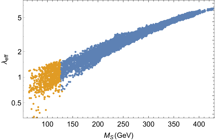
Left panel of Fig. 2 shows the correlation between the DM particle mass $M_{S}$ and the effective coupling $\lambda_{\rm{eff}}$ for models with strong EWPT. Accepted values of $\lambda_{\rm eff}$ increase as a function of $M_{S}$ because both quantities are linearly proportional to the mixing couplings $\lambda_{Si}$. Right panel of Fig. 2 shows the correlation between $M_{S}$ and the relative relic abundance $f_{{\rm rel}}$ for the same set. Note that for $M_{S}$ between the Higgs resonance and $M_{W}$, both a strong transition and a relatively large DM abundance, $f_{\rm rel}\approx 0.15$ could be obtained, but this region is now excluded by LUX.

The fact that LUX most strongly constrains models with small $\lambda_{\rm eff}$ is because $f_{\rm rel}$ is roughly inversely proportional to the square of $\lambda_{\rm eff}$, and this to large extent cancels the direct $\lambda_{\rm eff}$ dependence in $\sigma_{\mathrm{SI}}$. Larger mass region beyond the Higgs resonance is less constrained because the DM-number density falls with increasing mass.

The non-observation of electric dipole moments (EDMs) of electrons, neutrons and atoms gives stringent bounds on CP-violating interactions in multi-Higgs models. As shown in [36], currently the most stringent bound for 2HDMs arises from the electron EDM, for which the ACME experiment gives an upper limit

with $90\%$ confidence level [37]. We calculate $d_{e}$ for the points which give a strong first-order EWPT using the results from Ref. [38], where Barr–Zee type contributions to fermionic EDM were calculated in 2HDM. These results are directly applicable here as well, because the singlet scalar $S$ does not directly couple to gauge fields. In Fig. 3, we show the distribution of models passing all previous cuts as a function of $d_{e}$ and the neutral scalar mixing matrix element $R_{N_{42}}$, which expresses the projection of $h_{0}$ to complex part of the second doublet:

$\sin\Delta_{\rm CP}$ is given in terms of the various mixing angles in Eq. (62). The red region is excluded by the electron EDM constraint. Small $d_{e}$ naturally correlates with small $\sin\Delta_{\rm CP}$, because the size of $\sin\Delta_{\rm CP}$ is proportional to the size of the CP-violating mixing in the model.

The actual baryogenesis mechanism in our model relies on CP-violating interactions of the top quark with the expanding phase-transition walls. The CP violation comes directly from the spatial evolution of the complex phases of the Higgs field $H_{2}$, which renders the top mass a complex-valued function of the spatial coordinate across the wall. The first step for us is then to work out the evolution of the scalar fields over the bubble wall.

We shall approximate the true phase-transition-wall profile in the usual way, by the stationary path that extremizes the Euclidean one-dimensional action

between two degenerate minima at critical temperature $T=T_{c}$, for which the condition (37) holds. The covariant derivatives involve the classical $Z_{\mu}$ field: $D_{\mu}=\partial_{\mu}-ig/(2\cos\theta_{\rm W})Z_{\mu}$. We write the neutral components of the doublets as $h_{j}e^{i\varphi_{j}}$ and observe that the effective potential can depend only on the relative phase $\varphi\equiv\varphi_{1}-\varphi_{2}$. Following Ref. [8], we work in the gauge $Z_{\mu}=0$, whereby we need to account for four fields: $h_{1},h_{2},S$ and $\varphi$, while solving the path. The relevant reduced action is

The invariance of the potential under the change of the total phase $\varphi_{1}+\varphi_{2}$ implies a conservation law, which in the $Z_{\mu}=0$ gauge allows us to work out the phase $\varphi_{2}$ in terms of the relative phase $\varphi$ [8]:

The complex, spatially-varying top mass can now be constructed from the phase $\varphi_{2}(x)$ and the modulus $h_{2}(z)$:

In fact, one does not need to solve for the top phase, since only its derivative, given by Eq. (43), appears in the source term for the diffusion equations for chemical potentials:

Here $\xi_{w}$ is the wall velocity, primes denote $\partial_{zT}$ and $K_{n,t}$ are dimensionless functions of $x_{t}\equiv|m_{t}|/T$ arising from phase-space averaging of certain kinematic variables defined in [39].

Given the source, one can calculate chemical potentials $\mu_{j}(z)$ for top, bottom, anti-top and Higgs by solving a set of transport equations defined in [7]. Finally the baryon-to-entropy ratio $\eta_{B}\equiv n_{B}/s$ is given by

We take $\xi_{w}=0.1$ for the wall velocity and $g_{*}=106.75$ for the number of degrees of freedom in the plasma. The left-chiral baryon chemical potential is

For the sphaleron rate we use a formula interpolating between the symmetric and the broken phase [8],

where $v(z)^{2}=h_{1}(z)^{2}+h_{2}(z)^{2}$.

In the left panel of Fig. 4 we show how the baryon-to-entropy ratio relative to the observed value $\eta_{B}^{\rm obs}=8.7\times 10^{-11}$ [40] correlates with the CP-violation-sensitive parameter $\sin\Delta_{\rm CP}$ defined in (40). Shown are only the points which survive the eEDM bound. As expected, the size of $\sin\Delta_{\rm CP}$ correlates with the size of $\eta_{B}$. This trend is similar to the correlation between $\sin\Delta_{\rm CP}$ and $d_{e}$ shown in Fig. 3. However, a large $\eta_{B}$ does not always imply a large $d_{e}$, as is clear from the right panel of Fig. 4, where we show the correlation between $d_{e}$ and $\eta_{B}$, again for points that pass the EDM bound. Apparently, while both quantities are sensitive to the CP-violating parameters in the model, they can be sensitive to different linear combinations of them, so that large $\eta_{B}$ may be obtained simultaneously with a small enough $d_{e}$.

Fig. 5 shows the distributions of various physical parameters in our parametric scan. Orange colour refers to models that pass all experimental cuts described in Secs. 3.1 and 3.2, and give a strong EWPT, blue to models that in addition satisfy EDM constraint and green to models which also give large baryon-to-entropy ratio $\eta_{B}/\eta_{B}^{\rm obs}\in[0.5,2]$. These plots must be interpreted with care, since our scans were partly tuned by hand. Nevertheless, we see that none of the vevs can be very large and in particular both $v_{1}$ and $v_{2}$ need to be nonzero. Also the critical temperature is bounded from above: $T_{c}\;\raisebox{-3.00003pt}{$\stackrel{{\scriptstyle\displaystyle<}}{{\sim}}$}\;100$ GeV. Finally for the models with large $\eta_{B}$, the new scalar masses are in general bound from above: $m_{H},m_{A_{0}},m_{H^{\pm}}\;\raisebox{-3.00003pt}{$\stackrel{{\scriptstyle\displaystyle<}}{{\sim}}$}\;1.4$ TeV and $m_{S}\;\raisebox{-3.00003pt}{$\stackrel{{\scriptstyle\displaystyle<}}{{\sim}}$}\;400$ GeV, which is encouraging from the point of view of experimental verifiability of the model.

So far we have implicitly assumed that the bubble nucleation takes place at a temperature not too different from the critical temperature. This is typically the case in models where the first-order phase transition is effected by cubic corrections to potential from infrared modes, which leads to rather mild supercooling and small latent heat release. Here the situation is different, because the barrier between the degenerate minima is essentially due to a tree-level term. Thus a stronger supercooling and more latent heat release may be expected, or even a possibility of a formation of a metastable vacuum where the electroweak breaking never takes place.

We study the nucleation problem in the thin-wall limit [41]. The bubble nucleation rate is given by

where $S_{3}(T)$ is the three-dimensional action for an O(3)-symmetric bubble. In the thin-wall limit, it is given by

where $\Delta V(T)$ is the potential energy difference between the electroweak-symmetric and electroweak-broken minima and $\sigma$ is the surface tension,

integrated along the path from the symmetric to the broken minimum at temperature $T=T_{c}$. The bubble nucleation temperature $T_{n}$ is defined as the temperature at which creating at least one bubble per horizon volume is of order one. This condition can be written as

We show the results of the nucleation-temperature calculation for our data set on the left panel of Fig. 6. Obviously, a large number of points displayed in Fig. 4 are missing in Fig. 6. The reason is that for these models, indicated by red dots in Fig. 4, no solution to Eq. (52) was found. In these cases, in the thin-wall approximation, the fields were trapped in the false vacuum. Moreover, of the surviving models only four give large $\eta_{B}$.

The situation is actually more dire than this: another implicit assumption in our baryon asymmetry calculation is that the transition walls are subsonic deflagrations, which is required for efficient diffusion of particle asymmetries across the bubble wall. However, with a large latent heat release the walls tend to be supersonic detonations instead. A full microscopic analysis of wall dynamics including a computation of the wall friction is beyond the scope of this paper. However, a deflagration wall must necessarily satisfy a condition [42]

where $\rho(T_{n})$ is the radiation energy density in the symmetric phase. We show this condition in the right panel of Fig. 6 (blue dots) for the set of models shown in the left panel. As expected, for the models with the lowest nucleation temperatures, deflagrations are not possible. This applies in particular to all four surviving models with a large baryon-to-entropy ratio.

There are two issues that ameliorate the situation. First, the validity of the thin-wall limit actually requires a small latent heat and/or a large surface tension, which is often not the case here. When not applicable, thin-wall limit tends to overestimate the action $S_{3}(T)$, and hence underestimate the nucleation rate and eventually $T_{n}$. Accurate calculation of the nucleation rate is quite complicated in the full model, however, and we do not pursue it here. Instead, we compare the nucleation temperatures found in the thin-wall limit and in the full calculation in the simpler, singlet extension of the SM, studied for example in [33, 32]. In practice we minimize the action

where $h$ is the SM-Higgs field, and $V_{\rm SSM}(h,S,T)$ is the singlet-model potential.

The results of this analysis are shown in Fig. 7. The blue dots show the nucleation temperature in the thin-wall approximation and the yellow dots the same quantity found from the solving minimizing the action (54) . As expected, the thin-wall approximation underestimates nucleation temperatures significantly. We find that the true nucleation temperature $T_{n}$ and the thin-wall value $T_{n}^{\rm tw}$ are related by $T_{n}=T_{c}-\kappa\,(T_{c}-T_{n}^{\rm tw})$, where the coefficient $\kappa$ to some extent depends on $M_{S}$ and $\lambda_{S}$, but is less than $0.7$. We anticipated this result in the deflagration limit shown in the right panel of Fig. 6, where the yellow dots were found by redefining all thin-wall nucleation temperatures by the above equation with $\kappa=0.7$. We believe that this scaling conservatively represents the effect of going beyond thin-wall approximation in the full 2HDM and singlet model, and hence shows that most parameter sets may in fact be deflagrations.

We can also tune our search to prefer models with a higher critical temperatures. Indeed, as is clearly seen from Fig. 7, the nucleation temperature approaches the critical temperature when $T_{c}$ gets higher in the singlet extension of the SM and this feature persists also in the full 2HDSM. Hence, we made a new parametric scan, where we accept only models with $T_{c}>80$ GeV. The result of this scan is seen in Fig. 8, where the left panel again shows the baryon-to-entropy ratio and in the right panel the deflagration bound. We now found more points with large asymmetry and, in particular after one rescales the thin-wall nucleation temperatures as explained above, these points are now well below the deflagration bound Eq. (53).

References

- (1) N. Turok and J. Zadrozny, Electroweak baryogenesis in the two doublet model, Nucl. Phys. B358 (1991) 471–493.
- (2) N. Turok and J. Zadrozny, Phase transitions in the two doublet model, Nucl. Phys. B369 (1992) 729–742.
- (3) K. Funakubo, A. Kakuto, and K. Takenaga, The Effective potential of electroweak theory with two massless Higgs doublets at finite temperature, Prog. Theor. Phys. 91 (1994) 341–352, [hep-ph/9310267].
- (4) A. T. Davies, C. D. Froggatt, G. Jenkins, and R. G. Moorhouse, Baryogenesis constraints on two Higgs doublet models, Phys. Lett. B336 (1994) 464–470.
- (5) J. M. Cline, K. Kainulainen, and A. P. Vischer, Dynamics of two Higgs doublet CP violation and baryogenesis at the electroweak phase transition, Phys. Rev. D54 (1996) 2451–2472, [hep-ph/9506284].
- (6) M. Laine and K. Rummukainen, Two Higgs doublet dynamics at the electroweak phase transition: A Nonperturbative study, Nucl. Phys. B597 (2001) 23–69, [hep-lat/0009025].
- (7) L. Fromme, S. J. Huber, and M. Seniuch, Baryogenesis in the two-Higgs doublet model, JHEP 11 (2006) 038, [hep-ph/0605242].
- (8) J. M. Cline, K. Kainulainen, and M. Trott, Electroweak Baryogenesis in Two Higgs Doublet Models and B meson anomalies, JHEP 11 (2011) 089, [arXiv:1107.3559].
- (9) G. C. Dorsch, S. J. Huber, and J. M. No, A strong electroweak phase transition in the 2HDM after LHC8, JHEP 10 (2013) 029, [arXiv:1305.6610].
- (10) A. Pich and P. Tuzon, Yukawa Alignment in the Two-Higgs-Doublet Model, Phys. Rev. D80 (2009) 091702, [arXiv:0908.1554].
- (11) E. H. Simmons, Phenomenology of a Technicolor Model With Heavy Scalar Doublet, Nucl. Phys. B312 (1989) 253–268.
- (12) A. Kagan and S. Samuel, Renormalization group aspects of bosonic technicolor, Phys. Lett. B270 (1991) 37–44.
- (13) M. Antola, M. Heikinheimo, F. Sannino, and K. Tuominen, Unnatural Origin of Fermion Masses for Technicolor, JHEP 03 (2010) 050, [arXiv:0910.3681].
- (14) T. Alanne, S. Di Chiara, and K. Tuominen, LHC Data and Aspects of New Physics, JHEP 01 (2014) 041, [arXiv:1303.3615].
- (15) M. Geller, S. Bar-Shalom, and A. Soni, Hybrid dynamical electroweak symmetry breaking with heavy quarks and the 125 GeV Higgs boson, Phys. Rev. D89 (2014), no. 3 035012, [arXiv:1302.2915].
- (16) M. Hashimoto and V. A. Miransky, Dynamical electroweak symmetry breaking with superheavy quarks and 2+1 composite Higgs model, Phys. Rev. D81 (2010) 055014, [arXiv:0912.4453].
- (17) H. S. Fukano and K. Tuominen, A hybrid 4 generation: Technicolor with top-seesaw, Phys. Rev. D85 (2012) 095025, [arXiv:1202.6296].
- (18) H. S. Fukano and K. Tuominen, 126 GeV Higgs boson in the top-seesaw model, JHEP 09 (2013) 021, [arXiv:1306.0205].
- (19) I. Ivanov, Minkowski space structure of the Higgs potential in 2HDM, Phys.Rev. D75 (2007) 035001, [hep-ph/0609018].
- (20) I. P. Ivanov, Minkowski space structure of the Higgs potential in 2HDM. II. Minima, symmetries, and topology, Phys.Rev. D77 (2008) 015017, [arXiv:0710.3490].
- (21) I. Ivanov, Thermal evolution of the ground state of the most general 2HDM, Acta Phys.Polon. B40 (2009) 2789–2807, [arXiv:0812.4984].
- (22) ALEPH Collaboration, A. Heister et al., Search for charged Higgs bosons in collisions at energies up to = 209-GeV, Phys. Lett. B543 (2002) 1–13, [hep-ex/0207054].
- (23) ATLAS Collaboration, G. Aad et al., Combined search for the Standard Model Higgs boson in collisions at TeV with the ATLAS detector, Phys. Rev. D86 (2012) 032003, [arXiv:1207.0319].
- (24) M. E. Peskin and T. Takeuchi, A New constraint on a strongly interacting Higgs sector, Phys.Rev.Lett. 65 (1990) 964–967.
- (25) W. Grimus, L. Lavoura, O. Ogreid, and P. Osland, The Oblique parameters in multi-Higgs-doublet models, Nucl.Phys. B801 (2008) 81–96, [arXiv:0802.4353].
- (26) Particle Data Group Collaboration, K. A. Olive et al., Review of Particle Physics, Chin. Phys. C38 (2014) 090001.
- (27) CDF, D0 Collaboration, T. Aaltonen et al., Higgs Boson Studies at the Tevatron, Phys. Rev. D88 (2013), no. 5 052014, [arXiv:1303.6346].
- (28) CMS Collaboration, V. Khachatryan et al., Precise determination of the mass of the Higgs boson and tests of compatibility of its couplings with the standard model predictions using proton collisions at 7 and 8 TeV, Eur. Phys. J. C75 (2015), no. 5 212, [arXiv:1412.8662].
- (29) ATLAS Collaboration, G. Aad et al., Measurements of the Higgs boson production and decay rates and coupling strengths using pp collision data at and 8 TeV in the ATLAS experiment, Eur. Phys. J. C76 (2016), no. 1 6, [arXiv:1507.04548].
- (30) K. Kainulainen, S. Nurmi, T. Tenkanen, K. Tuominen, and V. Vaskonen, Isocurvature Constraints on Portal Couplings, JCAP 1606 (2016), no. 06 022, [arXiv:1601.07733].
- (31) P. Gondolo and G. Gelmini, Cosmic abundances of stable particles: Improved analysis, Nucl.Phys. B360 (1991) 145–179.
- (32) J. M. Cline, K. Kainulainen, P. Scott, and C. Weniger, Update on scalar singlet dark matter, arXiv:1306.4710.
- (33) J. M. Cline and K. Kainulainen, Electroweak baryogenesis and dark matter from a singlet Higgs, JCAP 1301 (2013) 012, [arXiv:1210.4196].
- (34) LUX Collaboration, D. S. Akerib et al., Improved Limits on Scattering of Weakly Interacting Massive Particles from Reanalysis of 2013 LUX Data, Phys. Rev. Lett. 116 (2016), no. 16 161301, [arXiv:1512.03506].
- (35) J. R. Espinosa, T. Konstandin, and F. Riva, Strong Electroweak Phase Transitions in the Standard Model with a Singlet, Nucl. Phys. B854 (2012) 592–630, [arXiv:1107.5441].
- (36) S. Inoue, M. J. Ramsey-Musolf, and Y. Zhang, CP-violating phenomenology of flavor conserving two Higgs doublet models, Phys. Rev. D89 (2014), no. 11 115023, [arXiv:1403.4257].
- (37) ACME Collaboration, J. Baron et al., Order of Magnitude Smaller Limit on the Electric Dipole Moment of the Electron, Science 343 (2014) 269–272, [arXiv:1310.7534].
- (38) T. Abe, J. Hisano, T. Kitahara, and K. Tobioka, Gauge invariant Barr-Zee type contributions to fermionic EDMs in the two-Higgs doublet models, JHEP 01 (2014) 106, [arXiv:1311.4704]. [Erratum: JHEP04,161(2016)].
- (39) L. Fromme and S. J. Huber, Top transport in electroweak baryogenesis, JHEP 03 (2007) 049, [hep-ph/0604159].
- (40) Planck Collaboration, P. A. R. Ade et al., Planck 2015 results. XIII. Cosmological parameters, arXiv:1502.01589.
- (41) A. D. Linde, Decay of the False Vacuum at Finite Temperature, Nucl. Phys. B216 (1983) 421. [Erratum: Nucl. Phys.B223,544(1983)].
- (42) J. R. Espinosa, T. Konstandin, J. M. No, and G. Servant, Energy Budget of Cosmological First-order Phase Transitions, JCAP 1006 (2010) 028, [arXiv:1004.4187].
- (43) A. Degee and I. Ivanov, Higgs masses of the general 2HDM in the Minkowski-space formalism, Phys.Rev. D81 (2010) 015012, [arXiv:0910.4492].