Density of Spherically-Embedded Stiefel and Grassmann CodesThanks: ©2017 IEEE. Personal use of this material is permitted. Permission from IEEE must be obtained for all other uses, in any current or future media, including reprinting/republishing this material for advertising or promotional purposes, creating new collective works, for resale or redistribution to servers or lists, or reuse of any copyrighted component of this work in other works. This work was supported in part by the Academy of Finland (grants #276031 and #299916) and by the Nokia Foundation. Part of this work was presented at the 2011 IEEE International Symposium on Information Theory and the 2012 Asilomar Conference of the Signals, Systems and Computers. R.-A. Pitaval was with the Department of Communications and Networking, Aalto University, FI-00076 Espoo, Finland. He is now with Huawei Technologies Sweden AB, SE-164 94 Kista, Sweden (e-mail: renaud-alexandre.pitaval@alumni.aalto.fi). L. Wei is with the Department of Electrical and Computer Engineering, University of Michigan-Dearborn, Michigan 48128, USA (e-mail: luwe@umich.edu). O. Tirkkonen is with the Department of Communications and Networking, Aalto University, FI-00076 Espoo, Finland (email: olav.tirkkonen@aalto.fi). C. Hollanti is with the Department of Mathematics and Systems Analysis, P.O. BOX 11100, FI-00076 AALTO, Finland (email: camilla.hollanti@aalto.fi).
Abstract
The density of a code is the fraction of the coding space covered by packing balls centered around the codewords. A high density indicates that a code performs well when used as a uniform point-wise discretization of an ambient space. This paper investigates the density of codes in the complex Stiefel and Grassmann manifolds equipped with the chordal distance arising from an Euclidean embedding, including the unitary group as a special case. The choice of distance enables the treatment of the manifolds as subspaces of Euclidean hyperspheres. In this geometry, the densest packings are not necessarily equivalent to maximum-minimum-distance codes. Computing a code’s density follows from computing: i) the normalized volume of a metric ball and ii) the kissing radius, the radius of the largest balls one can pack around the codewords without overlapping. First, the normalized volume of a metric ball is evaluated by asymptotic approximations. The volume of a small ball can be well-approximated by the volume of a locally-equivalent tangential ball. In order to properly normalize this approximation, the precise volumes of the manifolds induced by their spherical embedding are computed. For larger balls, a hyperspherical cap approximation is used, which is justified by a volume comparison theorem showing that the normalized volume of a ball in the Stiefel or Grassmann manifold is asymptotically equal to the normalized volume of a ball in its embedding sphere as the dimension grows to infinity. Then, bounds on the kissing radius are derived alongside corresponding bounds on the density. Unlike spherical codes or codes in flat spaces, the kissing radius of Grassmann or Stiefel codes cannot be exactly determined from its minimum distance. It is nonetheless possible to derive bounds on density as functions of the minimum distance. Stiefel and Grassmann codes have larger density than their image spherical codes when dimensions tend to infinity. Finally, the bounds on density lead to refinements of the standard Hamming bounds for Stiefel and Grassmann codes.
Index Terms:
Unitary matrix codes, spherical codes, Grassmann manifold, Stiefel manifold, density, packing, metric ball, volume, Hamming bound.I Introduction
Sphere packing is a classical problem with a long history from geometry to information theory [1, 2, 3, 4]. In his 1948 seminal work [5], Shannon made the connection between the capacity of an additive white Gaussian noise channel and packing of multidimensional spheres. This interpretation was later generalized to non-coherent multi-antenna channels and packings in products of Grassmann manifolds [6].
Stiefel and Grassmann codes are matrix codes with applications to Multiple Input Multiple Output (MIMO) communications [7, 6, 8, 9], Code Division Multiple Access (CDMA) wireless systems [10], and compressive sensing [11, 12]. The complex Stiefel manifold is the space of rectangular semi-unitary matrices. The Grassmann manifold is the space of eigenspaces spanned by the Stiefel matrices. An element in the Grassmann manifold is an equivalence class of Stiefel matrices, which can be alternatively represented by a unique projection matrix. When discussing codes in Grassmann manifolds of one-dimensional subspaces, the equivalent language of frame theory is often used [12].
Depending of the application and convenience, several non-equivalent distances can be defined on these spaces [13, 14]. A common distance for the unitary group and Stiefel manifold is simply the Frobenius norm of the difference of two matrices [15]. Similarly for the Grassman manifold, an often-used distance arises from the Frobenius norm of the difference between two projection matrices [8, 16]. These distances correspond to embed the manifolds into Euclidean spaces. Through these embeddings, each manifold is a subset of an hypersphere and the distance is the length of a chord.
For the application of limited-feedback MIMO precoding, unitary precoder designs have been reduced to quantization problems on Grassmann and Stiefel manifolds with the associated chordal distance [8, 17, 9]. In the context of space-time coding, the code performance in the low signal-to-noise-ratio (SNR) regime has also been related to the chordal distance [18, 16]. More recently, analogical results have been derived for linear classification: In the small model mismatch regime, the number of classes that can be distinguished by a subspace classifier is governed by the chordal distance among subspaces, and more generally by their principal angles [19].
In the last decade, basic coding-theoretic results estimating the relationship between the cardinality and the minimum distance of codes in Grassmann and Stiefel manifolds have been published [20, 21, 22, 23, 24, 15, 25, 17, 26, 27]. The standard Hamming bound relates the minimum distance to the notion of code density. The density of a code is the maximum portion of the coding space covered by non-intersecting balls of equal radius. In classical geometry, maximizing the code’s density is known to be equivalent to maximizing its minimum distance. For the Stiefel and Grassmann codes measured by chordal distance, this equivalence does not always hold.
The present paper investigates this surprising fact and discusses the density of codes in Grassmann and Stiefel manifolds equipped with their chordal distance. We provide a direct connection between minimum distance and density via lower and upper bounds on the density for a given distance. This connection leads to new conjectured bounds on the minimum distance as a function of code cardinality. Related to applications, numerical evaluations suggest that the density may be a more relevant criterion for MIMO precoding than the minimum distance. While for space-time coding, the minimum distance of a code may be more important than its density.
There are two main difficulties in evaluating the density of codes in these spaces: 1) evaluating the normalized volume of a ball, and 2) estimating the kissing radius of codes.
The problem of estimating the volume of a metric ball has been addressed in [28, 20, 22, 23, 17, 29, 26, 27]. In the large code cardinality regime, balls are small and can be approximated to be balls in flat space. While some exact evaluations were obtained in Grassmannian cases [28, 17], the case of the Stiefel manifold has been less addressed. A powerful and general framework is provided in [22, 26, 27]. However, it appears that the state-of-the-art volumes in the literature do not correspond to the desired metrics. Indeed, the volume element is unique up to a non-vanishing scaling factor which is often dismissed, as it can be absorbed in the overall normalization. From Nash embedding theorem [30], every Riemannian metric can be seen as induced by an appropriate Euclidean embedding. There exists an intrinsic metric locally equivalent to the chordal distance, and thus a consistent volume density that defines the notion of volume on the manifold. In this respect, we provide the exact scaling of the volume for Grassmann and Stiefel manifolds induced by the spherical embedding, leading in turn to precise small ball approximations.
For larger radius, we show that the volume of a ball in the manifold can be well approximated by the “area” of the hyperspherical cap the ball is embedded into. The approximation is supported by a volume comparison theorem showing that the normalized volume of a ball in the manifold is asymptotically equal to the normalized volume of a ball in the embedding sphere. This result generalizes and provides a structural unification of our previous results in [31, 32, 33]. The derivation is a by-product of the asymptotic Gaussianity of the chordal distance arising through its reduction to linear statistics. The intuition behind relates to a classical result by Borel [34] who proved that coordinates of a hypersphere are asymptotically Gaussian as the dimension tends to infinity [35], and the long history of central limit theorems showing the Gaussian behavior of linear statistics [36] in random matrix theory.
Next, the paper addresses the evaluation of the kissing radius and density of Grassmann and Stiefel codes. The kissing radius is the analog of the packing radius for linear codes [37], which has applications in, e.g., sphere-decoder optimization [38, 39]. It is the largest possible radius of packing balls around the codewords of a code. The kissing radius also relates to rate-distortion theory as it is the smallest possible distance from a codeword to the border of its Voronoi cell. The problem reduces to finding the minimum mid-distance between two points at a given distance . For a geodesic distance on a flat space, the answer is simply , the so-called packing radius. With a strictly extrinsic distance, the triangle inequality is never satisfied with equality and the kissing radius is greater than . While for spherical codes there is a one-to-one mapping between the kissing radius and the minimum distance, this is not always the case for the Grassmann and Stiefel codes with chordal distance. As a consequence, the density is not a single-variable function of the minimum distance of the code, and two codes with equal minimum distance could have different densities. This is in sharp contrast with classical packing problems where maximizing the density is equivalent to maximizing the minimum distance. The kissing radius and the density cannot be determined solely from the minimum distance but it is possible to derive bounds. Combining these bounds with the volume comparison theorem discussed above shows that the densities of Grassmann and Stiefel codes are asymptotically greater than or equal to the densities of their image spherical codes. The bounds are shown to be tight by simulations.
Finally, a direct application of bounds on density is to revisit the Hamming bounds. The results of this paper improve the Hamming bound for the Grassmann case in [20, 22]; and generalize the bound for the unitary group in [23] to the Stiefel manifold.
The rest of this paper is organized as follows. Section II introduces the considered spaces and their geometry. Section III states the problem and necessary definitions. Section IV addresses the problem of the volume of a ball. In Section V, bounds on kissing radius and density are derived. Section VI provides concluding remarks.
II The Grassmann and Stiefel Manifolds
We consider the following Riemann manifolds equipped with a chordal distance induced by their canonical spherical embedding. Throughout the paper, stands for the unitary group , Stiefel manifold , or Grassmann manifold embedded into the sphere of radius , or , in a Euclidean space of dimension , or , respectively. Elements in the manifold are represented by matrices in or endowed by the inner product , where is the real part and is the matrix trace. The geometric description below follows directly by generalizing [13] and [14] to the complex space. The chordal distances, the dimension of the manifolds, and the corresponding embeddings are summarized in Table I.
II-A Hypersphere
The Euclidean -sphere of radius in is defined as
| (1) |
For , we simply write . The chordal distance is the natural Euclidean distance applied to elements on the sphere. Given it is simply the norm of the difference:
| (2) |
It is an extrinsic distance as it measures the length of a chord outside of the manifold itself, which here is the surface of the sphere.
II-B Unitary Group
The unitary group is the set of unitary matrices,
| (3) |
where denotes the Hermitian conjugate. This compact Lie group is a manifold of dimension . By differentiating the unitary constraint, one can verify that the tangent space at is the set of matrices such that is skew-Hermitian. Specifically, at identity, the tangent space is the Lie algebra of skew-Hermitian matrices .
One can parametrize with reference to a fixed via skew-Hermitian matrices as with . For a fixed , the exponential map defines the geodesic between and by mapping the tangent space to the manifold as with . A Riemannian metric may be defined from the canonical embedding of in the Euclidean space , then is the matrix exponential.
Consider the eigenvalue decomposition where the diagonal elements of are non-negative and real. This decomposition is unique if these principal angles can be strictly ordered . This leads to the corresponding eigenvalue decomposition , and accordingly the geodesic between and becomes
| (4) |
The geodesic distance is the intrinsic distance between two points obtained by integrating the geodesic path along the manifold. It is given by the norm of the tangent direction according to the considered Riemannian metric
| (5) |
Alternatively, the canonical distance in the ambient matrix-space is
| (6) | |||||
where the last equality follows from the decomposition (4).
By observing that for all , one verifies that the unitary group equipped with has an isometric embedding into the sphere . The concrete embedding is obtained from the classical mapping by vectorizing a complex matrix into a real vector.
II-C Stiefel Manifold
The complex Stiefel manifold is the space of rectangular semi-unitary matrices,
| (7) |
This provides a generalization of both the hypersphere and the unitary group. For , one directly recovers , while for and by identification of with , this corresponds to the unit sphere .
As for the unitary group, the tangent space at is the set of matrices such that is skew-Hermitian. In general, tangents have the form where is skew-Hermitian, is the orthogonal complement of such that the concatenation is unitary, and is an arbitrary complex matrix. Specifically at “identity” , tangents are of the form
| (8) |
By counting the degrees of freedom in the tangent space, one finds that the Stiefel manifold is a space with dimension .
Given a starting point and a fixed tangent direction , the canonical embedding of in the Euclidean space leads to the following geodesic equation [14],
| (9) |
The geodesic distance between and is then
| (10) |
Remark 1.
To the best of our knowledge, when , unlike for the unitary group, it is not known how to compute the geodesic in closed-form, given only and .
The corresponding Euclidean/chordal distance from the ambient space is
| (11) |
Similarly as for the unitary group, one can verify that for all , and thus this gives an isometric embedding of the Stiefel manifold into .
As an alternative to (7), the Stiefel manifold can be treated as the quotient space , where a point in is an equivalence class of unitary matrices . A natural geometry in this interpretation of the Stiefel manifold is the one inherited from the geometry of the unitary group embedded in . One can split the tangent space of the unitary group at between the so-called vertical and horizontal spaces: . The vertical space is the tangent space of at corresponding to “movements” inside the equivalence class. The horizontal space is the orthogonal complement of the vertical space, providing a unique representation for tangents to the quotient space. For at , it is the collection of matrices , where and . With this non-equivalent geometry, the geodesic distance between and is The metric induced by this embedding, and the resulting volume is discussed in [27]. This metric is not further considered in this paper.
II-D Grassmann Manifold
The complex Grassmann manifold is the quotient space of over :
| (12) |
Elements in are equivalence classes of rectangular semi-unitary matrices :
| (13) |
We can identify the equivalence class with a unique matrix representation, which is desirable for pratical implementation and computation. By symmetry (c.f. the discussion in [33]) and for simplicity, we will assume for the Grassmann manifold, all along this paper.
As described above, tangent vectors at take the form . This can be again split between the vertical space and the horizontal space . At , horizontal tangents are thus of the form , and we have . Consider the compact singular value decomposition , where , and . By setting , the geodesic equation (9) for the Grassmann manifold reduces to [14]
| (14) |
The geodesic equation could be rotated from the right by any unitary matrix as it will still belong to the same equivalence class. Without loss of generality one can thus restrict the range of the singular values of to for all . These values are known as the principal angles between the planes and . Contrary to the Stiefel manifold, here given two end points and , one can compute the tangent in the geodesic (14) and satisfy by singular value decomposition of and , where the singular values of are .
The geodesic distance is given by
| (15) |
In [13], the following distance was defined
| (16) |
which is locally-equivalent to (15) as when , and corresponds to a Euclidean embedding since
| (17) | |||||
This is in fact an isometric embedding into [13] which follows from mapping any to the space of detraced Hermitian matrices as
| (18) |
and the chordal distance is the ambient Euclidean distance
| (19) |
In this ambient space of dimension , it can be further verified that the distance of any from the origin is , and thus belongs to a sphere of radius . When there is no ambiguity on the considered space, we will simply write , which is well-defined as the distance does not depend on the Stiefel representatives.
Alternatively, the Grassmann manifold can be expressed as the quotient space . In this representation, elements in a Grassmann manifold are equivalence classes of unitary matrices. The tangents of at the identity are of the form for this second quotient representation. Again, we do not consider this representation, but we note here that the natural geodesic distance induced by this embedding only differs from (15) by a scaling factor,
| (20) | |||||
III Packing Problem and Maximum Code Density
A packing is a maximal set of non-intersecting balls of fixed radius, covering the space so that it is not possible to fit in another ball. For a given code size, a packing thus gives the maximum density, i.e. the maximum fraction of the space that one can cover by non-intersecting balls. This problem is considered to be the dual of a coding problem: maximizing the code cardinality for a given minimum distance or reciprocally maximizing the minimum distance for a given code cardinality. Surprisingly, these two problems are not necessarily equivalent for the Grassmann and Stiefel manifolds with chordal distance. This is because there is not necessarily a one-to-one mapping between the minimum distance and the kissing radius of the code, which follows from the choice of an extrinsic distance combined with the two-point inhomogeneity of the spaces [40, 15].
III-A Code, Minimum Distance, and Metric Balls
An -code is a finite subset of elements in ,
| (21) |
where is the minimum distance defined as
| (22) |
A metric ball of radius with center is the subset
| (23) |
III-B Kissing Radius
Given a code, one can surround each codeword by metric balls of the same radius and enlarge them until two balls touch. This leads to the notion of kissing radius. The kissing radius is a generalization of the so-called packing radius. We choose a different terminology to emphasize here that the kissing radius of a code may not be a function of the minimum distance, and also because the packing radius is sometimes defined as irrelevantly of the choice of distance [41] by extension from flat geometry.
Definition 1.
The kissing radius of a code is the maximum radius of non-overlapping metric balls centered at the codewords:
| (24) |
For each codeword pair , there exists a mid-point which is the closest equidistant point satisfying subject to . The mid-points define the mid-distances , and the kissing radius is the minimum of all of them .
As the chordal distance is measured along a geodesic defined by the associated Riemann metric, the midpoints can be computed accordingly: with the geodesic such that and , the midpoint is . In the case of the unitary group and the Grassmann manifold, the geodesic equation is fully parametrized by a set of principal angles as given in (4) and (14), respectively, and the mid-distance can then be directly computed from half of these angles . However, for the case of the Stiefel manifold, the geodesic equation between two points is not known as explained in Remark 1. Alternatively, the midpoint can be computed11 1 Except if and are antipodal then their center of mass is which does not have a unique projection. by an orthogonal projection of the center of mass , which for the Stiefel manifold is given by polar decomposition [9].
For spherical codes one has only one principal angle. This results in a one-to-one mapping between the minimum distance and kissing radius. In contrast, for the Grassmann and Stiefel manifolds with chordal distance, the kissing radius and the minimum distance may not be directly expressible as functions of each other. First, the kissing radius corresponds to the mid-distance between two codewords, which may not be at the minimum distance from each other. Second, for a given pairwise distance, one may have different mid-distances. Grassmann and Stiefel manifolds are not in general two-point homogeneous spaces [40, 15]: one cannot necessarily find a unitary mapping between two pairs of equidistant points, i.e., a pair cannot always be mapped to a pair even if . In fact, in the case of and , the collection of principal angles provides the complete relative position between two points which is transitive under the action of the unitary group. However, by compressing this “vector-like distance” to the scalar distance , one loses transitivity.
III-C Density
The density of a code is the fraction of covered by metric balls centered around the codewords with radius equal to the kissing radius. We consider a uniform measure on inherited from the Haar measure on the unitary group. Recall that the Grassmann and Stiefel manifolds are homogeneous spaces of the unitary group. For any measurable set and any , the uniform measure satisfies . Due to the homogeneity of , the characteristics of this ball are independent of its center which for convenience will often not be specified. The measure corresponds to a normalized volume
| (25) |
satisfying .
Definition 2.
The density of a code is defined as
| (26) | |||||
| density | density |
| min. dist. | min. dist. |
| kissing radius | kissing radius |
| where |
| Cardinality | Cardinality |
| min. dist. | min. dist. |
| kissing radius | kissing radius |
By definition, it satisfies . A maximum packing code has the maximum density for a given cardinality. The problem of maximizing the density for a given cardinality corresponds to maximizing the kissing radius of the code. This could be in fact reformulated as another maximum-minimum distance problem where distances among codewords would be defined by the mid-distances. In the case of the Grassmann manifold and unitary group, this would correspond to halve the principal angles in the chordal distance definition, which for the Grassmann manifold can be identified as the “chordal Frobenius-norm” [14] (up to a scaling factor).
In general, the packing problem is not necessarily equivalent to maximizing the minimum distance of the code, and codes with same minimum distance may also have different kissing radiuses and thus densities. We illustrate these statements with two concrete examples below. The first example describes two Grassmann codes where the (proven) maximum minimum-distance code has a lower density than another code.
Example 1.
Consider the two Grassmannian codes given in Table II. The density of these codes of cardinality four in is according to the volume formula provided in [17].
The first code is an optimal max-min distance code reaching the Rankin simplex bound [1, 13], constructed by embedding the optimal tetrahedron code of [42]. The embedding is obtained by a tensor product with the identity matrix, following [43, Prop. 12]. This is a strongly simplicial configuration in the sense that all principal angles equal . The mid-distances between each pair of codewords are thus all the same, approximately , leading to a density of .
The second code is obtained by circular permutation of the rows of the truncated identity matrix. Its distance distribution corresponds to the embedding of a square. The principal angles between two codewords are either or . The mid-distances between each of the codewords are either or . The density of this code is , almost twice the density of the optimum max-min distance code while it has a smaller minimum distance.
The codes in Example 1 can be generalized to two infinite families of codes and in where both have constant minimum distance and kissing radius: Given , the codewords are constructed by the -fold tensor product for all , leading to a code with codewords in with constant minimum distance and kissing radius . The code is obtained by row permutations of the truncated identity matrix leading to codewords with constant minimum distance and kissing radius . For all , the first construction has a larger minimum distance than , but the latter has a larger kissing radius and density as summarized in Table III. The code is larger than but one could select only codewords as in without changing the kissing radius and minimum distance.
| density | density |
| min. dist. | min. dist. |
| kissing radius | kissing radius |
| Generator matrices: | Generator matrices: |
| The signs are selected such that their product is . | |
| 28 codewords obtained by circular permutation of the rows of the four generator matrices | |
The second example shows that two optimal maximal-minimum-distance codes with different densities can exist.
Example 2.
In [44], an infinite family of real Grassmann codes meeting the Rankin simplex bound is described generalizing a code found in [13]. Since the simplex bound is the same for real and complex Grassmannians, these codes are also maximum-minimum-distance complex Grassmann codes. It is observed that this construction can lead to different codes with same minimum distance but a different distribution of principal angles, and thus different densities. This observation follows from the lowest dimensional examples and in Table IV. Each code is the union of four orbits under the action of the cyclic group but from different generator matrices. The density of these codes of cardinality 28 in can be approximated [17] to . The code has three distinct sets of principal angles and thus three distinct mid-distances from which the kissing radius is . The code has two distinct sets of principal angles and thus two mid-distances, among which the set of angles with mid-distance is also a mid-distance of . The kissing radius is achieved with the other set of principal angles which has a mid-distance only slightly smaller (it does not seem to have a compact form). While both codes reach the optimal minimum distance of , the code has a density about 5 times larger than .
We briefly discuss the performance of these codes when applied to MIMO communications.
MIMO precoding is well-known to be related to Grassmannian packing [8]. In this context, the mutual information with Gaussian signaling is given by where is the per-stream SNR, and is a quantization map that selects the codeword index in maximizing the instantaneous rate for each channel realization inside the expectation. Entries of are assumed to be standard complex normal variables . Numerical evaluations of corresponding mutual informations for the codes in Examples 1 and 2 show that the two higher density codes and slightly outperform the codes and , respectively. provides a SNR gain of dB over , and provides a SNR gain of dB over , in the SNR region dB. These examples and other numerical experiments hint that it may be in fact the density of the code that primarily governs the achievable rate of transmission rather than the maximum-minimum distance. We believe this behavior to be quite generic for the following reason. MIMO precoding reduces to a quantization problem on the Grassmann manifold with chordal distance [17], and the mid-distances of the code reflect better the rate-distortion trade-off since they represent the first border effects of the Voronoi cells.
We now look at the application of unitary codes as space-time constellations over a non-coherent MIMO transmission . Here and have standard complex normal entries, and is uniformly selected from the code . The standard approach in this case is to design Grassmann codes that maximize the product diversity since it is minimizing the pairwise block error rate at high-SNR [45]. Low-SNR analysis [18] shows on the other hand that it is the chordal distance (sum diversity) that dominates the block error rate, and it was additionally observed in [16] that codes maximizing the chordal distance can lead to higher mutual information than codes with high product diversity. Furthermore, subspace perturbation analysis in [46] suggests that an appropriate code metric is given by the chordal Frobenius-norm, which is exactly the kissing radius of the code with chordal distance as explained above, and thus its density. From the evaluation of the mutual informations of the codes in Examples 1 and 2 shown on Figure 1, the code density does not seem to be an ultimate performance measure when it comes to mutual information, as clearly outperforms . It should be noted that has both a higher minimum chordal distance and product diversity than , the later having zero product diversity between four codeword pairs out of six.
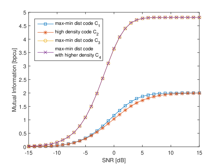
III-D Hamming Bound
The notion of density directly relates to the Hamming bound: For any -code, one must satisfy
| (27) |
The upper bound in (27) is a direct application of the standard Hamming bound to without taking into account the curvature of the space and the choice of distance. The chordal distance, inherited from a Euclidean embedding, is extrinsic to the considered curved space and thus never satisfies the triangle inequality with equality. Accordingly, balls of radius around the codewords do not necessarily form a packing, as none of the balls would be touching each other and one could possibly fit in an extra ball. The kissing radius is larger than , and the Hamming bound can be refined by any radius , and ultimately for ,
| (28) |
By construction and thus the Hamming bound (28) is always tighter than the ‘standard Hamming bound’ (27), while being asymptotically equivalent for .
The difficulty in exploiting the improved bound (28) is in finding a relationship between the kissing radius and the minimum distance of the code. To obtain a bound on the minimum distance, one needs to find a function of the minimum distance such that . Then, provided that both the volume expression and are invertible, it is possible to bound the minimum distance from above.
IV Volumes
In this section, we address the problem of volume computation in the manifolds, providing two different asymptotic approximations of the volume of balls operating in different regimes.
IV-A Spherical Volumes and Hyperspherical Caps
The - and -dimensional volume of (with its natural metric ) are respectively
| (29) |
Since the manifolds of interest are submanifolds of hyperspheres, the considered balls are subsets of hyperspherical caps. A hyperspherical cap is a ball on a sphere,
| (30) |
for some implicit center . One can define a uniform spherical measure , and the normalized volume of the spherical caps is denoted by . We use a different notation for distinction with the uniform measure on the manifold but if considering then the two measures match .
The -dimensional volume of a spherical cap can be computed exactly, as given below. It is given along with two asymptotics proven in Appendix A.
Lemma 1.
The normalized volume (area) of a hyperspherical cap in measured with chordal distance is given by
| (31) |
where is the radius of the cap satisfying , and is the regularized incomplete beta function.
As the radius of the cap goes to zero, the volume of the spherical cap tends to
| (32) |
On the other hand, as the dimension of the sphere goes to infinity with fixed, the volume tends to
| (33) |
where is the Gauss error function defined in Eq. (75).
The volume (32) equals . Intuitively, when a cap is small it is almost “flat” and its volume tends to be the “area of a disc”. The volume (33) corresponds to an asymptotic Gaussian behavior for large dimensions: the squared chordal distance of uniformly distributed random points is asymptotically Gaussian; where is the normal distribution with mean and variance . A similar expression formulating this high-dimensional regime can be found in [47, 48]. As , high-dimensional random vectors are asymptotically orthogonal and the chordal distance tends to which is the mid-distance between two antipodal points.


IV-B Manifold Volume and Small Ball Approximation
IV-B1 Overall Manifold Volume
The volume of a space can be obtained from the integration of a volume element, which is unique on a Riemannian manifold up to a non-vanishing scaling factor. This scaling factor is induced by the chosen distance, and impacts the overall volume. The theorem below provides the volumes correctly scaled for the chordal distance.
Theorem 1.
The volumes of the manifolds induced by the chordal distance (or its equivalent geodesic distance ) are
- •
for the unitary group [49]
(34) - •
for the Stiefel manifold
(35) - •
for the Grassmann manifold
(36)
A detailed volume computation is provided in Appendix B. While it is possible to find the exact volume for the unitary group rigorously derived for the chordal distance in [49, 50], the equivalent result for the Stiefel manifold does not seem to have been reported before. This volume differs by a constant factor from the commonly cited formula, see e.g. [6, 20, 22]. In many contexts, the overall scaling of the volume is meaningless as often the induced scaling would be absorbed or canceled out. The volumes known in the literature arise from integration of a volume element neglecting scalar prefactors. Conventional volumes in the literature are expressed as the product of the volumes of spheres: where is given in (29). The two different conventions are related by . For the Grassmann manifold with the geometry induced by the spherical embedding, it appears that these normalizations cancel out so that we have . However, we remark that the true volume of the Grassmannian with the quotient geometry and distance is , which differs from in the embedding geometry computed above by a factor of . Using the conventional volumes, one would get , i.e. the volumes in the two geometries would erroneously be assumed to be the same. When interpreting the Haar measure as a normalized volume (25), keeping track of the scaling of the volume is necessary. We suspect that omitting the volume scaling factors is one of the reasons behind the numerical errors observed in [22], in which a standard volume formula was used irrespectively of the geometric interpretation of the Stiefel and Grassmann manifolds, and the related distances.
IV-B2 Small Ball Approximation
The volume of a small geodesic ball can be well approximated by the volume of a ball of equal radius in the tangent space. This approximation, tight as the radius goes to zero, is actually an upper bound as discussed in [22], known as the Bishop–Gromov inequality, a volume comparison theorem valid for any Riemannian manifold. In [22], it was used to evaluate volumes of small geodesic balls in the Grassmann and Stiefel manifolds. For the case of the Stiefel manifolds, results were extended to the chordal distance in an indirect manner from the geodesic distance combined with local inequalities. Surprisingly, the results of [17] show that this approximation is exact for the Grassmann manifold with chordal distance smaller than one, in the same manner as the area of a cap of the real sphere equals the area of a disk. Later, the same approximation was used in [51] for volumes in simple flag manifolds. Refining the result, a power series expansion for the volume of small geodesic ball in any Riemannian manifold [52] was later leveraged in [26, 27]. Limiting this expansion to the leading term gives as
| (37) |
where is according to (29) with the dimension of the manifold in Table I. Intuitively, in a small neighborhood the manifold looks like a Euclidean space and can be approximated by the tangent space. Other coefficients of the series expansion are addressed in [27] requiring computation of the curvature of the manifold.
The expansion (37) given for the geodesic distance extends to the corresponding chordal distance induced by the isometric embedding in as [53, 54]. Therefore, the normalized volume of metric balls in with dimension for both the geodesic distance and the chordal distance is given by
| (38) |
as . We then have the following results as a direct consequence of Theorem 1 and given in (29).
Corollary 1.
The volume of metric balls as with metrics or is
| (39) |
- •
where for the Stiefel manifold ,
(40) - •
and for the Grassmann manifold [17],
(41)
In the case of the geodesic distance , the Bishop–Gromov inequality [22] is accordingly given by .
For the Stiefel manifold with , the result above differs from the one in [27] derived for quotient geometry (). The two results match for the unitary group with , as expected. Comparing to the Grassmannian case in [27], there is a difference by a factor of . The local equivalence between the chordal distance and the geodesic distance makes the result identical for both metrics. For the Grassmann manifold with chordal distance, the result of [17] is stronger than Corollary 1 as it gives for .
The approximated volumes in Corollary 1 for the Stiefel manifold (with ) and for the unitary group (with ) are compared with simulation in Fig. 2. The figures are shown in logarithm scales since the region of interest is small chordal distance. We see that the approximations match almost exactly the simulations as , which is a consequence of the exact volume normalization given in Theorem 1.
IV-C Complementary Balls
As an interlude, we discuss complementary balls. Small ball approximations can be used to compute the volume of very large balls almost totally covering the space. In the same manner as a sphere can be fully covered by two complementary caps satisfying
| (42) |
we have the following analogous result for the Stiefel and Grassmann manifolds, proved in Appendix C.
Lemma 2.
In the Stiefel manifold ,
| (43) |
implying that the volume is symmetrical at .
We remark that there is a structural difference here between the Stiefel and Grassmann manifolds. The antipodal on the embedding sphere to a point in the Stiefel manifold always belongs to the same Stiefel manifold. This is not always true for the Grassmann manifold except for , as the antipodal on the sphere to a point in belongs to . This observation will be useful in the interpretation of the high-dimensional regime discussed next.


IV-D Volume Comparison Theorem and Spherical-Cap Approximation
We now present a second volume approximation: For the manifolds isometrically embedded in , the uniform measure of a ball in can be well approximated by the spherical measure of a cap on . The two normalized volumes are indeed asymptotically equivalent in the high-dimensional regime. Before stating the theorem, we highlight an intermediate result of independent interest.
Lemma 3.
The squared chordal distance or drawn from a uniformly distributed random point and a reference point, say , converges in distribution to a Gaussian random variable:
| (45) |
- •
for the Stiefel manifold , as and where the finite-size regime mean and variance are given by
(46) - •
for the Grassmann manifold , as with fixed, and where
(47)
The proofs are given in Appendix D. They are obtained by reducing the chordal distances to the linear statistics of random matrix ensembles and studying their moment-generating functions. Such linear statistics are asymptotically Gaussian, and by computing the two first moments one finds the asymptotic forms. The case of the Stiefel manifold is closely related to the partition function of the von-Mises Fisher distribution, while for the Grassmann manifold it is related to the partition function of the Bingham distribution [55].
It follows that the chordal distance is well-approximated by a Gaussian random variable with the same finite-size mean and variance, i.e. for the Stiefel manifold , and for the Grassmann manifold .
Using (33) for the hypespherical cap volumes, one gets a volume comparison of the ball in the embedded manifold with the embedding spherical cap:
Theorem 2.
The normalized volume of a ball of radius in is asymptotically equal to the normalized volume of a cap with same radius in the embedding sphere ,
| (48) |
in the high-dimensional regime as given in (33). We have
- •
for the Stiefel manifold ,
(49) as with fixed;
- •
and for the Grassmann manifold ,
(50) as with and fixed.
The proof is given in Appendix E. The volume (49) generalizes our previous result [31, 32] from the unitary group to the Stiefel manifold. The volume (50) corresponds to the special case in [33]. Theorem 2 provides a geometric unification of the asymptotic expressions which are shown to be closely related due to their spherical embedding. The different asymptotic regimes for the Stiefel and Grassmann manifolds can be geometrically understood as the behaviors in Lemma 2. The Stiefel manifold fully covers all possible distances on its embedding sphere. This is not the case for the Grassmann manifold, and as a consequence and are not defined on the same support, except for . In the regime with fixed , one has and the volume expressions are then asymptotically defined on the same support.
There exists a body of literature on comparison theorems in Riemannian geometry that compares volumes among manifolds with reference to the standard sphere. However, these theorems often compare manifolds of equal dimension, e.g. the Bishop-Gromov inequality or the Berger-Kazdan comparison theorem. To the best of our knowledge, volume comparisons of these manifolds with their embedding spheres in Theorem 2 is new.
The quality of the approximation is illustrated in Figure 3. The normalized volume of metric balls for different Grassmann and Stiefel manifolds obtained via Monte Carlo simulations is compared to the normalized volume of their respective embedding hyperspherical cap, together with their joint asymptotic expression. The exact volume of the hyperspherical cap is as given by Lemma 1. This numerical evaluation shows that the three volume expressions are very close to each other even in the low dimensional regime.
V Kissing Radius and Density
In this section, we discuss the kissing radius of codes with chordal distance, and apply volume approximations derived in the previous section to evaluate code density. Recall that for the Grassmann and Stiefel manifold with chordal distance, the kissing radius cannot be directly expressed in term of the minimum distance of the code. In the following, upper and lower bounds on and the corresponding bounds on density are provided.
V-A Preliminaries
V-A1 Hypothetical Covering Radius
Ideally, a set of packing balls would fully cover the space, reaching a maximum density of one. This is only possible when the cardinality of the code is , otherwise one gets an upper bound. This ideal radius fulfills
| (51) |
Two volume approximations were discussed in the previous section. Depending of the regime, one may compute accordingly.
- •
- •
V-A2 Kissing Radius for Spherical Codes
For spherical codes with chordal distance, the kissing radius of a code is given by a one-to-one mapping from the minimum distance, directly computable by the Pythagorean theorem. Given an -spherical code on , the midpoint on the geodesic between the two codewords of distance is at distance from the extremities:
| (54) |
which can be inverted as
| (55) |
V-A3 Preliminary Bounds on Kissing Radius
Since we are considering a manifold isometrically embedded in the Euclidean sphere , an -code in is an -spherical code. As a consequence, as balls of radius are non-overlapping on , their inverse image on are also non-overlapping, and we can deduce that . On the other hand, we know that for every non-overlapping ball of radius , we have .
Lemma 4.
It should be noted here that the lower bound is a function of the minimum distance , while the upper bound is a function of the cardinality .


V-B Bounds on Kissing Radius and Density
We now provide bounds on the kissing radius as a function of the minimum distance of the code only, and corresponding bounds on code density.
Proposition 1.
For any -code in , we have
| (57) |
where
| (58) |
| (59) |
and is the smallest integer greater than . It follows, therefore, that the density is bounded by
| (60) |
A detailed proof can be found in Appendix F. Given two points either on the Grassmann manifold or the unitary group, their midpoint can be determinated according to their principal angles. The bounds then follow by optimizing over the principal angles. For the unitary group, the obtained lower bound matches the spherical lower bound in Lemma 4, and can thus be extended to any Stiefel manifold. We conjecture that the upper bound (59) can be generalized to all Stiefel manifolds. However, the lack of a closed-form geodesic equation between two points, as explained in Remark 1 (or equivalently the absence of the notion of principal angles), renders a tentative proof of generalization difficult. Nevertheless, numerical experiments support this generalization, and note that the upper bounds (59) do not depend on any dimension parameter.
For the Grassmann manifold, the lower bound in Proposition 1 provides an improvement of the spherical embedding bound (see Appendix F-D).
Corollary 2.
Figure 4 illustrates the upper and lower bounds (57) on the kissing radius and shows that is a good approximation for only when the minimum distance of the code is relatively small. In general, since the chordal distance is not strictly intrinsic, we have . The bounds are also compared to simulated midpoints between a fixed center and uniformly-distributed random points. We stress that in this case the bounds are tight in the sense that it is always possible to construct two diagonal codewords fulfilling the bounds.

V-C On High-Density Codes
Since the lower bound (58) is an increasing function of , a large minimum distance always guarantees a good code density but not necessarily the highest one.
V-C1 Numerical Experiments
Figure 5 compares the density of codes with sizes from to in to the density bounds (60) in Proposition 1. The Grassmannian is embedded in , and the corresponding spherical Rankin bound33 3 In this dimensionality, spherical codes achieve the simplex bound for , then the orthoplex bound for . provides an upper bound on the maximum possible minimum distance of Grassmannian codes. We have generated Grassmannian codes according to two criteria: a maximum-minimum-distance criterion, and a low-distortion44 4 The code distortion refers here to the average squared quantization error of a uniform random source quantized to the code. criterion. For visibility, the densities from the latter are displayed at while for the former at . For each code, two densities are displayed on Fig. 5: i) the density as a Grassmann code, and ii) the density as a spherical code. The bounds on Grassmann densities from Proposition 1 are shown as range bars. The higher is the minimum distance of the code, the higher is the bar.
Maximum-minimum-distance codes were obtained using the Alternating Projection algorithm from [41]. The obtained codes match the Rankin bound on squared minimum distance with numerical precision.
The Lloyd algorithm is used to create low-distortion codes. It is expected to provide high density codes since the kissing radius corresponds to the first border effect of Voronoi cells. In [17], it was shown that distortions are bounded by idealized codes that would have only one border effect, corresponding to a kissing radius equal to , i.e. the upper bound (56) of Lemma 4.
While the Alternating Projection algorithm generates numerically optimal simplicial codes with maximum minimum distance, their density appears to be always close to the corresponding lower bound. This means that the codes are strongly simplicial configurations where all principal angles are almost equal. Comparing to the codes generated by Lloyd algorithm, the results for cardinalities and clearly show the weak relationship between maximizing the minimum distance and maximizing the density. For , the Lloyd algorithm produced an equivalent max-min-distance code, which is at the density lower bound. For , it generated a code with smaller minimum distance but larger density, reaching the density upper bound. The configurations obtained for correspond to codes numerically equivalent to the closed form codes in Table II. For , the Lloyd algorithm produced a code with minimum distance close to the optimum, as for , but this time with a density reaching the upper bound, while the code from the Alternating Projection algorithm is close to the lower bound. For other cardinalities, the Lloyd algorithm produced codes with greater or equal density but smaller minimum distance than Alternating-Projection codes.
Lastly, an interesting characteristic of Grassmann codes is that their density for is not , except for . This comes from the fact that when one cannot have two spherically antipodal points, c.f. the symmetry of Lemma 2. For example, the density of two orthogonal lines in is equal to , and one can actually pack a third orthogonal line to reach the density of .
V-C2 Comments on Algebraic Constructions
For a given minimum distance , the proof of Proposition 1 shows that to achieve the largest density in or , a highly concentrated distribution of principal angles should be targeted where almost all non-zero principal angles should be at the maximum value which is for and for . Conversely, the lower bound is achieved when all principal angles are equal.
When constructing group codes from orbits of a symmetry group, the distribution of principal angles can be controlled. The two infinite families of codes in Table III are orbit codes. is an orbit under the action of the -fold tensor product of the projective unitary representation of the Klein 4-group [56], i.e. a direct product of the group of symmetries of a tetrahedron. As a result, the principal angles between two points at minimum distance are and the kissing radius is at the lower bound (58) of Proposition 1. The code is an orbit of the fundamental representation of the symmetric group via permutation matrices in the corresponding dimension. The resulting principal angles are either or if the two codewords have zero or one column in common, respectively. Contrary to , the codes reach the upper bound (59) of Proposition 1.
In [44], a family of optimal max-min distance Grassmann codes is presented from which the code in Example 1 is a subset of. These codes are orbits of a large Clifford group generalizing the symmetries of the square. This results in highly symmetric codes where many principal angles are . Nevertheless, the kissing radius of these codes typically does not reach the upper bound (59). Consider the half-subspaces construction in from [57, 44]. Its complex extension [16] leads to a code of codewords. Due to its orbit structure, the collection of pairwise distances or principal angles can be computed independently of the reference codeword as described in [44]. For each codeword, there is always an antipodal codeword at pairwise distance , and others at distance . The codes thus meet the Rankin orthoplex bound. Among the codewords at minimum distance from a given codeword, there are that have principal angles (each value with multiplicity ), whereas the remaining codewords have principal angles . Thus roughly half of the squared mid-distances are , and roughly the other half are . These mid-distances thus meet the upper bound (59) and lower-bound (58), respectively. The kissing radius of this code family is hence the lower bound . It should be remarked that a mid-distance at the lower bound (58), where principal angles between two codewords are equal, corresponds to maximizing the diversity product for the given chordal distance. Therefore, about half of the codeword pairs have a good product diversity of , while the others have a product diversity . The codes in [44, 16] provide thus a mixture of high chordal mid-distance (as advocated in [46] by the chordal Frobenius-norm) and high product diversity (as advocated in [45]), in addition to a high chordal distance (as advocated in [18]). This observation may provide further support to their good performance observed in [16] when applied to space-time constellations.
V-D Relation to Density of Spherical Codes.
As considered in this work, for manifolds isometrically embedded in Euclidean spheres, an -code in is also an -spherical code. The density of a code in the manifold differs from the density of its image code in the embedding sphere. Combining the asymptotic equality from Theorem 2 between volume of balls in the manifold and hyperspherical cap with the kissing radius bounds from Proposition 1, we have the following comparison.
Proposition 2.
The density of codes in the Stiefel and Grassmann manifolds are asymptotically greater than the density of their image spherical codes in the high-dimensional regime of Theorem 2. The inequality is strict for the Grassmann manifold with .
This proposition is illustrated in Figure 5 where densities of the image spherical codes of the considered Grassmann codes are also depicted. One observes that the densities of the image spherical codes are always less than the densities of the original Grassmannian codes for .
We remark also few special cases. In the case , the lower and upper bounds on the kissing radius in Proposition 1 are matching . Moreover with , the Stiefel manifold is isometric to the embedding sphere, while for the Grassmann manifold the volume of a ball has been calculated exactly in [17]. In these cases the density can be computed exactly as a function of the minimum distance.
Corollary 3.
For any packing with , on manifolds or ,
| (61) |
and
| (62) |
V-E Hamming-type Bounds
Bounds on density directly translate to Hamming-type bounds on code cardinality and minimum distance.
V-E1 Hamming Bound on Cardinality
According to Proposition 1, we have:
Corollary 4.
For any -code in , and given defined in (58),
| (63) |
V-E2 Hamming-type Bound on Minimum Distance
From the spherical embedding of the manifolds, we have the following Hamming-type bound on the minimum distance:
Lemma 5.
Given an -code in isometrically embedded in , and a satisfying (51), we have
| (64) |
This follows from a direct combination of (55) and Lemma 4. For the unitary group, a similar bound was derived in [23, Theorem 2.4]. For the Stiefel manifold, the result is new. For the Grassmann manifold, a tighter bound is provided as a by-product of Proposition 1, which is a generalization of a bound for line packing in [60] to any value of :
Lemma 6.
Given a -code in , we have
| (65) |
V-E3 Illustration and Conjectured Improvement
The standard Hamming bound (27) and the Hamming bound from the kissing radius analysis (65) are displayed in Fig. 6 for the Grassmannian as a function of the code rate. One verifies that (65) improves (27) and they are getting equivalent as . These Hamming bounds are also compared to the spherical Rankin bounds. Rankin provided three consecutive upper bounds in [1] on the number of spherical caps that can be packed for a given angular radius. The two first bounds, known as the simplex and orthoplex bounds, can be easily inverted to bound the minimum distance. However, the third bound is expressed through an integral which we numerically inverted for Fig. 6. For , the Rankin bounds are tight at the saturating value [61], i.e. at rate . For higher cardinality the Rankin bounds are not reachable. As expected, the Hamming bounds become tighter than the Rankin bounds for large code sizes.
By construction the Hamming bound is loose even if one would be able to exactly compute the kissing radius as a function of minimum distance. The manifold can never be totally covered by packing balls (except for ), and one always has a gap between and . In order to sharpen the Hamming bound one could use rather than to get a better estimate of the minimum distance. It is very likely that in general , which can be verified at the two ends of the code size spectrum and . Inverting (59) gives the following approximation,
| (67) |
which is guaranteed to be an upper bound as . This conjectured improvement is displayed for in Fig. 6. Here, is computed from (52) from [17] as in this case it is exact for any . Interestingly, it meets the Rankin orthoplex bound at , i.e. close to where this bound is saturating.

VI Conclusion
The density of Grassmann and Stiefel codes with chordal distance has been investigated. The analysis pertains to treat the codes as subclasses of spherical codes since the chordal distance induces embeddings in Euclidean hyperspheres. The investigation is motivated by an exotic behavior: in this context maximizing the density of a code is not equivalent to maximizing its minimum distance. We addressed both critical steps to compute a code’s density, which are computing the volume of balls and the kissing radius. For the volume of balls, our main results included a proper scaling of the manifold volume consistent with the chordal distance, which is needed in small ball approximation. Moreover, an asymptotic Gaussian behavior of chordal distances in the high-dimensional regime leading to an asymptotic equivalence between the volume of balls in the manifolds and the volume of caps in the embedding spheres was found. Then the kissing radius and density of codes were bounded as a function of the minimum distance of the codes. It was concluded that Stiefel and Grassmann codes have larger density than their image spherical codes in high dimensions. Finally, as a by-product of the analysis, refinements of the standard Hamming bounds for Stiefel and Grassmann codes were provided.
Appendix A Proof of Lemma 1–Hyperspherical Cap Area
A-A Proof of (31)
The area of a hyperspherical cap is given in [62] in which the radius of the cap is measured by an angle . This translates in our notation to a radius of , that gives and directly leads to
| (68) |
for .
The result further simplifies by normalizing by the overall area of the sphere and using the identity valid for [63, (8.17.6)][64]. The volume for larger radius can be computed by the complementary cap, i.e.
| (69) |
and using the identity [63, (8.17.4)][64]. Altogether, one obtains (31) for the whole range of the radius .
A-B Proof of (32) – Small Cap
We start from (68) which after normalization gives
| (70) |
Expressing the regularized incomplete beta function with the Beta function and the incomplete Beta function gives
| (71) |
From the identity [63, (8.17.7)] where is the hypergeometric function given by [63, (15.2.1)], it can be verified that as , which in turn gives
| (72) |
as .
A-C Proof of (33) – Large Dimension
The normalized volume of a cap can be interpreted as the probability that a uniformly distributed vector is at distance less than from a fixed point . Without loss of generality, we choose the center of the cap to be and express the chordal distance by where is the first coordinate of normalized by the sphere radius and scaled. Noting that
the volume is
| (73) | |||||
where is the cumulative distribution function of the random variable . Note that since the constraint is always satisfied, one has .
With , converges in distribution to a standard Gaussian random variable [34, 35], i.e.
| (74) |
where
| (75) |
is the Gauss error function. Therefore, with fixed, we have
| (76) | |||||
Finally, in order to provide a finite-size approximation that satisfies the basic property of a measure, , in addition to converging to the asymptotic form above, we use in (73) the finite-size correction which corresponds to approximating to be Gaussian also in the finite-size regime. This leads to the given expression.
Appendix B Proofs of Overall Volumes
is an -dimensional Riemann manifold with infinitesimal metric
| (77) |
in local coordinates . The volume element of is [65]
| (78) |
Now, consider the Euclidean space of complex matrices with its canonical inner product from which the Riemann metrics considered are constructed. Given we have
| (79) | |||||
Restricting the metric to the space of skew-Hermitian matrices, with we get
| (80) |
and the corresponding volume element
| (81) |
Note here that the off-diagonal elements are counted twice, leading to an overall scaling factor of . The overall volumes of the manifolds need to be scaled accordingly to be consistent with the chosen metric.
B-A Volume of Unitary Group
Given a unitary matrix , by differentiating , we obtain
| (82) |
showing that the differential form is skew-Hermitian. Due to the unitary invariance of the metric , its restriction to can be expressed in terms of the global form . Then, the infinitesimal metric is
| (83) | |||||
and the volume form in local coordinates is
| (84) |
where
| (85) |
is a common volume element normalized so that [66, 67]. Finally with the metric considered,
| (86) |
where the complex multivariate gamma function is
| (87) |
B-B Volume for Stiefel Manifold in Theorem 1
Now let and such that , i.e. the first columns of are the columns of . The differential form is “rectangular skew-Hermitian”, i.e. where is -by- skew-Hermitian. Similarly, due to unitary invariance of the metric, the volume element for the Stiefel manifold can be expressed in terms of the global form and is given in local coordinates as
| (88) |
where
| (89) |
is a common volume element normalized so that [66, 67]. Finally,
| (90) |
B-C Volume for Grassmann Manifold
The volume of the Grassmann manifold directly follows from the quotient geometry over the Stiefel manifold associated with :
| (91) |
Alternatively it can be computed from the quotient geometry over the unitary group associated with
| (92) |
where the scaling coefficient comes from the in the definition of compared to .
Appendix C Proof of Lemma 2–Complementary Balls
Stiefel Manifold
Consider the center to be . It has a unique antipodal point (i.e. a farthest possible point from ) which is and we have
| (93) |
Given a point such that , it is a direct verification that , thus implies and finally
| (94) |
Grassann Manifold
From the mapping (18), the Grasmmann manifolds and are both embedded in the same sphere . The definition of chordal distance thus directly extends between any and as
| (95) | |||||
The distance reaches its maximum at with , where the is the orthogonal complement of such that is a unitary matrix. The maximum distance is exactly twice the embedding radius, , i.e. is the antipodal of on the embedding sphere. The final result follows by the same argumentation as for the Stiefel manifold. Here the Pythagorean theorem gives .
Appendix D Proof of the asymptotic Gaussianity of the chordal distances in Lemma 3
Before proceeding the proof, we first state some useful definitions and intermediary results.
D-A The Hypergeometric Function of Complex Matrix Argument
For an Hermitian matrix , the hypergeometric function of a complex matrix argument is defined as [68, 69]
| (96) |
where denotes a partition of integer into no more than parts, i.e. with , the sum is over all partitions, and
| (97) |
is the multivariate hypergeometric coefficient [68, Eq. (84)]. In (96), denotes a zonal polynomial [68, 69], which is a homogenous symmetric polynomial of degree in the eigenvalues of . Denoting the -th eigenvalue of by , the zonal polynomial can be represented as [68, Eq. (85)],
| (98) |
where
| (99) |
and
| (100) |
is a Schur polynomial55 5 When some eigenvalues of are equal, the corresponding Schur polynomials (100) are obtained by using l’Hospital’s rule.. Schur polynomials form a basis in the space of homogeneous symmetric polynomials in variables of degree for all . In particular, we have [68, Eq. (17)]
| (101) |
We will need the following identity66 6 denotes exponential of trace. [69, Eq. (6.2.3)]
| (102) |
where , are Hermitian matrices and is defined in (87).
We will prove the following lemma.
Lemma 7.
For any complex matrix , we have
| (103) |
where is the uniform measure.
Proof: First, note that it is equivalent to show that
| (104) |
We will show that the matrix-variate Laplace transforms of both sides of the above equation are the same. The Laplace transform of the left-hand-side (LHS) is
| (105) | |||||
The equality above is established by utilizing the decomposition [69, Th. 4.5] where is a lower triangular matrix with positive diagonal elements and , which leads to the fact that [69, Coroll. 4.5.3]
| (106) |
where here [69, Coroll. 4.5.2] the measure on the Stiefel manifold is normalized so that . Applying the transform with in (105), we have
| (107) | |||||
where the last step is established by the fact that is a matrix-variate Gaussian density function.
D-B Stiefel Manifold
We now prove Lemma 3 in the case of the Stiefel manifold. The expansion of the chordal distance in terms of an inner product in the ambient space gives
| (109) |
Accordingly, define the linear statistic
| (110) |
so that the distance is .
This type of linear statistic converges in distribution to a standard Gaussian random variable as approaches infinity [35]. To see this, consider the moment-generating function of which can be represented as a hypergeometric function of matrix argument using Lemma 7 with ,
| (111) | |||||
Note that it corresponds to the partition function of the von-Mises Fisher distribution [55] with parameter matrix .
By the definition of the hypergeometric function (96), we can further write
| (112) | |||||
where the last equality is established by (100). Since the leading order term in equals , by (97), for large we have
| (113) |
Using (101), the sum in (112) for large becomes
| (114) |
and we arrive at the result,
| (115) |
which is the moment-generating function of a zero mean and unit variance Gaussian distribution.
Furthermore, we can directly identify in (112) the finite-size moments of from the series expansion of the moment-generating function . For any , the mean is since there are no odd powers of in (112). The variance follows from the -term in (112) for which there is only one partition such that , , , and thus also for any finite .
As a byproduct, this convergence can be written in terms of the chordal distance as
| (116) |
and where the finite-size regime mean and variance are exactly and .
D-C Grassmann Manifold
The case of the Grassmann manifold can be deduced as a by product of the volume computation in [33] by setting (i.e. the dimension of the center of the ball and the elements in the ball have the same dimension). We provide below alternative lines of derivation from the hypergeometric function interpretation consistent with the Stiefel case discussed above.
If is uniformly distributed on the Stiefel manifold, then is uniformly distributed on the Grassmann manifold. A point on the Grassmann manifold can be uniquely defined by its projection matrix . Looking at the uniform measure as a probability measure, the mapping maps the uniform distribution on to the uniform distribution on . Namely, if has the same distribution as for all , then has the same distribution as for all . Accordingly, consider
| (117) | |||||
with and such that is uniformly distributed on the Stiefel manifold .
The chordal distance can thus be expressed as a function of a linear statistic . This type of linear statistic is asymptotically Gaussian for and constant as shown in [33]77 7 One has from the definition of the chordal distance (17). Computing the moment-generating function, one gets where is defined in [33, Eq. (22)]. through its interpretation as the sum of squared principal cosines distributed according to the Jacobi ensemble [70, Sec. 2.1.2.] and using [71, Th. 2].
The moment-generating function of corresponds to the partition function of the Bingham distribution [55] with parameter matrix , which can be expressed as a confluent hypergeometric function of complex matrix argument. This can be verified by matrix-variate Laplace transforms, as in the proof of Lemma 7. It follows that the moments of can also be computed by identification from the definition of the hypergeometric function (96):
| (118) | |||||
The mean of is given for for which there is only one partition such that , and For the second moment with , the possible partitions are and . The corresponding Schur polynomials for each partition are and , respectively; while for both partitions one has and . One obtains after some manipulations and thus the variance . Therefore, we have
Equivalently, the squared chordal distance for the Grassmann manifold converges in distribution to a Gaussian random variable as
with and constant, and its finite-regime mean and variance are exactly and .
Appendix E Proof of the Volume Comparison in Theorem 2
Now with Lemma 3, we are in position to prove Theorem 2. The result follows by identification of the asymptotic forms between the manifold and the embedding sphere.
E-A Stiefel Manifold
By choosing without loss of generality as the center of the ball and noting that
where ; identification of the normalized volume of the ball as a probability measure gives
| (119) | |||||
where is the cumulative distribution of the random variable with being uniformly distributed on . Note that by definition of the chordal distance.
As shown via Lemma 3, converges in distribution to a standard Gaussian random variable, and thus with and fixed, one has
| (120) | |||||
The final asymptotic expression is obtained by using the finite-size correction in (119) in order to provide an approximation that simulateneously satisfies and the asymptotic limit (120). This leads to (49).
E-B Grassmann Manifold
Again from the results of [33], one may directly obtain (50) by setting . Alternatively, the volume of a ball of radius centered around can be expressed as
| (121) | |||||
where is the cumulative distribution of the random variable such that is uniformly distributed on the Stiefel manifold .
As shown in Lemma 3, converges in distribution to a standard Gaussian random variable as with fixed. Thus with also fixed, one has
Again, the final asymptotic expression (50) is obtained by using the finite-size correction in (121) in order to provide a volume approximation that simultaneously satisfies and the asymptotic condition ().
Appendix F Proof of Kissing Radius Bounds in Proposition 1
Consider a code with pairwise distances among the codewords such that . Between each codeword there is a different mid-distance and the kissing radius . The detailed derivations below provide a lower and upper bound on a mid-distance as function of the distance . It can be verified that the obtained bounds and are increasing functions. It then follows that and , and one has .
F-A Grassmann Manifold
The principal angles between two codewords separated by satisfies . Without loss of generality, the code may be rotated so that the Stiefel representatives of these codewords are of the form and [13].
The chordal distance is measured along the geodesic. The principal angles between the midpoint (on the geodesic joining and ) and a codeword or are [14]. It follows that the squared chordal distance between the midpoint on the geodesic and an extremity of the geodesic is
| (123) |
Finding lower and upper bounds reduces to solving the following optimization problems:
| (124) |
First, to find the minimum, consider the corresponding Lagrange function
| (125) |
Solving:
| (126) | |||||
| (127) |
yields a set of stationary points where at least angles are nonzero such that and equal to . It is then easy to verify that the objective funtion is a strictly decreasing function on and thus is minimized for . The result follows.
Maximization in (124) is obtained when a minimum number of angles is maximized, i.e., with such that , and . This can be verified by contradiction as in [23]: Defining and , consider the equivalent problem of maximizing such that and without loss of generality . By contradiction, assume that is maximum at with . It is possible to find a with for and . Since is strictly increasing, it follows from the mean value theorem that there exist and such that
| (128) | |||||
where the last equality is due to the constraint , which is in contradiction with the fact that is a maximum. Repeating the procedure from to leads to the results. Lastly, the maximum is
| (129) | |||||
F-B Unitary Group
A simple adaptation of the proof for the unitary group can be done, see also [23] where similar optimization problems are considered. Consider a unitary code with minimum distance . The angles between two codewords separated by now satisfies . Again, the chordal distance is measured along the geodesic and the principal angles between the midpoint and a codeword are . It follows that the squared chordal distance between the midpoint on the geodesic and an extremity of the geodesic is
| (130) |
Finding lower and upper bounds reduces to solving the following optimization problems:
| (131) |
By using the change of variables , and , we recover the optimization problem (124). The result follows.
F-C Stiefel Manifold
For a generic Stiefel manifold, the notion of principal angles does not exist. The obtained lower bound for the unitary group is actually matching the kissing radius bound from the spherical embedding. This result thus directly extends to all Stiefel manifolds. However, we were not able to generalize the upper bound. We provide some discussion below.
Without loss of generality, we can assume that the first point is and the second point is . If is block unitary as , where then the geodesic between this two points stays in embedded in , and the upper bound from the unitary group would apply.
For a generic , the distance only depends on the diagonal element of :
| (132) | |||||
where without of loss of generality, we have written and . The angles then correspond the canonical embbeding of the Stiefel manifold in , the angle to the embedding in .
The geodesic is not along these angles, and the midpoint, say , on the geodesic is not at nor at . However since we have an isometry for these embeddings,
| (133) | |||||
From this, by maximizing the right hand-side of the first inequality, we can deduce that the maximum is greater or equal to the upper bound of the unitary group, i.e.
| (134) |
A generalization would imply that .
F-D Proof of Corollary 2
For the Grassmann manifold with , it can be easily verified that with equality if and only if . Then, since is a strictly decreasing function, it follows that with equality if and only if .
References
- [1] R. A. Rankin, “The closest packing of spherical caps in n dimensions,” Proc. Glasgow Math. Assoc., vol. 2, pp. 139–144, 1955.
- [2] C. A. Rogers, “The packing of equal spheres,” Proc. London Math. Soc., vol. 8, pp. 609–620, 1958.
- [3] L. Tóth, “Distribution of points in the elliptic plane,” Acta Math. Hungar., vol. 16, no. 3-4, pp. 437–440, 1965.
- [4] J. H. Conway and N. J. A. Sloane, Sphere Packings, Lattices and Groups. Springer-Verlag, New York, 2nd edition, 1993.
- [5] C. E. Shannon, “A mathematical theory of communication,” Bell Syst. Tech. J., vol. 27, no. 4, pp. 623–656, Oct. 1948.
- [6] L. Zheng and D. Tse, “Communication on the Grassmann manifold: a geometric approach to the noncoherent multiple-antenna channel,” IEEE Trans. Inf. Theory, vol. 48, no. 2, pp. 359 –383, Feb. 2002.
- [7] D. Agrawal, T. Richardson, and R. Urbanke, “Multiple-antenna signal constellations for fading channels,” IEEE Trans. Inf. Theory, vol. 47, no. 6, pp. 2618 –2626, Sep. 2001.
- [8] D. Love, R. Heath, V. Lau, D. Gesbert, B. Rao, and M. Andrews, “An overview of limited feedback in wireless communication systems,” IEEE J. Sel. Areas Commun., vol. 26, no. 8, pp. 1341 –1365, Oct. 2008.
- [9] R.-A. Pitaval and O. Tirkkonen, “Joint Grassmann-Stiefel quantization for MIMO product codebook,” IEEE Trans. Wireless Commun., vol. 13, no. 1, pp. 210–222, Feb. 2014.
- [10] R. Heath, T. Strohmer, and A. Paulraj, “On quasi-orthogonal signatures for CDMA systems,” IEEE Trans. Inf. Theory, vol. 52, no. 3, pp. 1217–1226, Mar. 2006.
- [11] J. A. Tropp, “Greed is good: algorithmic results for sparse approximation,” IEEE Trans. Inf. Theory, vol. 50, no. 10, pp. 2231–2242, Oct. 2004.
- [12] R. Calderbank, A. Thompson, and Y. Xie, “On block coherence of frames,” Appl. Comput. Harmon. Anal., vol. 38, no. 1, pp. 50–71, 2015.
- [13] J. H. Conway, R. H. Hardin, and N. J. A. Sloane, “Packing lines, planes, etc.: Packings in Grassmannian space,” Exper. Math., vol. 5, pp. 139–159, 1996.
- [14] A. Edelman, T. Arias, and S. T. Smith, “The geometry of algorithms with orthogonality constraints,” SIAM J. Matrix Anal. Appl., vol. 20, no. 2, pp. 303–353, 1998.
- [15] C. Bachoc, Y. Ben-Haim, and S. Litsyn, “Bounds for codes in products of spaces, Grassmann, and Stiefel manifolds,” IEEE Trans. Inf. Theory, vol. 54, no. 3, pp. 1024–1035, Mar. 2008.
- [16] A. Ashikhmin and A. Calderbank, “Grassmannian packings from operator Reed-Müller codes,” IEEE Trans. Inf. Theory, vol. 56, no. 11, pp. 5689–5714, Nov. 2010.
- [17] W. Dai, Y. Liu, and B. Rider, “Quantization bounds on Grassmann manifolds and applications to MIMO communications,” IEEE Trans. Inf. Theory, vol. 54, no. 3, pp. 1108–1123, Mar. 2008.
- [18] G. Han and J. Rosenthal, “Geometrical and numerical design of structured unitary space-time constellations,” IEEE Trans. Inf. Theory, vol. 52, no. 8, pp. 3722–3735, Aug. 2006.
- [19] J. Huang, Q. Qiu, and R. Calderbank, “The role of principal angles in subspace classification,” IEEE Trans. Signal Process., vol. 64, no. 8, pp. 1933–1945, Apr. 2016.
- [20] A. Barg and D. Nogin, “Bounds on packings of spheres in the Grassmann manifold,” IEEE Trans. Inf. Theory, vol. 48, no. 9, pp. 2450–2454, Sep. 2002.
- [21] ——, “A bound on Grassmannian codes,” in Proc. IEEE Int. Symp. Inf. Theory, July 2006, pp. 997–1000.
- [22] O. Henkel, “Sphere packing bounds in the Grassmann and Stiefel manifolds,” IEEE Trans. Inf. Theory, vol. 51, pp. 3445–3456, Oct. 2005.
- [23] G. Han and J. Rosenthal, “Unitary space-time constellation analysis: An upper bound for the diversity,” IEEE Trans. Inf. Theory, vol. 52, no. 10, pp. 4713–4721, Oct. 2006.
- [24] C. Bachoc, “Linear programming bounds for codes in Grassmannian spaces,” IEEE Trans. Inf. Theory, vol. 52, no. 5, pp. 2111–2125, May 2006.
- [25] J. Creignou and H. Diet, “Linear programming bounds for unitary space time codes,” in Proc. IEEE Int. Symp. Inf. Theory, July 2008, pp. 1073–1077.
- [26] R. Krishnamachari and M. Varanasi, “Volume of geodesic balls in the real Stiefel manifold,” in Proc. Conf. Inf. Sci. Syst., Mar. 2008, pp. 402–406.
- [27] ——, “Volume of geodesic balls in the complex Stiefel manifold,” in Proc. Allerton Conf. on Comm. Cont. and Comp., Sep. 2008, pp. 902–909.
- [28] K. K. Mukkavilli, A. Sabharwal, E. Erkip, and B. Aazhang, “On beamforming with finite rate feedback in multiple-antenna systems,” IEEE Trans. Inf. Theory, vol. 49, no. 10, pp. 2562–2579, Oct. 2003.
- [29] W. Dai, B. Rider, and Y. Liu, “Volume growth and general rate quantization on Grassmann manifolds,” in Proc. IEEE Global Telecom. Conf., Nov. 2007, pp. 1441–1445.
- [30] J. Nash, “C1 isometric imbeddings,” Ann. of Math. (2), vol. 60, no. 3, pp. 383–396, 1954.
- [31] L. Wei, R.-A. Pitaval, J. Corander, and O. Tirkkonen, “On the volume of a metric ball in unitary group,” in IEEE Int. Symp. Inf. Theory, June 2015, pp. 191–195.
- [32] ——, “From random matrix theory to coding theory: Volume of a metric ball in unitary group,” IEEE Trans. Inf. Theory, vol. 63, no. 5, pp. 2814–2821, May 2017.
- [33] R.-A. Pitaval, L. Wei, O. Tirkkonen, and J. Corander, “Volume of metric balls in high-dimensional complex Grassmann manifolds,” IEEE Trans. Inf. Theory, vol. 62, no. 9, pp. 5105–5116, Sep. 2016.
- [34] E. Borel, “Sur les principes de la theorie cinétique des gaz,” Ann. Sci. l’École Norm. Supér., vol. 23, pp. 9–32, 1906.
- [35] D. S. P. Richards, “High-dimensional random matrices from the classical matrix groups, and generalized hypergeometric functions of matrix argument,” Symmetry, vol. 3, pp. 600–610, 2011.
- [36] J. Breuer and M. Duits, “Central limit theorems for biorthogonal ensembles and asymptotics of recurrence coefficients,” J. Amer. Math. Soc., vol. 30, no. 1, pp. 27–66, Jan. 2017.
- [37] P. Sole, “Packing radius, covering radius, and dual distance,” IEEE Trans. on Inf. Theory, vol. 41, no. 1, pp. 268–272, Jan. 1995.
- [38] A. Schenk, R. Fischer, and L. Lampe, “A stopping radius for the sphere decoder and its application to MSDD of DPSK,” IEEE Comm. Letters, vol. 13, no. 7, pp. 465–467, July 2009.
- [39] A. Schenk and R. Fischer, “A stopping radius for the sphere decoder: Complexity reduction in multiple-symbol differential detection,” in Proc. Int. ITG Conf. Source and Channel Coding, Jan. 2010, pp. 1–6.
- [40] H.-C. Wang, “Two-point homogeneous spaces,” Ann. Math., vol. 55, no. 1, pp. 177–191, Jan. 1952.
- [41] I. S. Dhillon, R. W. Heath Jr, T. Strohmer, and J. A. Tropp, “Constructing packings in Grassmannian manifolds via alternating projection,” Exper. Math., vol. 17, no. 1, pp. 9–35, 2008.
- [42] R.-A. Pitaval, H.-L. Maattanen, K. Schober, O. Tirkkonen, and R. Wichman, “Beamforming codebooks for two transmit antenna systems based on optimum Grassmannian packings,” IEEE Trans. Inf. Theory, vol. 57, no. 10, pp. 6591–6602, Oct. 2011.
- [43] J. Creignou, “Constructions of Grassmannian simplices,” eprint arXiv:cs/0703036, Mar. 2007.
- [44] A. R. Calderbank, R. H. Hardin, E. M. Rains, P. W. Shor, and N. J. A. Sloane, “A group-theoretic framework for the construction of packings in Grassmannian spaces,” J. Algebraic Combin., vol. 9, pp. 129–140, 1999.
- [45] B. M. Hochwald and T. L. Marzetta, “Unitary space-time modulation for multiple-antenna communications in Rayleigh flat fading,” IEEE Trans. Inf. Theory, vol. 46, no. 2, pp. 543–564, Mar. 2000.
- [46] R. H. Gohary and T. N. Davidson, “Noncoherent MIMO communication: Grassmannian constellations and efficient detection,” IEEE Trans. Inf. Theory, vol. 55, no. 3, pp. 1176–1205, Mar. 2009.
- [47] A. M. Chudnov, “On minimax signal generation and reception algorithms (rus.),” Probl. Inform. Trans., vol. 22, no. 4, p. 4954, 1986.
- [48] ——, “Game-theoretical problems of synthesis of signal generation and reception algorithms (rus.),” Probl. Inform. Trans., vol. 27, no. 3, p. 5765, 1991.
- [49] L. K. Hua, Harmonic Analysis of Functions of Several Variables in the Classical Domains. American Mathematical Society: Providence, Chinese original 1958, Russian translation, Moskva 1959.
- [50] K. Zyczkowski and H.-J. Sommers, “Hilbert-Schmidt volume of the set of mixed quantum states,” J. Phys. A: Math. Gen., vol. 36, no. 39, pp. 10 115–10 130, 2003.
- [51] I. Kim, S. Park, D. Love, and S. Kim, “Improved multiuser MIMO unitary precoding using partial channel state information and insights from the Riemannian manifold,” IEEE Trans. Wireless Commun., vol. 8, no. 8, pp. 4014–4023, Aug. 2009.
- [52] A. Gray, “The volume of a small geodesic ball of a Riemannian manifold,” Michigan Math. J., vol. 20, no. 4, pp. 329–344, 1974.
- [53] M. Belkin and P. Niyogi, “Towards a theoretical foundation for Laplacian-based manifold methods,” J. Comput. Syst. Sci., vol. 74, no. 8, pp. 1289–1308, 2008.
- [54] M. Belkin, “Problems of learning on manifolds,” Ph.D. dissertation, University of Chicago, 2003.
- [55] Y. Chikuse, Statistics on special manifolds. Lecture Notes in Statistics 174, Springer, New York, 2003.
- [56] R. A. Pitaval and O. Tirkkonen, “Grassmannian packings from orbits of projective group representations,” in Proc. Asilomar Conf. on Sig., Syst. and Comp., Nov. 2012, pp. 478–482.
- [57] P. W. Shor and N. J. A. Sloane, “A family of optimal packings in Grassmannian manifolds,” J. Algebraic Combin., vol. 7, no. 2, pp. 157–164, 1998.
- [58] R. Bott and L. W. Tu, Differential forms in algebraic topology. Springer – Verlag, 1982.
- [59] B. W. Clare and D. L. Kepert, “The closest packing of equal circles on a sphere,” Proc. Roy. Soc. London Ser. A, vol. 405, no. 1829, pp. 329–344, 1986.
- [60] P. Xia, S. Zhou, and G. Giannakis, “Achieving the Welch bound with difference sets,” IEEE Trans. Inf. Theory, vol. 51, no. 5, pp. 1900–1907, May 2005.
- [61] R.-A. Pitaval, O. Tirkkonen, and S. Blostein, “Low complexity MIMO precoding codebooks from orthoplex packings,” in Proc. IEEE Int. Conf. Commun., June 2011, pp. 1–5.
- [62] S. Li, “Concise formulas for the area and volume of a hyperspherical cap,” Asian J. Math. Stat., vol. 4, no. 1, pp. 66–70, 2011.
- [63] “NIST Digital Library of Mathematical Functions,” http://dlmf.nist.gov/, Release 1.0.10 of 2015-08-07, online companion to [64]. [Online]. Available: http://dlmf.nist.gov/
- [64] F. W. J. Olver, D. W. Lozier, R. F. Boisvert, and C. W. Clark, Eds., NIST Handbook of Mathematical Functions. New York, NY: Cambridge University Press, 2010, print companion to [63].
- [65] L. Pastur and M. Shcherbina, Eigenvalue Distribution of Large Random Matrices. American Mathematical Society, 2011.
- [66] R. J. Muirhead, Aspects of Multivariate Statistical Theory. John Wiley & Sons, New York, 1982.
- [67] A. Edelman, “Eigenvalues and condition numbers of random matrices,” Ph.D. dissertation, Massachusetts Institute of Technology, 1989.
- [68] A. T. James, “Distributions of matrix variates and latent roots derived from normal samples,” Ann. Math. Statist., vol. 35, no. 2, pp. pp. 475–501, May 1964.
- [69] A. M. Mathai, Jacobians of Matrix Transformations and Functions of Matrix Arguments. Singapore: World Scientific, 1997.
- [70] I. M. Johnstone, “Multivariate analysis and jacobi ensembles: Largest eigenvalue, Tracy–Widom limits and rates of convergence,” Ann. Stat., vol. 36, no. 6, pp. 2638–2716, 2008.
- [71] K. Johansson, “On random matrices from the compact classical groups,” Ann. Math., vol. 145, no. 3, pp. 519–545, May 1997.