Shared Subspace Models for Multi-Group Covariance Estimation Thanks: Alexander M. Franks is an assistant professor in the Department of Statistics and Applied Probability at the University of California, Santa Barbara (afranks@pstat.ucsb.edu). Peter D. Hoff is a Professor in the Department of Statistical Science at Duke University (peter.hoff@duke.edu). This work was partially supported by the Washington Research Foundation Fund for Innovation in Data-Intensive Discovery, the Moore/Sloan Data Science Environments Project at the University of Washington, NSF grant DMS-1505136, and NIH grant R03-CA211160-01. The authors are grateful to Dr. Daniel Promislow (Department of Pathology, University of Washington), Dr. Jessica Hoffman (University of Alabama at Birmingham) and Dr. Julie Josse (INRIA) for sharing data and ideas which contributed to framing of this paper.
Abstract
We develop a model-based method for evaluating heterogeneity among several covariance matrices in the large , small setting. This is done by assuming a spiked covariance model for each group and sharing information about the space spanned by the group-level eigenvectors. We use an empirical Bayes method to identify a low-dimensional subspace which explains variation across all groups and use an MCMC algorithm to estimate the posterior uncertainty of eigenvectors and eigenvalues on this subspace. The implementation and utility of our model is illustrated with analyses of high-dimensional multivariate gene expression.
Keywords: covariance estimation; spiked covariance model; Stiefel manifold; Grassmann manifold; large , small ; high-dimensional data; empirical Bayes; gene expression data.
1 Introduction
Multivariate data can often be partitioned into groups, each of which represent samples from populations with distinct but possibly related distributions. Although historically the primary focus has been on identifying mean-level differences between populations, there has been a growing need to identify differences in population covariances as well. For instance, in case-control studies, mean-level effects may be small relative to subject variability; distributional differences between groups may still be evident as differences in the covariances between features. Even when mean-level differences are detectable, better estimates of the covariability of features across groups may lead to an improved understanding of the mechanisms underlying these apparent mean-level differences. Further, accurate covariance estimation is an essential part of many prediction tasks (e.g. quadratic discriminant analysis). Thus, evaluating heterogeneity between covariance matrices can be an important complement to more traditional analyses for estimating differences in means across groups.
To address this need, we develop a novel method for multi-group covariance estimation. Our method exploits the fact that in many natural systems, high dimensional data is often very structured and thus can be best understood on a lower dimensional subspace. For example, with gene expression data, we may be interested how the covariability between expression levels differs in subjects with and without a particular disease phenotype (e.g, how does gene expression covariability differ in different subtypes of leukemia? See Section 6). In these applications, the effective dimensionality is thought to scale with the number of gene regulatory modules, not the number of genes themselves (Heimberg et al., 2016). As such, differences in gene expression across groups should be expressed in terms of differences between these regulatory modules rather than strict differences between expression levels. Such differences can be examined on a subspace that reflects the correlations resulting from these modules. In contrast to most existing approaches for group covariance estimation, our approach is to directly infer such subspaces from groups of related data.
Some of the earliest approaches for multi-group covariance estimation focus on estimation in terms of spectral decompositions. Flury (1987) developed estimation and testing procedures for the “common principal components” model, in which a set of covariance matrices were assumed to share the same eigenvectors. Schott (1991); Schott (1999) considered cases in which only certain eigenvectors are shared across populations, and Boik (2002) described an even more general model in which eigenvectors can be shared between some or all of the groups. More recently, Hoff (2009a), noting that eigenvectors are unlikely to be shared exactly between groups, introduced a hierarchical model for eigenvector shrinkage based on the matrix Bingham distribution. There has also been a significant interest in estimating covariance matrices using Gaussian graphical models. For Gaussian graphical models, zeros in the precision matrix correspond to conditional independence relationships between pairs of features given the remaining features (Meinshausen and Bühlmann, 2006). Danaher et al. (2014) extended existing work in this area to the multi-group setting, by pooling information about the pattern of zeros across precision matrices.
Another popular method for modeling relationships between high-dimensional multivariate data is partial least squares regression (PLS) (Wold et al., 2001). This approach, which is a special case of a bilinear factor model, involves projecting the data onto a lower dimensional space which maximizes the similarity of the two groups. This technique does not require the data from each group to share the same feature set. A common variant for prediction, partial least squares discriminant analysis (PLS-DA) is especially common in chemometrics and bioinformatics (Barker and Rayens, 2003). Although closely related to the approaches we will consider here, the primarily goal of PLS-based models is to create regression or discrimination models, not to explicitly infer covariance matrices from multiple groups of data. Nevertheless, the basic idea that data can often be well represented on a low dimensional subspace is an appealing one that we leverage.
The high-dimensional multi-group covariance estimation problem we explore in this work is also closely related to several important problems in machine learning. In particular, it can be viewed as an extension of distance metric learning methods (Bellet et al., 2012; Wang and Sun, 2015) to the multiple-metric setting. Multi-group covariance estimation also has applications in multi-task learning (Zhang et al., 2016; Liu et al., 2009), manifold and kernel learning tasks (Kanamori and Takeda, 2012), computer vision (Vemulapalli et al., 2013; Pham and Venkatesh, 2008) and compressed sensing and signal processing (Romero et al., 2016). Recently, covariance matrix and subspace learning has been used in deep learning applications (Huang and Van Gool, 2017).
In this paper we propose a multi-group covariance estimation model by sharing information about the subspace spanned by group-level eigenvectors. Our approach is closely related to the covariance reducing model proposed by Cook and Forzani (2008), but their model is applicable only when . In this work we focus explicitly on high-dimensional inference in the context of the “the spiked covariance model” (also known as the “partial isotropy model”), a well studied variant of the factor model (Mardia et al., 1980; Johnstone, 2001). Unlike most previous methods for multi-group covariance estimation, our shared subspace model can be used to improve high-dimensional covariance estimates, facilitates exploration and interpretation of differences between covariance matrices, and incorporates uncertainty quantification. It is also straightforward to integrate assumptions used in previous approaches (e.g. eigenvector shrinkage) to the shared subspace model.
In Section 2 we briefly review the behavior of spiked covariance models for estimating a single covariance matrix and then introduce our extension to the multi-group setting. In Section 3 we describe an efficient empirical Bayes algorithm for inferring the shared subspace and estimating the posterior distribution of the covariance matrices of the data projected onto this subspace. In Section 4 we investigate the behavior of this class of models in simulation and demonstrate how the shared subspace assumption is widely applicable, even when there is little similarity in the covariance matrices across groups. In particular, independent covariance estimation is equivalent to shared subspace estimation with a sufficiently large shared subspace. In Section 5 we use an asymptotic approximation to describe how shared subspace inference reduces bias when both and are large. Finally, In Section 6 we demonstrate the utility of a shared subspace model in an analysis of gene expression data from juvenile leukemia patients . Despite the large feature size () relative to the sample size ( per group), we identify interpretable similarities and differences in gene covariances on a low dimensional subspace.
2 A Shared Subspace Spiked Covariance Model
Suppose a random matrix has a possibly degenerate Wishart) distribution with density given by
| (1) |
where etr is the exponentiated trace, the covariance matrix is a positive definite matrix, i.e. , and may be less than . Such a likelihood results from being, for example, a residual sum of squares matrix from a multivariate regression analysis. In this case, is the number of independent observations minus the rank of the design matrix.
In this paper we consider multi-group covariance estimation based on matrices, , where is assumed to be an by matrix of mean-zero normal data, typically with . Then, has a (degenerate) Wishart distribution as in Equation 1. To improve estimation, we seek estimators of each covariance matrix, , that may depend on data from all groups. Specifically, we posit that the covariance matrix for each group can be written as
| (2) |


where is a semi-orthogonal matrix whose columns form the basis vectors for subspace of variation shared by all groups. is a non-isotropic covariance matrix for each group on this subspace of variation and it is assumed that .
Our model extends the spiked principal components model (spiked PCA), studied extensively by Johnstone (2001) and others, to the multi-group setting. Spiked PCA assumes that
| (3) |
where for , is an diagonal matrix and , where is the Stiefel manifold consisting of all semi-orthogonal matrices in , so that . The spiked covariance formulation is appealing because it explicitly partitions the covariance matrix into a tractable low rank “signal” and isotropic “noise”.
Classical results for parametric models (e.g., Kiefer and Schwartz (1965)) imply that asymptotically in for fixed , an estimator will be consistent for a spiked population covariance as long as the assumed number of spikes (eigenvalues larger than ) is greater than or equal to the true number. However, when is large relative to , as is the case for the examples considered here, things are more difficult. Under the spiked covariance model, it has been shown that if as , the th largest eigenvalue of will converge to an upwardly biased version of if is greater than (Baik and Silverstein, 2006; Paul, 2007). This has led several authors to suggest estimating via shrinkage of the eigenvalues of the sample covariance matrix. In particular, in the setting where is known, Donoho et al. (2013) propose estimating all eigenvalues whose sample estimates are smaller than by , and shrinking the larger eigenvalues in a way that depends on the particular loss function being used. These shrinkage functions are shown to be asymptotically optimal in the setting.
Single-group covariance estimators of the spiked PCA form are equivariant with respect to rotations and scale changes, but the situation should be different, when we are interested in estimating multiple covariance matrices from distinct but related groups with shared features. Here, equivariance to distinct rotations in each group is an unreasonable assumption; both eigenvalue and eigenvector shrinkage can play an important role in improving covariance estimates.
In the multi-group setting, we account for similarity between group-level eigenvectors by positing that the anisotropic variability from each group occurs on a common low dimensional subspace. Throughout this paper we will denote to the shared subspace as , where is the Grassmannian manifold consisting of all -dimensional linear subspaces of (Chikuse, 2012). Although is only identifiable up to right rotations, the matrix , which defines the plane of variation shared by all groups, is identifiable for a fixed dimension, . To achieve the most dimension reduction, we target the shared subspace of minimal dimension, e.g. the shared subspace for which all are full rank. Such a minimal subspace is known as the central subspace (Cook, 2009). Later, to emphasize the connection to the spiked PCA model (3), we will write in terms of its eigendecomposition, , where are eigenvectors and are the eigenvalues of (see Section 3.2).
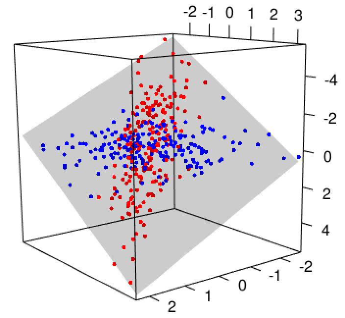
For the shared subspace model, is an anisotropic -dimensional covariance matrix for the projected data, . In contrast, the data projected onto the orthogonal space, , is isotropic for all groups. In Figure 1 we provide a simple illustration using simulated -dimensional data from two groups. In this example, the differences in distribution between the groups of data can be expressed on a two dimensional subspace spanned by the columns of . Differences in the correlations between the two groups manifest themselves on this shared subspace, whereas only the magnitude of the isotropic variability can differ between groups on the orthogonal space. Thus, a shared subspace model can be viewed as a covariance partition model, where one partition includes the anisotropic variability from all groups and the other partition is constrained to the isotropic variability from each group. This isotropic variability is often characterized as measurement noise.
3 Empirical Bayes Inference
In this section we outline an empirical Bayes approach for estimating a low-dimensional shared subspace and the covariance matrices of the data projected onto this space. As we discuss in Section 4, if the spiked covariance model holds for each group individually, then the shared subspace assumption also holds, where the shared subspace is simply the span of the group-specific eigenvectors, . In practice, we can usually identify a shared subspace of dimension that preserves most of the variation in the data. Our primary objective is to identify the “best” shared subspace of fixed dimension . Note that this subspace accounts for the across-group similarity, and thus can be viewed as a hyperparameter in a hierarchical model. Although a fully Bayesian approach may be preferable in the absence of computational limitations, in this paper we propose computationally tractable empirical Bayes inference. In the empirical Bayes approach, hyperparameters are first estimated via maximum marginal likelihood, often using the expectation-maximization algorithm (Lindstrom and Bates, 1988). In many settings such an approach yields group-level inferences that are close to that which would be obtained if the correct across-groups model were known (see for example Efron and Morris, 1973). In Section 3.1 we describe the expectation-maximization algorithm for estimating the maximum marginal likelihood of the shared subspace, . This approach is computationally tractable for high-dimensional data sets. Given an inferred subspace, we then seek estimators for the covariance matrices of the data projected onto this space. Because seemingly large differences in the point estimates of covariance matrices across groups may not actually reflect statistically significant differences, in Section 3.2 we also describe a Gibbs sampler that can be used to generate estimates of the projected covariance matrices, , and their associated uncertainty. Later, in Section 4 we discuss strategies for inferring an appropriate value for and explore how shared subspace models can be used for exploratory data analysis by visualizing covariance heterogeneity on two or three dimensional subspaces.
3.1 Estimating the Shared Subspace
In this section we describe a maximum marginal likelihood procedure for estimating the shared subspace, , based on the expectation-maximization (EM) algorithm. The full likelihood for the shared subspace model can be written as
| (4) |
where we define . The log-likelihood in (up to an additive constant) is
| (5) |
We maximize the marginal likelihood of with an EM algorithm, where and are considered the “missing” parameters. We assume independent Jeffreys prior distributions for both and . The Jeffreys prior distributions for these quantities correspond to and . From the likelihood it can easily be shown that the conditional posterior for is
which is an inverse-Wishart(, ) distribution. The conditional posterior distribution of is simply
which is an inverse-gamma(, ) distribution. We summarize our approach in Algorithm 1 below.
For the M-step, we use a numerical algorithm for optimization over the Stiefel manifold. The algorithm uses the Cayley transform to preserve the orthogonality constraints in and has computationally complexity that is dominated by the dimension of the shared subspace, not the number of features (Wen and Yin, 2013). Specifically, the optimization routine has time complexity O(), and consequently, our approach is computationally efficient for relatively small values of , even when is large. Run times are typically on the order of minutes for values of as large as 10,000 and moderate values of (e.g. ). See Figure 10 in Appendix B for a plot with typical run times in simulations with a range of values of and .
Initialization and Convergence:
The Stiefel manifold is compact and the marginal likelihood is continuous, so the likelihood is bounded. Thus, the EM algorithm, which increases the likelihood at each iteration, will converge to a stationary point (Wu, 1983). However, maximizing the marginal likelihood of the shared subspace model corresponds to a non-convex optimization problem over the Grassmannian manifold and may converge to a sub-optimal local mode or stationary point. Other work involving optimization on the Grassmannian has found convergence to non-optimal stationary values problematic and emphasized the importance of good (e.g. -consistent) starting values (Cook et al., 2016). Our empirical results on simulated data confirms that randomly initialized starting values converge to sub-optimal stationary values, and so in practice we initialize the algorithm at a carefully chosen starting value based on the eigenvectors of a pooled covariance estimate. We give the details for this initialization strategy below.
First, note that when the shared subspace model holds, the first eigenvectors, from any of the groups can be used to construct a -consistent estimator of . In particular, if is the eigenprojection matrix for the subspace spanned by the first eigenvectors of then it can be shown that converges in distribution to a mean-zero normal (Kollo, 2000). In the large , small setting, such classical asymptotic guarantees give little assurance that the resulting estimators would be reasonable, but they nevertheless suggest useful strategies for identifying starting value for the EM algorithm.
In this work, we choose a subspace initialization strategy based on sample eigenvectors of the data pooled from all groups. Let where is a mean-zero normal with covariance and . Then is a mixture of mean-zero normal distributions with covariance
Clearly, the first eigenvectors of span the shared subspace, . This suggests that we can estimate the shared subspace using the scaled and pooled data, , where has dimension . We use as the initial value for subspace estimation algorithm where are the first eigenvectors of . If we treat as an i.i.d. sample from the mixture distribution , then it is known that is not consistent when both and growing at the same rate. For an arbitrary -vector , the asymptotic bias of is well characterized as a function of the eigenvalues of (Mestre, 2008). If either the eigenvalues of or the total sample size are large, will accurately estimate the shared subspace and likelihood based optimization may not be necessary. However, when either the eigenvalues are small or the sample size is small the likelihood based analysis can significantly improve inference and is a useful starting value for the EM algorithm.
Evaluating Goodness of Fit:
Tests for evaluating whether eigenvectors from multiple groups span a common subspace were explored extensively by Schott (1991). These tests can be useful for assessing whether a shared subspace model is appropriate, but cannot be used to test whether a particular subspace explains variation across groups. These results are also based on classical asymptotics and are thus less accurate when
Our goodness of fit measure is based on the fact that when is a basis for a shared subspace, then for each group, most of the non-isotropic variation in should be preserved when projecting the data onto this space. To characterize the extent to which this is true for different groups, we propose a simple estimator for the proportion of “signal” variance that lies on a given subspace. Specifically, we use the following statistic for the ratio of the sum of the first eigenvalues of to the sum of the first eigenvalues of :
| (6) |
where is the Frobenius norm and is a bias correction where with the positive solution to the quadratic equation
| (7) |
and is the -th eigenvalue of .
Theorem 1.
Assume and is fixed. If , then as .
Proof.
Since is fixed and is growing, the numerator, , is a consistent estimator for the sum of the eigenvalues of . In the denominator, is equivalent to the sum of the first eigenvalues of the sample covariance matrix . Baik and Silverstein (2006) and others have demonstrated that asymptotically as and , is positively biased. Specifically,
| (8) |
Replacing by and assuming equality in 8 yields the quadratic equation 7. The solution, , is an asymptotically (in and ) unbiased estimator of and
| (9) |
As such, when the shared subspace model holds both the numerator and denominator of the goodness of fit statistic converge almost surely to . Therefore . ∎
The goodness of fit statistic will be close to one for all groups when is a shared subspace for the data and typically smaller if not. The metric provides a useful indicator of which groups can be reasonably compared on a given subspace and which groups cannot. In practice, we estimate a shared subspace and the isotropic variances using EM and compute the plug-in estimate . When this statistic is small for some groups, it may suggest that the rank of the inferred subspace needs to be larger to capture the variation in all groups. If is substantially larger than 1 for a particular group, it suggests that the inferred subspace is too similar to the sample principal components from group . We investigate these issues in Section 4, by computing the goodness of fit statistic for inferred subspaces of different dimensions on a single data set. In Section 6, we compute the estimates for subspaces inferred with real biological data.
3.2 Inference for Projected Covariance Matrices
The EM algorithm presented in the previous section yields point estimates for , , and but does not lead to natural uncertainty quantification for these estimates. In this section, we assume that the subspace is fixed and known and demonstrate how we can estimate the posterior distribution for . Note that when the subspace is known, the posterior distribution of is conditionally independent from the other groups, so that we can independently estimate the conditional posterior distributions for each group.
There are many different ways in which we could choose to parameterize . Building on recent interest in the spiked covariance model (Donoho et al., 2013; Paul, 2007) we propose a tractable MCMC algorithm by specifying priors on the eigenvalues and eigenvectors of . By modeling the eigenstructure, we can now view each covariance in terms of the original spiked principal components model. Equation 2, written as a function of , becomes
| (10) |
Here, we allow to be of rank dimensional covariance matrix on the -dimensional subspace. Thus, is an diagonal matrix of eigenvalues, and is the matrix of eigenvectors of . For any individual group, this corresponds to the original spiked PCA model (Equation 3) with . Note that the and are jointly unidentifiable because for any orthonormal matrix . Once we fix a basis for the shared subspace, is identifiable. As such, should only be interpreted relative to the basis , as determined by the EM algorithm described in Section 3.1. Differentiating the ranks and is helpful because it enables us to independently specify a subspace common to all groups and the possibly lower rank features on this space that are specific to individual groups.
Although our model is most useful when the covariance matrices are related across groups, we can also use this formulation to specify models for multiple unrelated spiked covariance models. We explore this in detail in Section 4. In Section 6 we introduce a shared subspace model with additional structure on the eigenvectors and eigenvalues of to facilitate interpretation of covariance heterogeneity on a two-dimensional subspace.
The likelihood for given the sufficient statistic is given in Equation 1. For the spiked PCA formulation, we must rewrite this likelihood in terms of , , and . First note that by the Woodbury matrix identity
| (11) |
where the diagonal matrix , e.g. . Further,
| (12) |
where the second line is due to Sylvester’s determinant theorem. Now, the likelihood of , , and is available from Equation 1 by substituting the appropriate quantities for and and replacing with :
| (13) |
We use conjugate and semi-conjugate prior distributions for the parameters , and to facilitate inference via a Gibbs sampling algorithm. In the absence of specific prior information, invariance considerations suggest the use of priors that lead to equivariant estimators. Below we describe our choices for the prior distributions of each parameter and the resultant conditional posterior distributions. We summarise the Gibbs Sampler in Algorithm 2.
Conditional distribution of :
From Equation 13 it is clear that the inverse-gamma class of prior distributions is conjugate for . We chose a default prior distribution for that is equivariant with respect to scale changes. Specifically, we use the Jeffreys prior distribution, an improper prior with density . Under this prior, straightforward calculations show that the full conditional distribution of is inverse-gamma, where .
Conditional distribution of :
Given the likelihood from Equation 13, it is easy to show that the class of Bingham distributions are conjugate for (Hoff, 2009a; Hoff, 2009b). Again, invariance considerations lead us to use a rotationally invariant uniform probability measure on . Under this uniform prior, the full conditional distribution of has a density proportional to the likelihood
| (14) |
This is a Bingham distribution on (Khatri and Mardia, 1977). A Gibbs sampler to simulate from this distribution is given in Hoff (2009b).
Together, the prior for and leads to conditional (on ) Bayes estimators that are equivariant with respect to scale changes and rotations on the subspace spanned by , so that for all and (assuming an invariant loss function). Interestingly, if were known (which it is not), then for a given invariant loss function the Bayes estimator under this prior minimizes the (frequentist) risk among all equivariant estimators (Eaton, 1989).
Conditional distribution for :
Here we specify the conditional distribution of the diagonal matrix . We consider a uniform(0,1) prior distribution for each element of , or equivalently, an prior distribution for the elements of . The full conditional distribution of an element of is proportional to the likelihood function
| (15) | ||||
| (16) |
where and is column of . It is straightforward to show that the density for is proportional to a gamma() truncated at 1. Thus, we can easily sample from this distribution using inversion sampling. The behavior of the distribution for is straightforward to understand: if , then the function has a maximum at , and decays monotonically to zero as . If then the function is uniquely maximized at . To see why this makes sense, note that the likelihood is maximized when the columns of are equal to the eigenvectors of corresponding to its top eigenvalues (Tipping and Bishop, 1999). At this value of , will then equal one of the top eigenvalues of . In the case that , we expect , the true (scaled) population covariance, and so we expect to be near one of the top eigenvalues of , say . If indeed has spikes, then , , and so the conditional mode of is approximately , the correct value. On the other hand, if we have assumed the existence of a spike when there is none, then , and the Bayes estimate of will be shrunk towards zero, as it should be. We summarise the full Gibbs sampling algorithm below.
4 Simulation Studies
We start with an example demonstrating how a shared subspace model can be used to identify statistically significant differences between covariance matrices on a low dimensional subspace. Here, we simulate groups of data from the shared subspace spiked covariance model with features, a shared subspace dimension of , , and . We fix the first eigenvalue of from each group to and vary . We generate the basis for the shared subspace and the eigenvectors of by sampling uniformly from the Stiefel manifold. First, in Figure 2(a) we demonstrate the importance of the eigen-based initialization strategy proposed in Section 3.1. As an accuracy metric, we study the behavior of which is bounded by zero and one and achieves a maximum of one if and only if corresponds to the true shared subspace. In this high dimensional problem, with random initialization, we typically converge to an estimated subspace that has a similarity between 0.25 and 0.5. With the eigen-based initialization we achieve nearly perfect estimation accuracy ().
Next, we summarize estimates of inferred using Algorithm 2 in terms of its eigendecomposition by computing posterior distributions for the log eigenvalue ratio, , with , and the angle of the first eigenvector on this subspace, , relative to the first column of . In Figure 2(b), we depict the 95% posterior regions for these quantities from a single simulation. Dots correspond to the true log ratios and orientations of , where is the maximum marginal likelihood for . To compute the posterior regions, we iteratively remove posterior samples corresponding to the vertices of the convex hull until only 95% of the original samples remain. Non-overlapping posterior regions provide evidence that differences in the covariances are “statistically significant” between groups. In this example, the ratio of the eigenvalues of the true covariance matrices were (black and red groups), (green and blue groups) and (cyan group). Larger eigenvalue ratios correspond to more correlated contours and a value of implies isotropic covariance. Note that for the smaller eigenvalue ratio of , there is more uncertainty about the orientation of the primary axis. When the ratio is one, as is the case for the cyan colored group, there is no information about the orientation of the primary axis since the contours are spherical. In this simulation, the 95% regions all include the true data generating parameters. As we would hope, we find no evidence of a difference between the blue and green groups, since they have overlapping posterior regions. This means that a 95% posterior region for the difference between the groups (0,0), i.e. the model in which the angles and ratios are the same in both groups.
To demonstrate the overall validity of the shared subspace approach, we compute the frequentist coverage of these 95% Bayesian credible regions for the eigenvalue ratio and primary axis orientation using one thousand simulations. For the two groups with eigenvalue ratio the frequentist coverage was close to nominal at approximately 0.94. For the groups with the coverage was approximately 0.92. We did not evaluate the coverage for the group with (cyan) since this value is on the edge of the parameter space and is not covered by the 95% posterior regions as constructed. The slight under coverage for the other groups is likely due to the fact that we infer using maximum marginal likelihood, and thus ignore the extra variability due to the uncertainty about the shared subspace estimate.
4.1 Rank Selection and Model Misspecification
Naturally, shared subspace inference works well when the model is correctly specified. What happens when the model is not well specified? We explore this question in silico by simulating data from different data generating models and evaluating the efficiency of various covariance estimators. In all of the following simulations we evaluate covariance estimates using Stein’s loss, . Since we compute multi-group estimates, we report the average Stein’s loss . Under Stein’s loss, the Bayes estimator is the inverse of the posterior mean of the precision matrix, which we estimate using MCMC samples.
We start by investigating the behavior of our model when we underestimate the true dimension of the shared subspace. In this simulation, we generate groups of mean-zero normally distributed data with , , and . We fix the eigenvalues of to (. Although the signal variance from each group individually is preserved on a two dimensional subspace, these subspaces are not similar across groups since the eigenvectors from each group are generated uniformly from the Stiefel manifold, .
We use these data to evaluate how well the shared subspace estimator performs when we fit the data using a shared subspace model of dimension . In Figure 3(a) we plot Stein’s risk as a function of , estimating the risk empirically using ten independent simulations per value of . The dashed blue line corresponds to Stein’s risk for covariance matrices estimated independently. Independent covariance estimation is equivalent to shared subspace inference with because this implies . Although the risk is large for small values of , as the shared subspace dimension increases to the dimension of the feature space, that is , the risk for the shared subspace estimator quickly decreases. Importantly, it is always true that rank( so it can equivalently be assumed that the data were generated from a shared subspace model with dimension . As such, even when there is little similarity between the eigenvectors from each group, the shared subspace estimator with will perform well, provided that we can identify a subspace, that is close to . When exactly, shared subspace estimation outperforms independent covariance estimation (3(a), dashed red line).
From this simulation, it is clear that correctly specifying the dimension of the shared subspace is important for efficient covariance estimation. When the dimension of the shared subspace is too small, we accrue higher risk. The goodness of fit statistic, , can be used to identify when a larger shared subspace is warranted. When is too small, will be substantially smaller than one for at least some of the groups, regardless of (e.g. Figure 3(b)). When is large enough, we are able to use maximum marginal likelihood to identify a shared subspace which preserves most of the variation in the data for all groups (Figure 3(c)). Thus, for any estimated subspace, the goodness of fit statistic can be used to identify the groups that can be fairly compared on this subspace and whether we would benefit from fitting a model with a larger value of .
Finally, in the appendix, we include a some additional misspecification results. In particular, we consider two cases in a 10 group analysis: one case in which 7 groups share a common subspace but the other three do not, and a second case in which five groups share one common two dimensional subspace, and the other five groups share a different two dimensional subspace (see Figures 8 and 9). Briefly, these results indicate that when only some of the groups share a common subspace, we can still usually identify both the existence of the subspace(s) shared by those groups. We can also identify which groups do not share the space, using the goodness of fit metric. When there are multiple relevant shared subspaces, we can often identify those distinct modes using a different subspace initialization for the EM algorithm.
Model Comparison and Rank Estimation:
Clearly, correct specification for the rank of the shared subspace is important for efficient inference. So far in this section, we have assumed that the group rank, , and shared subspace dimension, , are fixed and known. In practice this is not the case. Prior to fitting a model we should estimate these quantities. Standard model selection methods can be applied to select the both and . Common approaches include cross validation and information criteria like AIC and BIC. However, these approaches are computationally intensive since they require fitting the model for each value of and . Here, we estimate the model dimensions by applying an asymptotically optimal (in mean squared error) singular value threshold for low rank matrix recovery with noisy data (Gavish and Donoho, 2014). This rank estimator is a function of the median singular value of the data matrix and the ratio . Note that under the shared subspace model, the scaled and pooled data described in section 3.1 can be expressed as where are the left singular values of and is a noise matrix with zero mean and variance one. This is the setting in which Gavish and Donoho (2014) develop a rank estimation algorithm, and so it can be appropriately applied to to estimate .
Using this rank estimation approach, we conduct a simulation which demonstrates the relative performance of shared subspace group covariance estimation under different data generating models. We consider three different shared subspace data models: 1) a low dimensional shared subspace model with ; 2) a model in which the spiked covariance matrices from all groups are identical, e.g. ; and 3) a full rank shared subspace model with .
We estimate group-level covariance matrices from simulated data using three different variants of the shared subspace model. For each of these fits we estimate . First, we estimate a single spiked covariance matrix from the pooled data and let . Second, we fit the full rank shared subspace model. This corresponds to a procedure in which we estimate each spiked covariance matrix independently, since implies . Finally, we use an “adaptive” shared subspace estimator, in which we estimate both , and .
Since full rank estimators do not scale well, we compare the performance of various estimators on a simulated data set with only features. We also assume for spikes, , and . We fix the non-zero eigenvalues of to . We simulate 100 independent data sets for each data generating mechanisms. In Table 1 we report the average Stein’s risk and corresponding 95% loss intervals for the estimates derived from each of these inferential models.
| Inferential Model | ||||
|---|---|---|---|---|
| Adaptive | ||||
| Data Model | 0.8 (0.7, 0.9) | 2.1 (1.7, 2.6) | 3.0 (2.9, 3.2) | |
| , | 0.8 (0.7, 0.9) | 0.7 (0.6, 0.8) | 3.0 (2.9, 3.2) | |
| 7.1 (6.2, 8.0) | 138.2 (119, 153) | 3.0 (2.9, 3.2) | ||
As expected, the estimates with the lowest risk are derived from the inferential model that most closely match the data generating specifications. However, the adaptive estimator has small risk under model misspecification relative to the alternatives. For example, when , the adaptive shared subspace estimator has almost four times smaller risk than the full rank estimator, in which each covariance matrix is estimated independently. When the data come from a model in which , that is, the eigenvectors of are generated uniformly from , the adaptive estimator is over an order of magnitude better than the estimator which assumes no differences between groups. These results suggest that empirical Bayes inference for combined with the rank estimation procedure suggested by Gavish and Donoho (2014) can be widely applied to group covariance estimation because the estimator adapts to the amount of similarity across groups. Thus, shared subspace estimation can be an appropriate and computationally efficient choice when the similarity between groups is not known a priori.
Finally, in addition to potential statistical efficiency gains, the empirical Bayes shared subspace estimator has significant computational advantages. In particular, the total run time for empirical Bayes inference of the shared subspace is significantly smaller than full Bayesian inference for a dimensional subspace (e.g. Bayesian probabilistic PCA with ), in particular for larger values of . Given the difficulty of Bayesian inference on the Stiefel manifold, for large , probabilistic principal component analysis quickly becomes infeasible. Empirical Bayes inference enables efficient optimization for and Bayesian inference on the lower dimensional shared subspace (See Figure 10, Appendix B, for typical run times).
5 Reduction of Asymptotic Bias Via Pooling
Recently, there has been an interest in the asymptotic behavior of PCA-based covariance estimators in the setting in which with fixed. Specifically, in the spiked covariance model it is known that when and are both large, the leading eigenvalues of the sample covariance matrix are positively biased and the empirical eigenvectors form a non-zero angle with the true eigenvectors (Baik and Silverstein, 2006; Paul, 2007). Although this fact also implies that the shared subspace estimators are biased, a major advantage of shared subspace inference over independent estimation of multiple covariance matrices is that we reduce the asymptotic bias, relative to independently estimated covariance matrices, by pooling information across groups. The bias reduction appears to be especially large when there is significant heterogeneity in the first eigenvectors of the projected covariance matrices.
Throughout this section we assume groups of data each with observations per group and a fixed constant. First, note that if corresponds to the true shared subspace, then estimates derived using the methods presented in Section 3.2 will consistently estimate as regardless of whether increases as well because has a fixed number of columns. For this reason, we focus explicitly on the accuracy of (derived using the maximum marginal likelihood algorithm presented in Section 3.1) as a function of the number of groups when both and are of the same order of magnitude and much larger than . As an accuracy metric, we again study the behavior of which is bounded by zero and one and achieves a maximum of one if and only if corresponds to the true shared subspace.
Conjecture 1.
Assume that the first eigenvalues from each of groups are identical with . Then, for and , with
| (17) |
We prove that the lower bound in 17 is in fact achieved when are identically distributed and show in simulation that the subspace accuracy exceeds this bound when there is variation in the eigenvectors across groups. In the case of i.i.d. groups, let the covariance matrix have the shared-subspace form given in Equation 2 and without loss of generality let be a diagonal matrix (e.g assume the columns of align with the eigenvectors of ). In this case, the complete data likelihood of (Equation 5) can be rewritten as
where . Since is diagonal and , is diagonal and thus is also diagonal with entries of decreasing magnitude.
Then, the solution to
has equal to the first eigenvectors of . This is maximized when the columns of match the first empirical eigenvectors of and has a maximum of where is the th eigenvalue of . Using a result from Paul (2007), it can be shown that as long as where is the th eigenvalue of , the asymptotic inner product between the th sample eigenvector and the th population eigenvector approaches a limit that is almost surely less than one
As such, we can express asymptotic shared subspace accuracy for the identical groups model as
| (18) |
Here, the accuracy of the estimate depends on , and the magnitude of the eigenvalues, with the bias naturally decreasing as the number of groups increases. Most importantly, Equation 18 provides a useful benchmark for understanding the bias of shared subspace estimates in the general setting in which varies across groups. Our conjecture that the subspace accuracy is larger than the lower bound when the eigenvectors between groups are variable is consistent with our simulation results.
In Figure 4 we depict the subspace accuracy metric and benchmark
for simulated multi-group data generated under the shared subspace model with , , and three different sets of eigenvalues. For each covariance matrix, the eigenvectors of were sampled uniformly from Stiefel manifold . When is isotropic (green) the subspace similarity metric closely matches the benchmark since the assumptions used to derive this asymptotic result are met. However, when the eigenvectors of vary significantly across groups and , the subspace accuracy can far exceed this benchmark (blue). Intuitively, when the first eigenvectors of two different groups are nearly orthogonal, each group provides a lot of information about orthogonal directions on and so the gains in accuracy exceed those that you would get by estimating the subspace from a single group with times the sample size. In general the accuracy of shared subspace estimates depends on the variation in the eigenvectors of across groups as well as the magnitude of the eigenvalues and matrix dimensions and . Although the shared subspace estimator improves on the accuracy of individually estimated covariance matrices, estimates can still be biased when is very large or the eigenvalues of are very small for all . In practice, one should estimate the approximate magnitude of the bias using the inferred eigenvalues of . When these inferred eigenvalues are significantly larger than the bias will likely be small.
6 Analysis of Gene Expression Data
We demonstrate the utility of the shared subspace covariance estimator for exploring differences in the covariability of gene expression levels in young adults with different subtypes of pediatric acute lymphoblastic leukemia (ALL) (Yeoh et al., 2002). Quantifying biological variation across different subtypes of leukemia is important for assigning patients to risk groups, proposing appropriate treatments, and developing a deeper understanding of the mechanisms underlying these different types of cancer. The majority of studies have focused on mean level differences between expression levels. In particular, mean-level differences can be useful for identifying leukemia subtypes. However, differences in the covariance structure across groups can be induced by interactions between important unobserved variables. Covariance analysis is particularly important when the effects of unobserved variables, like disease severity, disease progression or unmeasured genetic confounders, dominate mean level differences across groups. In this analysis, we explicitly remove the mean from the data and look for differences in the covariance structure of the gene expression levels.
The data we analyze were generated from 327 bone marrow samples analyzed on an Affymetrix oligonucleotide microarray with over 12,000 probe sets. Preliminary analysis using mean differences identified clusters corresponding to distinct leukemia subtypes: BCR-ABL, E2A-PBX1, hyperdiploid, MLL, T-ALL, TEL-AML1. 79 patients were assigned to a seventh group for unidentified subtypes (“Others”). We use these labels to stratify the observations into seven groups with corresponding sample sizes of .
Although there are over 12,000 probes on the microarray, the vast majority of gene expression levels are missing. Thus, we restrict our attention to the genes for which less than half of the values are missing and use Amelia, a software package for missing value imputation, to fill in the remaining missing values (Honaker et al., 2011). Amelia assumes the data is missing at random and that each group is normally distributed with a common covariance matrix. Since imputation is done under the assumption of covariance homogeneity, any inferred differences between groups are unlikely to be an artifact of the imputation process. We leave it to future work to incorporate missing data imputation into the shared subspace inference algorithm. After removing genes with very high percentages of missing values, genes remain. Prior to analysis, we de-mean both the rows and columns of the gene expression levels in each group.
We apply the rank selection criteria discussed in Section 4.1 and proposed by Gavish and Donoho (2014) to the pooled expression data (i.e. data from all groups combined) to decide on an appropriate value for the shared subspace. This procedure yields dimensions11 1 Note that for some groups, , in which case we infer the rank matrix .. We run Algorithm 1 to estimate the shared subspace, and then use Bayesian inference (Algorithm 2) to identify differences between groups on the inferred subspace. Together, the run time for the full empirical Bayes procedure (both algorithms) took less than 10 minutes on a 2017 Macbook Pro.
Using the goodness of fit metric, we find that a 45-dimensional shared subspace dimension that explains over of the estimated variation in the top eigenvectors of , suggesting that the rank selection procedure worked reasonably well (Figure 11(a), Appendix B). To further validate the utility of shared subspace modeling, we look at how informative the projected data covariance matrices are for predicting group membership. For an observation , we compute the probability, assuming uniform prior distribution over group membership, that came from group as . We correctly identified the leukemia type in all samples, which provides further confirmation that this subspace provides enough predictive power to easily distinguish groups.
In addition, we quantified differences amongst the projected data covariances using the Frobenius norm, for all pairs of the seven groups. We use these distances to compute a hierarchical clustering dendrogram of the groups (Figure 11(b), Appendix B). The hierarchical clustering reveals that BCR-ABL, E2A-PBX1, TEL-AML1 and hyperdiploid, which correspond to B lineage leukemias, cluster together. T-ALL, the T lineage leukemia, and MLL, the mixed lineage leukemia, appear the most different (Dang, 2012). To further verify that the inferred subspace relates to relevant biological processes, we conducted gene set enrichment analysis using the observed magnitudes of the loadings for the genes on the 45 basis vectors (Subramanian et al., 2005) and using gene sets defined by the Gene Ontology Consortium (Consortium et al., 2004). Gene set analysis on the magnitudes of gene loadings identified dozens of pathways (FDR , (Storey et al., 2003)). Nearly every identified pathway relates to the immune response or cell growth (Figure 12, Appendix B), for example B and T cell proliferation (GO:0042100, GO:0042102), immunoglobin receptor binding (GO:0034987) and cellular response to cytokine stimulus (GO:0071345) to name only a few. Together, all of these results suggest that in this application there is indeed significant differences in the covariability between genes for each the of groups, with biologically plausible underpinnings. Consequently, there is value in exploring what underlies those differences.
We next demonstrate how we can explore significant a posteriori differences between the groups which might lead to scientifically meaningful insights. In order to visualize differences in the posterior distributions of the dimensional matrices , we examine the distribution of eigenvalues and eigenvectors between the groups on a variety of two-dimensional subspaces of the shared space. We propose two different methods for identifying potentially interesting sub-subspaces to visualize. First, we summarize variation on a two dimensional subspace whose axes are approximately aligned to the first two eigenvectors of , for a specific group . This subspace corresponds to the subspace of maximal variability within group . For example, in Figure 5(a) we plot posterior summaries about the principal eigenvector and eigenvalues for each group on a two dimensional space spanned by the first two eigenvectors of the inferred covariance matrix for the hyperdiploid group. The -axis corresponds to the orientation of the first eigenvector and the y-axis corresponds the magnitude of the first eigenvalue. In this subspace, we can see that the first eigenvector for most groups appear to have similar orientations, but that the hyperdiploid group has significantly larger variance along the first principal component direction than all other groups (with the exception of perhaps T-ALL, for which the posterior samples overlap). The first eigenvector for the BCR-ABL subgroup appears to be the least variable on this subspace.
As an alternative approach to summarizing the posterior distribution, we examine the posterior eigen-summaries on a two dimensional subspace which is chosen to maximize the difference between any two chosen groups. To achieve this, we look at spaces in which the axes correspond to the first two eigenvectors of for any . As an example, in Figure 5(b) we plot posterior summaries corresponding to the subspace for which the difference between the T-ALL and MLL subgroups is large. On this subspace, the groups cluster into four distinct subgroups which appear significantly different a posteriori: the T-ALL subtype, the MLL subtype, the BCR subtype and the all other groups. Roughly, along the first dimension, there is large variability in the T-ALL group that is not matched in other groups, whereas the second dimension there is large variability in the MLL group that is not matched in the other groups.
Scientific insights underlying the significant differences that were identified in Figure 5 can be understood in the biplots in Figures 6 and 7. In each figure, we plot the contours of the two dimensional covariance matrices for a few leukemia subtypes. The 20 genes with the largest loadings for one of the component directions are indicated with letters and the remaining loadings plotted with light grey dots. The gene names for the genes with the largest loadings are listed in the corresponding table. In both biplots, the identified genes have known connections to cancer, leukemia, and the immune system.
For example, for the subspace of maximal variability in the hyperdiploid group, gene set analysis identified two gene sets with large magnitude loadings on the first principal component: a small group of proteins corresponding to the MHC class II protein complex (GO:0006955) as well as a larger group of genes corresponding to genes generally involved in immune response (GO:0006955). MHC class II proteins are known to play an essential role in the adaptive immune system (Reith et al., 2005) and are correlated with leukemia patient outcomes (Rimsza et al., 2004). Our analysis indicates these proteins have especially variable levels in the hyperdiploid subtype relative to the other leukemia subtypes.
Positive Negative A HLA-DQB1 K BCL11A B HBG1 L HHLA1 C SASH3 M D HLA-DPB1 N CSHL1 E MME O NF2 F HLA-DQB1 P SKAP2 G DPYSL2 Q TRDV2 H PRPF6 R EIF2AK2 I ADA S J ATP6V0E2 T PMF1
Positive Negative A SELL K AHNAK B CD24 L NR3C1 C SH3BP5 M LMO2 D LEF1 N NR3C1 E CCR7 O GSN F WASF1 P SERPINB1 G LSP1 Q CSHL1 H FADS3 R DPYSL2 I LCK S NKG7 J LCK T DAD1
For the subspace chosen to maximize the difference between T-ALL and MLL groups, gene set analysis associated with large loadings in the second dimension (associated with high variance in the MLL subgroup) included “regulation of myeloid cell differentiation” (GO:0045637), “positive regulation of B cell receptor signaling pathway” (GO:0098609) and “immunoglobulin V(D)J recombination” (GO:0033152). Most of the individual genes with large loadings are known in the leukemia literature including WASF1 (“F”) which plays an important role in apoptosis (Kang et al., 2010), LEF1 (“D”) which is linked to the pathogenesis of leukemia (Gutierrez et al., 2010) and LMO2 (“M”) which was shown to initiate leukemia in mice (McCormack et al., 2010), to name only a few. In contrast to the MLL group, these genes in the T-ALL and TEL-AML1 subgroups have relatively little variability.
These insights would be overlooked in more conventional mean-based analyses, particularly when mean-level differences are small relative to the residual variance. Further, we have shown how the shared subspace reveals sets of interpretable genes that are most important for describing difference between leukemia subtypes; these discoveries would less evident with alternative covariance estimation methods which do not explicitly include the assumption about differences manifesting on a common low dimensional subspace. All told, these results highlight the value of shared subspace covariance matrix inference for both predicting leukemia subtypes as well as for exploring scientifically meaningful differences between the groups.
7 Discussion
In this paper, we proposed a class of models for estimating and comparing differences in covariance matrices across multiple groups on a common low dimensional subspace. We described an empirical Bayes algorithm for estimating this common subspace and a Gibbs sampler for inferring the projected covariance matrices and their associated uncertainty. Estimates of both the shared subspace and the projected covariance matrices can both be useful summaries of the data. For example, with the leukemia data, the shared subspace highlights the full set of genes that are correlated across groups. Differences between group covariance matrices can be understood in terms of differences in these sets of correlated molecules. In this analysis, we demonstrated how we can use these notions to visualize and contrast the posterior distributions of covariance matrices projected onto a particular subspace and interpret these differences biologically.
In simulation, we showed that the shared subspace model can still be a reasonable choice for modeling multi-group covariance matrices even when the groups may be largely dissimilar. When there is little similarity between groups, the shared subspace model can still be appropriate as long as the dimension of the shared subspace is large enough. However, selecting the rank of the shared subspace remains a practical challenge. Although we propose a useful heuristic for choosing the dimension of the shared subspace based on the rank selection estimators of Gavish and Donoho (2014), a more principled approach is warranted. Improved rank estimators would further improve the performance of the adaptive shared subspace estimator discussed in Section 4.
It is also a challenging problem to estimate the “best” subspace once the rank of the space is specified. We used maximum marginal likelihood to estimate and then used MCMC to infer . By focusing on group differences for on a fixed subspace, it is much simpler to interpret similarities and differences. Nevertheless, full uncertainty quantification for can be desirable. We found MCMC inference for to be challenging for the problems considered in this paper and leave it for future work to develop an efficient fully Bayesian approach for estimating the joint posterior of and . Recently developed Markov chain Monte Carlo algorithms, like Riemannian manifold Hamilton Monte Carlo, which can exploit the geometry of the Grassmannian manifold, may be useful here (Byrne and Girolami, 2013; Girolami and Calderhead, 2011). It may also be possible, though computationally intensive, to jointly estimate and using for instance, a reversible-jump MCMC algorithm.
Fundamentally, our approach is quite general and can be integrated with existing approaches for multi-group covariance estimation. In particular, we can incorporate additional shrinkage on the projected covariance matrices . As in Hoff (2009a) we can employ non-uniform Bingham prior distributions for the eigenvectors of or we can model as a function of continuous covariates as in Yin et al. (2010) and Hoff and Niu (2012). Alternatively, we can summarize the estimated covariance matrices by thresholding entries of the precision matrix, to visualize differences between groups using a graphical model (Meinshausen and Bühlmann, 2006). We can also incorporate sparsity to the estimated eigenvectors of the shared subspace to add in interpretation (Ročková and George, 2016, e.g). Finally, we can consider variants in which some eigenvectors are assumed to be identical across groups, whereas others are allowed to vary on the shared subspace. This can further improve estimation efficiency, particularly when the common eigenvectors are associated with the largest eigenvalues and differences appear in lower variance components (Cook and Forzani, 2008). Such an approach would further aid in identifying the relevant sub-subspace of variability that describes prominent differences between groups . The specifics of the problem at hand should dictate which extensions are appropriate, but the shared subspace assumption can be useful in a wide range of analyses, especially when the number of features is very large. A repository for the replication code is available on GitHub (Franks, 2016).
Appendix A Additional Misspecification Results
Following the simulation set up of 4.1 we generate data from 10 groups with , and . In this section, we consider two model misspecification simulations. First, we consider data in which the first two eigenvectors for the first five groups share a two-dimensional subspace, and the eigenvectors for the last five groups share a different two-dimensional subspace. We then fit all ten groups assuming a two-dimensional shared subspace model. In Figure 8 we plot the goodness of fit metric for all ten groups for subspaces identified in different local modes of the likelihood. Specifically, we empirically identified three local modes: one mode identifies the shared subspace for the first give groups, the other mode corresponds to the shared subspace for the second five groups, and the third mode corresponds to subspace shares some commonalities across all 10 groups. This last mode is the one discovered by the eigen-based initialization strategy proposed in Section 4.1.
In the second simulation we generate the first two eigenvectors for the first seven groups from a common two dimensional subspace. The eigenvectors from the last three groups were generated uniformly at random from the dimensional null space of the shared subspace. In repeated simulations with initialized uniformly at random on the Stiefel manifold, the resulting we empirically discovered four modes. In Figure 9 we plot goodness of fit metrics for the 10 groups at these modes. The first mode corresponds to the shared subspace for the first 7 groups. The other three modes identify subspaces shared by two of the last three groups.
Appendix B Run time results
Appendix C Addition Results From Leukemia Analysis
Name Q-value Number of Genes GO:0005751 mitochondrial respiratory chain complex IV 0.00 7 GO:0044388 small protein activating enzyme binding 0.01 7 GO:0022624 proteasome accessory complex 0.00 16 GO:0048025 negative regulation of nuclear mRNA splicing, via spliceosom 0.01 21 GO:0004298 threonine-type endopeptidase activity 0.01 19 GO:0010498 proteasomal protein catabolic process 0.01 26 GO:0006405 RNA export from nucleus 0.00 33 GO:0031124 mRNA 3’-end processing 0.00 36 GO:0030336 negative regulation of cell migration 0.01 22 GO:0038083 peptidyl-tyrosine autophosphorylation 0.01 20 GO:0043235 receptor complex 0.00 18 GO:0045766 positive regulation of angiogenesis 0.00 36 GO:0048661 positive regulation of smooth muscle cell proliferation 0.00 18 GO:0035690 cellular response to drug 0.00 27 GO:0060337 type I interferon-mediated signaling pathway 0.00 32 GO:0000786 nucleosome 0.00 27 GO:0004888 transmembrane signaling receptor activity 0.00 27 GO:0030183 B cell differentiation 0.00 30 GO:0030890 positive regulation of B cell proliferation 0.01 15 GO:0060333 interferon-gamma-mediated signaling pathway 0.00 35 GO:0030198 extracellular matrix organization 0.00 23 GO:0002053 positive regulation of mesenchymal cell proliferation 0.01 9 GO:0071345 cellular response to cytokine stimulus 0.01 19 GO:0007159 leukocyte cell-cell adhesion 0.00 16 GO:0034113 heterotypic cell-cell adhesion 0.00 10 GO:0042102 positive regulation of T cell proliferation 0.00 19 GO:0042605 peptide antigen binding 0.00 15 GO:0030658 transport vesicle membrane 0.00 13 GO:0071556 integral to lumenal side of endoplasmic reticulum membrane 0.01 17 GO:0042613 MHC class II protein complex 0.00 10 GO:0004896 cytokine receptor activity 0.00 9 GO:0005001 transmembrane receptor protein tyrosine phosphatase activity 0.01 7 GO:0030669 clathrin-coated endocytic vesicle membrane 0.00 10 GO:0042100 B cell proliferation 0.00 14 GO:0042742 defense response to bacterium 0.00 35 GO:0031668 cellular response to extracellular stimulus 0.00 13 GO:0001916 positive regulation of T cell mediated cytotoxicity 0.01 10 GO:0019731 antibacterial humoral response 0.00 19 GO:0001915 negative regulation of T cell mediated cytotoxicity 0.00 6 GO:0072562 blood microparticle 0.00 32 GO:0035456 response to interferon-beta 0.01 7 GO:0050829 defense response to Gram-negative bacterium 0.00 13 GO:0003823 antigen binding 0.00 24 GO:0071757 hexameric IgM immunoglobulin complex 0.00 6 GO:0006911 phagocytosis, engulfment 0.00 23 GO:0042834 peptidoglycan binding 0.00 7 GO:0071756 pentameric IgM immunoglobulin complex 0.00 7 GO:0006958 complement activation, classical pathway 0.00 19 GO:0006910 phagocytosis, recognition 0.00 16 GO:0042571 immunoglobulin complex, circulating 0.00 16 GO:0050871 positive regulation of B cell activation 0.00 16 GO:0003094 glomerular filtration 0.00 7 GO:0034987 immunoglobulin receptor binding 0.00 17 GO:0001895 retina homeostasis 0.00 11
References
- Baik and Silverstein [2006] Jinho Baik and Jack W. Silverstein. Eigenvalues of large sample covariance matrices of spiked population models. Journal of Multivariate Analysis, 97(6):1382–1408, 2006. ISSN 0047259X. doi: 10.1016/j.jmva.2005.08.003. URL http://linkinghub.elsevier.com/retrieve/pii/S0047259X0500134X.
- Barker and Rayens [2003] Matthew Barker and William Rayens. Partial least squares for discrimination. Journal of Chemometrics, 17(3):166–173, 2003. ISSN 08869383. doi: 10.1002/cem.785. URL http://dx.doi.org/10.1002/cem.785.
- Bellet et al. [2012] Aurélien Bellet, Amaury Habrard, and Marc Sebban. Similarity learning for provably accurate sparse linear classification. arXiv preprint arXiv:1206.6476, 2012.
- Boik [2002] Robert J Boik. Spectral models for covariance matrices. Biometrika, 89(1):159–182, 2002.
- Byrne and Girolami [2013] Simon Byrne and Mark Girolami. Geodesic Monte Carlo on embedded manifolds. Scandinavian Journal of Statistics, 40(4):825–845, 2013.
- Chikuse [2012] Yasuko Chikuse. Statistics on special manifolds, volume 174. Springer Science & Business Media, 2012.
- Consortium et al. [2004] Gene Ontology Consortium et al. The gene ontology (go) database and informatics resource. Nucleic acids research, 32(suppl 1):D258–D261, 2004.
- Cook [2009] R Dennis Cook. Regression graphics: ideas for studying regressions through graphics, volume 482. John Wiley & Sons, 2009.
- Cook and Forzani [2008] R Dennis Cook and Liliana Forzani. Covariance reducing models: An alternative to spectral modelling of covariance matrices. Biometrika, 95(4):799–812, 2008.
- Cook et al. [2016] R. Dennis Cook, Liliana Forzani, and Zhihua Su. A note on fast envelope estimation. Journal of Multivariate Analysis, 150:42–54, 2016. ISSN 10957243. doi: 10.1016/j.jmva.2016.05.006. URL http://dx.doi.org/10.1016/j.jmva.2016.05.006.
- Danaher et al. [2014] Patrick Danaher, Pei Wang, and Daniela M. Witten. The joint graphical lasso for inverse covariance estimation across multiple classes. Journal of the Royal Statistical Society. Series B: Statistical Methodology, 76(2):373–397, 2014. ISSN 13697412. doi: 10.1111/rssb.12033.
- Dang [2012] Chi V Dang. Myc on the path to cancer. Cell, 149(1):22–35, 2012.
- Donoho et al. [2013] David L Donoho, Matan Gavish, and Iain M Johnstone. Optimal shrinkage of eigenvalues in the spiked covariance model. arXiv preprint arXiv:1311.0851, 2013.
- Eaton [1989] Morris L Eaton. Group invariance applications in statistics. In Regional conference series in Probability and Statistics, pages i–133. JSTOR, 1989.
- Efron and Morris [1973] Bradley Efron and Carl Morris. Stein’s estimation rule and its competitors—an empirical bayes approach. Journal of the American Statistical Association, 68(341):117–130, 1973.
- Flury [1987] BK Flury. Two generalizations of the common principal component model. Biometrika, 74(1):59–69, 1987. ISSN 00063444. doi: 10.2307/2336021. URL http://biomet.oxfordjournals.org/content/74/1/59.short.
- Franks [2016] Alexander M. Franks. Replication code for shared subspace estimation. https://github.com/afranks86/shared-subspace, 2016.
- Gavish and Donoho [2014] Matan Gavish and David L Donoho. The optimal hard threshold for singular values is . Information Theory, IEEE Transactions on, 60(8):5040–5053, 2014.
- Girolami and Calderhead [2011] Mark Girolami and Ben Calderhead. Riemann manifold Langevin and Hamiltonian Monte Carlo methods. Journal of the Royal Statistical Society. Series B: Statistical Methodology, 73:123–214, 2011. ISSN 13697412. doi: 10.1111/j.1467-9868.2010.00765.x.
- Gutierrez et al. [2010] Alejandro Gutierrez, Takaomi Sanda, Wenxue Ma, Jianhua Zhang, Ruta Grebliunaite, Suzanne Dahlberg, Donna Neuberg, Alexei Protopopov, Stuart S Winter, Richard S Larson, et al. Inactivation of lef1 in t-cell acute lymphoblastic leukemia. Blood, 115(14):2845–2851, 2010.
- Heimberg et al. [2016] Graham Heimberg, Rajat Bhatnagar, Hana El-Samad, and Matt Thomson. Low dimensionality in gene expression data enables the accurate extraction of transcriptional programs from shallow sequencing. Cell Systems, 2(4):239–250, 2016.
- Hoff [2009a] Peter D Hoff. A hierarchical eigenmodel for pooled covariance estimation. Journal of the Royal Statistical Society: Series B (Statistical Methodology), 71(5):971–992, 2009a.
- Hoff [2009b] Peter D Hoff. Simulation of the matrix Bingham–von Mises–Fisher distribution, with applications to multivariate and relational data. Journal of Computational and Graphical Statistics, 2009b.
- Hoff and Niu [2012] Peter D Hoff and Xiaoyue Niu. A covariance regression model. Statistica Sinica, 22:729–753, 2012.
- Honaker et al. [2011] James Honaker, Gary King, and Matthew Blackwell. Amelia II: A program for missing data. Journal of Statistical Software, 45(7):1–47, 2011. URL http://www.jstatsoft.org/v45/i07/.
- Huang and Van Gool [2017] Zhiwu Huang and Luc Van Gool. A riemannian network for spd matrix learning. In Thirty-First AAAI Conference on Artificial Intelligence, 2017.
- Johnstone [2001] Iain M Johnstone. On the distribution of the largest eigenvalue in principal components analysis. Annals of statistics, pages 295–327, 2001.
- Kanamori and Takeda [2012] Takafumi Kanamori and Akiko Takeda. Non-convex optimization on stiefel manifold and applications to machine learning. In International Conference on Neural Information Processing, pages 109–116. Springer, 2012.
- Kang et al. [2010] R Kang, D Tang, Y Yu, Z Wang, T Hu, H Wang, and L Cao. Wave1 regulates bcl-2 localization and phosphorylation in leukemia cells. Leukemia, 24(1):177, 2010.
- Khatri and Mardia [1977] CG Khatri and KV Mardia. The von Mises-Fisher matrix distribution in orientation statistics. Journal of the Royal Statistical Society. Series B (Methodological), pages 95–106, 1977.
- Kiefer and Schwartz [1965] J Kiefer and R Schwartz. Admissible Bayes character of T2-, R2-, and other fully invariant tests for classical multivariate normal problems. The Annals of Mathematical Statistics, pages 747–770, 1965.
- Kollo [2000] Tõnu Kollo. Asymptotic inference based on eigenprojections of covariance and correlation matrices. In Innovations in Multivariate Statistical Analysis, pages 207–222. Springer, 2000.
- Lindstrom and Bates [1988] Mary J Lindstrom and Douglas M Bates. Newton—raphson and em algorithms for linear mixed-effects models for repeated-measures data. Journal of the American Statistical Association, 83(404):1014–1022, 1988.
- Liu et al. [2009] Jun Liu, Shuiwang Ji, and Jieping Ye. Multi-task feature learning via efficient l 2, 1-norm minimization. In Proceedings of the twenty-fifth conference on uncertainty in artificial intelligence, pages 339–348. AUAI Press, 2009.
- Mardia et al. [1980] Kantilal Varichand Mardia, John T Kent, and John M Bibby. Multivariate analysis. Academic press, 1980.
- McCormack et al. [2010] Matthew P McCormack, Lauren F Young, Sumitha Vasudevan, Carolyn A de Graaf, Rosalind Codrington, Terence H Rabbitts, Stephen M Jane, and David J Curtis. The lmo2 oncogene initiates leukemia in mice by inducing thymocyte self-renewal. Science, 327(5967):879–883, 2010.
- Meinshausen and Bühlmann [2006] Nicolai Meinshausen and Peter Bühlmann. High-dimensional graphs and variable selection with the lasso. The annals of statistics, pages 1436–1462, 2006.
- Mestre [2008] Xavier Mestre. On the asymptotic behavior of the sample estimates of eigenvalues and eigenvectors of covariance matrices. IEEE Transactions on Signal Processing, 56(11):5353–5368, 2008.
- Paul [2007] Debashis Paul. Asymptotics of sample eigenstructure for a large dimensional spiked covariance model. Statistica Sinica, pages 1617–1642, 2007.
- Pham and Venkatesh [2008] Duc-Son Pham and Svetha Venkatesh. Robust learning of discriminative projection for multicategory classification on the stiefel manifold. In 2008 IEEE Conference on Computer Vision and Pattern Recognition, pages 1–7. IEEE, 2008.
- Reith et al. [2005] Walter Reith, Salomé LeibundGut-Landmann, and Jean-Marc Waldburger. Regulation of mhc class ii gene expression by the class ii transactivator. Nature Reviews Immunology, 5(10):793, 2005.
- Rimsza et al. [2004] Lisa M Rimsza, Robin A Roberts, Thomas P Miller, Joseph M Unger, Michael LeBlanc, Rita M Braziel, Dennis D Weisenberger, Wing C Chan, H Konrad Muller-Hermelink, Elaine S Jaffe, et al. Loss of mhc class ii gene and protein expression in diffuse large b-cell lymphoma is related to decreased tumor immunosurveillance and poor patient survival regardless of other prognostic factors: a follow-up study from the leukemia and lymphoma molecular profiling project. Blood, 103(11):4251–4258, 2004.
- Ročková and George [2016] Veronika Ročková and Edward I George. Fast bayesian factor analysis via automatic rotations to sparsity. Journal of the American Statistical Association, 111(516):1608–1622, 2016.
- Romero et al. [2016] Daniel Romero, Dyonisius Dony Ariananda, Zhi Tian, and Geert Leus. Compressive covariance sensing: Structure-based compressive sensing beyond sparsity. IEEE signal processing magazine, 33(1):78–93, 2016.
- Schott [1991] James R Schott. Some tests for common principal component subspaces in several groups. Biometrika, 78(4):771–777, 1991.
- Schott [1999] James R Schott. Partial common principal component subspaces. Biometrika, 86(4):899–908, 1999.
- Storey et al. [2003] John D Storey et al. The positive false discovery rate: a bayesian interpretation and the q-value. The Annals of Statistics, 31(6):2013–2035, 2003.
- Subramanian et al. [2005] Aravind Subramanian, Pablo Tamayo, Vamsi K Mootha, Sayan Mukherjee, Benjamin L Ebert, Michael A Gillette, Amanda Paulovich, Scott L Pomeroy, Todd R Golub, Eric S Lander, et al. Gene set enrichment analysis: a knowledge-based approach for interpreting genome-wide expression profiles. Proceedings of the National Academy of Sciences, 102(43):15545–15550, 2005.
- Tipping and Bishop [1999] Michael E Tipping and Christopher M Bishop. Probabilistic principal component analysis. Journal of the Royal Statistical Society: Series B (Statistical Methodology), 61(3):611–622, 1999.
- Vemulapalli et al. [2013] Raviteja Vemulapalli, Jaishanker K Pillai, and Rama Chellappa. Kernel learning for extrinsic classification of manifold features. In Proceedings of the IEEE Conference on Computer Vision and Pattern Recognition, pages 1782–1789, 2013.
- Wang and Sun [2015] Fei Wang and Jimeng Sun. Survey on distance metric learning and dimensionality reduction in data mining. Data Mining and Knowledge Discovery, 29(2):534–564, 2015.
- Wen and Yin [2013] Zaiwen Wen and Wotao Yin. A feasible method for optimization with orthogonality constraints. Mathematical Programming, 142(1-2):397–434, 2013.
- Wold et al. [2001] Svante Wold, Michael Sjöström, and Lennart Eriksson. Pls-regression: a basic tool of chemometrics. Chemometrics and intelligent laboratory systems, 58(2):109–130, 2001.
- Wu [1983] CF Jeff Wu. On the convergence properties of the em algorithm. The Annals of statistics, pages 95–103, 1983.
- Yeoh et al. [2002] Eng-Juh Yeoh, Mary E Ross, Sheila A Shurtleff, W Kent Williams, Divyen Patel, Rami Mahfouz, Fred G Behm, Susana C Raimondi, Mary V Relling, Anami Patel, et al. Classification, subtype discovery, and prediction of outcome in pediatric acute lymphoblastic leukemia by gene expression profiling. Cancer cell, 1(2):133–143, 2002.
- Yin et al. [2010] Jianxin Yin, Zhi Geng, Runze Li, and Hansheng Wang. Nonparametric covariance model. Statistica Sinica, 20:469, 2010.
- Zhang et al. [2016] Xiaotong Zhang, Xianchao Zhang, Han Liu, and Xinyue Liu. Multi-task multi-view clustering. IEEE Transactions on Knowledge and Data Engineering, 28(12):3324–3338, 2016.