Incremental Factorization Machines for Persistently Cold-starting Online Item Recommendation

Vinagre et al. [10] proposed an efficient iMF algorithm for item recommendation, which is achieved by solving MF with a unique target value $y=1$ over the stochastic gradient descent (SGD) optimization. Moreover, they evaluated the method in a test-then-learn scheme as outlined in Alg. 1. For each pair of a user $u\in U$ and an item $i\in I$, evaluation is first launched before updating the parameters.

More specifically, iMF incrementally factorizes a binary matrix $R\in\mathbb{R}^{|U|\times|I|}$ into $P\in\mathbb{R}^{|U|\times k}$ and $Q\in\mathbb{R}^{|I|\times k}$ as:

• •

  Step 1: Learn $P$ and $Q$ as the standard MF

• •

  Step 2: Score items by $Q\ \mathbf{p}_{u}\in\mathbb{R}^{|I|}$, and
  recommend $N$ closest items to $1$

• •

  Step 3: $\mathbf{p}_{u}\leftarrow\mathbf{p}_{u}+2\eta\ \left(\left(1-\mathbf{p}_{u}^{\mathrm{T}}\mathbf{q}_{i}\right)\ \mathbf{q}_{i}-\lambda\ \mathbf{p}_{u}\right)$
  $\mathbf{q}_{i}\leftarrow\mathbf{q}_{i}+2\eta\ \left(\left(1-\mathbf{p}_{u}^{\mathrm{T}}\mathbf{q}_{i}\right)\ \mathbf{p}_{u}-\lambda\ \mathbf{q}_{i}\right)$

where $\mathbf{p}_{u},\mathbf{q}_{i}\in\mathbb{R}^{k}$ are respectively a user, item latent vector. The vectors are updated with a regularization parameter $\lambda$ and a learning rate $\eta$.

FMs [7] have been recently developed as a general predictor. For an input vector $\mathbf{x}\in\mathbb{R}^{d}$, let us first imagine a linear model parameterized by $w_{0}\in\mathbb{R}$，$\mathbf{w}\in\mathbb{R}^{d}$. In addition, by incorporating interactions of the $d$ input variables, the linear model is extended to FMs as:

where $V\in\mathbb{R}^{d\times k}$ is a rank-$k$ matrix which has $\mathbf{v}_{1},\cdots,\mathbf{v}_{d}\in\mathbb{R}^{k}$. Arbitrary feature representation $\mathbf{x}$ (e.g. concatenation of one-hot vectors for several categorical variables) work well with FMs, and MF is actually a subset of the predictor.

This paper focuses on running FMs in an incremental fashion. Generally, learning FM requires a set of parameters $\Theta=\{w_{0},\mathbf{w},V\}$ and a loss function $\ell(\hat{y}(\mathbf{x}\mid\Theta),y)$, and the parameters can be optimized by SGD. Specifically, for a set of samples $S$, the parameters of FM are updated as Alg. 2. For simplicity, $\ell(\hat{y}(\mathbf{x}\mid\Theta),y)$ is written as $\ell$.

Notice that Step 3 of iMF in Sec. 2.1 is SGD update for single sample, so the basic idea of this paper is that we replace the step with $\Theta$-update in Alg. 2. As a result, iFM which can be evaluated in the test-then-learn scheme is derived without loss of generality.

Rendle [8] proposed an adaptive regularization scheme for FMs. As shown in Alg. 3, the technique adjusts the regularization parameters by using a sample $(\mathbf{x}^{\prime},y^{\prime})$ in a validation set $S^{\prime}$, an extra set of samples which is different from $S$.

Normally, Alg. 3 is launched after $\Theta$-update in Alg. 2. However, when we consider incremental adaptive regularization, there is a difficulty that the validation set $S^{\prime}$ will be gradually outdated in a streaming environment. A key idea to conquer the problem is that a newly observed sample $(\mathbf{x},y)$ is handled as a pseudo validation sample, so the regularization parameters are adjusted before updating $\Theta$ as demonstrated in Fig. 2.

This section considers a particular combination of an output $y$ and a loss function $\ell$ to utilize iFMs for online item recommendation. As the author explained in Sec. 2.1, iMF actually solves MF with $y=1$. Similarly to the approach, let us again consider the unique output for a set of positive events $S_{+}$. As a consequence, for a sample $(\mathbf{x},1)\in S_{+}$, our loss function is defined as: $\ell(\hat{y}(\mathbf{x}\mid\Theta),1)=(\hat{y}(\mathbf{x}\mid\Theta)-1)^{2}$.

Eventually, for arbitrary design of a feature vector $\mathbf{x}$, the proposed iFM-based item recommender which is feasible in a streaming environment can be described in the test-then-learn framework as:

• •

  Step 1: Learn $w_{0}$, $\mathbf{w}$ and $V$ as the standard FMs

• •

  Step 2: Predict $\hat{y}(\mathbf{x}\mid\Theta)$ for every items,
  and recommend $N$ closest items to $1$

• •

  Step 3: $\lambda$-update $\rightarrow$ $\Theta$-update with $(\mathbf{x},1)$

Importantly, since the number of users and items on real-world online applications is not constant, our systems must incorporate new users and items into a current model somehow. For example, iMF handles a new user (item) as an additional row of $P$ ($Q$) (i.e. $\mathbf{p}_{|U|+1}$ for a new user, $\mathbf{q}_{|I|+1}$ for a new item obtained from Gaussian). Hence, iFMs also take the simple approach that a zero and random vector are respectively inserted into $\mathbf{w}$ and $V$ as the initial parameters of new features. Fig. 3 depicts detection and insertion of new features in a stream of input vectors. It is notable that, beyond new users and items, adding new contextual variables is also possible in the middle of data streams.

In terms of computational complexity, iFMs compute the interaction term $\sum_{i=1}^{d}\sum_{j=i}^{d}\mathbf{v}_{i}^{\mathrm{T}}\mathbf{v}_{j}x_{i}x_{j}$ in $\mathcal{O}\left(kN_{z}(\mathbf{x})\right)$ by letting the number of nonzero elements in $\mathbf{x}$ be $N_{z}(\mathbf{x})$. In fact, this complexity is efficient enough due to sparsity of $\mathbf{x}$, but running time will be relatively long compared to the single vector updating of iMF. Therefore, there is trade-off between running time and context-awareness in practice.

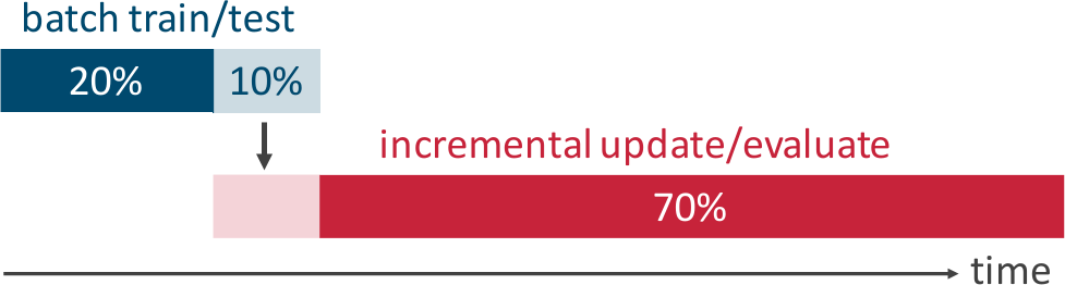
In the experiments, the test-then-learn procedure described in Sec. 2.1 is launched for time-stamped unstable datasets. As shown in Fig. 4, the samples are separated similarly to what Matuszyk et al. [6] did. At the beginning, a batch train/test step is executed for the first 20% training and following 10% validation samples. Next, the 10% samples are just used for one-pass model updating, and the incremental evaluation step is finally performed for the remaining 70%.

Additionally, the 70% samples are also evaluated by mean percentile rank (MPR) in order to assess an ordered list of items obtained from Step 2. The metric is calculated based on percentile rank of the correct items in the ordered lists; that is, $\mathrm{MPR}=0\%$ indicates the best result that a recommender always gives the highest rank to a correct item, and $\mathrm{MPR}=100\%$ is opposite. In contrast to recall@$N$/$T$ which evaluates top-$N$ items, MPR can measure users’ overall satisfaction from all items.

Following methods were employed as the competitors:

• •

  static MF: the traditional MF,

• •

  iMF: a fast extension of MF introduced in Sec. 2.1,

• •

  static FMs: the parameters are not updated in the incremental stage similarly to static MF.

The author implemented all of the methods in Python 3.5.1, and the code was run in a typical personal computer with the 2.7 GHz Intel® Core™ i7 CPU and 4GB RAM.

Datasets used in the experiments were binarized version of MovieLens 100k (ML100k)¹¹ 1 http://grouplens.org/datasets/movielens/ and synthetic click data; the former is a real-world example of user-side volatility, and the latter shows item-side instability. Table 1 summarizes statistics of the data. Each pair of a method and a dataset was tested five times with different initial parameters.

Most users on ML100k report positive events just for the initial rating activity, and they do not rate any more. Even if some users continuously rate movies, intuition tells us that their interests change over time. Thus, ML100k is a real-world example of user-side persistent cold-start.

Fig. 5 shows the best recall behaviors on ML100k obtained from the five test-then-learn trials. ML100k is rich in both user and item features, and we also considered time-related contexts. Consequently, static FMs and iFMs respectively outperformed static MF and iMF, especially in terms of MPR. In addition, it is clear that online recommenders (iMF and iFMs) worked effectively compared to the static counterparts.

The best result on the synthetic data is illustrated in Fig. 6. All methods were easily fit to the batch training samples due to the simplicity of data, but the difference can be observed after the most popular ad was changed. While recall of the static methods declined significantly, iMF and iFMs evidently adapted to the variation as expected. Moreover, MPR and recall of iFMs were even better than iMF. It should be noted that, even though static MF and FMs demonstrated the similar recall behavior, FMs showed reasonably lower MPR compared to MF.

Finally, Table 2 summarizes the results of 5 trials. The positive effect of context-awareness and online model updating was validated in terms of accuracy. On the other hand, running time of FMs was more than 100 times slower than MF. iFMs updated the parameters in a millisecond range, and recommendation for a user was done at least 30 milliseconds. iFM thus seems to satisfy practical time requirements for now, but higher-dimensional and denser input vectors may lead worse results in the future. As the author mentioned in Sec. 3.3, the fact proved trade-off between context-awareness and efficiency.

Overall, the proposed online item recommender based on iFMs worked well as generalization of iMF. In case that an organization develops production recommender systems, our highly feasible framework can be an easy-to-implement baseline. Furthermore, availability of many third-party libraries (e.g. [2, 7]) is an important advantage of FMs.

References

- [1] M. Aharon et al. Off-set: One-pass factorization of feature sets for online recommendation in persistent cold start settings. In Proc. of RecSys 2013, pages 375–378, Oct. 2013.
- [2] I. Bayer. fastfm: A library for factorization machines. arXiv:1505.00641 [cs.LG], 2015.
- [3] L. Bernardi et al. The continuous cold start problem in e-commerce recommender systems. In Proc. of CBRecSys 2015, pages 30–33, Sep. 2015.
- [4] J. Gama et al. A survey on concept drift adaptation. ACM CSUR, 46(4), Mar. 2014.
- [5] Y. Koren et al. Matrix factorization techniques for recommender systems. Computer, 42(8):30–37, Aug. 2009.
- [6] P. Matuszyk et al. Forgetting methods for incremental matrix factorization in recommender systems. In Proc. of SAC 2015, pages 947–953, Apr. 2015.
- [7] S. Rendle. Factorization machines with libfm. ACM TIST, 3(3), May 2012.
- [8] S. Rendle. Learning recommender systems with adaptive regularization. In Proc. of WSDM 2012, pages 133–142, Feb. 2012.
- [9] R. Swezey and Y. Chung. Recommending short-lived dynamic packages for golf booking services. In Proc. of CIKM 2015, pages 1779–1782, Oct. 2015.
- [10] J. Vinagre et al. Fast incremental matrix factorization for recommendation with positive-only feedback. In Proc. of UMAP 2014, pages 459–470, July 2014.