Perturbation-Assisted PAPR Reduction for Large-Scale MIMO-OFDM Systems via ADMM
Abstract
We consider the problem of peak-to-average power ratio (PAPR) reduction for orthogonal frequency-division multiplexing (OFDM) based large-scale multiple-input multiple-output (MIMO) systems. A novel perturbation-assisted scheme is developed to reduce the PAPRs of the transmitted signals by exploiting the redundant degrees-of-freedom (DoFs) inherent in the large-scale antenna array. Specifically, we introduce artificial perturbation signals to the frequency-domain precoded signals, with the aim of reducing the PAPRs of their time-domain counterpart signals. Meanwhile, the additive perturbation signal associated with each tone is constrained to lie in the null-space of its associated channel matrix, such that it does not cause any multi-user inference or out-of-band radiations. Such a problem is formulated as a convex optimization problem, and an efficient algorithm is developed by resorting to the variable splitting and alterative direction method of multipliers (ADMM) techniques. Simulation results show that the proposed method has a fast convergence rate and achieves substantial PAPR reduction within only tens of iterations. In addition, unlike other precoding-based PAPR reduction methods, our proposed method which introduces perturbation signals to the precoded signals is independent of the precoding stage and thus could be more suitable for practical systems.
Index Terms:
Large-scale MIMO, OFDM, perturbation-assisted PAPR reduction, ADMM.I Introduction
Large-scale multiple-input multiple-output (MIMO), also known as very-large or massive MIMO, is a very promising technology for the next generation wireless communication systems. In large-scale MIMO systems, a large number of antennas are equipped at the base station (BS), simultaneously serving a much smaller number of users sharing the same time-frequency resource. In addition to a higher throughput, large-scale MIMO systems have the potential to improve the energy efficiency and enable the use of inexpensive low-power components. These advantages render large-scale MIMO an appealing technology for future wireless communication systems.
Due to the delay spread of wireless channels, broadband wireless communications generally suffer from frequency-selective fading. The most widely used technique to deal with the frequency-selective fading is the orthogonal frequency division multiplexing (OFDM), in which digital symbols are independently encoded on multiple “orthogonal” sub-carriers. MIMO-OFDM has been adopted as a standard air interface technique in many real wireless communication systems, such as LTE-A [1], WiMAX [2] and Wi-Fi [3]. However, OFDM-modulated signals usually incur a high peak-to-average power ratio (PAPR), due to the fact that phases of sub-carriers are independent of each other and may combine in a constructive or destructive manner. To avoid signal distortions and out-of-band radiations, high-resolution digital-to-analog converters (DACs) and linear power amplifiers need to be used for each antenna, which is not only expensive but also power-inefficient. In particular, the cost becomes unaffordable when the number of antennas is large, which makes large-scale MIMO systems impractical. Therefore, it is of crucial importance to reduce the PAPR of massive MIMO-OFDM systems to facilitate low-cost and power-efficient hardware implementations.
Over the past years, a plethora of PAPR reduction techniques have been proposed for single-input single-output (SISO) systems [4, 5, 6, 7, 8, 9] and point-to-point MIMO systems [10, 11, 12, 13]. The extension of these schemes to the multi-user (MU) MIMO systems, however, is not straightforward because joint signal processing at the receiver side is impossible as users are spatially distributed. In [14], a PAPR reduction scheme similar to the tone reservation (TR) [5] was developed for large-scale MU-MIMO-OFDM systems, where the amplitude clipping is used for some transmit antennas to reduce the PAPR, while other antennas are reserved to compensate for the distortions caused by the clipping. This method [14] has a low computational complexity. But those antennas reserved for compensation may incur large PAPRs. A precoding-based PAPR reduction scheme was proposed in [15] for large-scale MIMO-OFDM systems. The proposed method, through designing a suitable precoding matrix, aims to reduce the PAPR of the transmitted signal and, meanwhile, remove the multiuser interference (MUI). Specifically, the joint PAPR reduction and MUI cancelation problem was formulated as a linear constrained optimization and a fast iterative truncation algorithm (FITRA) was developed. Following [15], efficient approximate message passing (AMP)-based Bayesian methods [16, 17] were also developed for joint PAPR reduction and MUI cancelation for large-scale MIMO-OFDM systems, in which the problem was formulated as searching for a low PAPR solution to an underdetermined linear system.
In this paper, we develop a novel perturbation-assisted approach to address the PAPR reduction problem for large-scale MIMO-OFDM systems. Our proposed method introduces artificial perturbation signals to the frequency-domain precoded signals. The perturbation signals are devised to reduce the PAPRs of the time-domain counterpart signals. Meanwhile, the additive perturbation signal associated with each tone is constrained to lie in the null-space of its associated channel matrix. This null-space constraint guarantees that the additive perturbation signals cause no multi-user interference or out-of-band radiations. The design of the perturbation signals can be formulated as a constrained convex optimization problem. By resorting to the variable splitting and alterative direction method of multipliers (ADMM) techniques, we develop an efficient algorithm to solve the optimization problem. Compared with existing methods, e.g. [14, 15, 16, 17], our proposed method has the following advantages:
- •
Most PAPR reduction schemes for large-scale MIMO-OFDM systems are precoding-based, e.g. [15, 16, 17]. These methods reduce the PAPR through designing the precoding matrices or devising the precoded signals directly. Nevertheless, in some practical systems, e.g. in LTE-A systems, the precoding matrices are usually chosen from a fixed codebook. Hence those precoding-based schemes may be impractical for real systems. In contrast, our proposed approach is independent of the precoding design, and thus is free of this issue and compatible with real systems.
- •
Our proposed perturbation-assisted method does not cause any additional multi-user interference (MUI) and out-of-band radiations. If a zero-forcing precoding scheme is employed, then perfect MUI cancelation can be achieved by our proposed method, whereas other precoding-based methods (e.g. [15, 16, 17]) cannot guarantee complete MUI cancelation. For example, the FITRA algorithm [15] needs to choose an appropriate regularization parameter to ensure a small amount of MUI.
- •
The proposed method has a low computational complexity. Besides, numerical results show that the proposed scheme has a fast convergence rate and achieves a substantial PAPR reduction within tens of iterations, which are amiable merits for practical systems.
The reminder of this paper is organized as follows. In Section II, we discuss the system model and the PAPR reduction problem. A perturbation-assisted PAPR reduction scheme is proposed in Section III, where the PAPR reduction is formulated as a constrained convex optimization problem. An efficient ADMM-based algorithm is developed in Section IV to solve the optimization problem. Simulation results are provided in Section V, followed by concluding remarks in Section VI.
Notations: Bold lowercase letters (e.g. ) denote column vectors, bold lowercase letters with a superscript (e.g. ) denote row vectors, and bold uppercase letters (e.g. ) denote matrices. For a -dimensional matrix , we use to designate the th column, and to designate the th row. The superscripts , and represent the conjugate, transpose and conjugate transpose, respectively. In addition, we use and to denote the -norm and -norm of vector , respectively, and use to stand for the Frobenius norm of matrix . The identity matrix and the zero matrix are denoted by and , respectively.
II Preliminaries
II-A System Model
The system model of the large-scale multi-user MIMO-OFDM downlink scenario is depicted in Fig. 1. We assume that the BS, equipped with transmit antennas, simultaneously serves single-antenna users, where . The number of OFDM tones (sub-carriers) is assumed to be , and the signal vector comprises the modulated symbols associated with the -th tone for the users. To shape the spectrum of the transmit signals, OFDM tones are usually divided into two complementary sets and , where the tones in set are used for data transmission, and the tones in set are used for guard bands which are located at both ends of the spectrum. Moreover, for each tone , each symbol of is chosen from a complex-valued signal alphabet . For each tone , we set such that no signal is transmitted on the guard band.

For large-scale multi-user MIMO-OFDM systems, precoding needs to be performed at the BS to eliminate multi-user interference (MUI) at the receivers. The signal vector can be linearly precoded as
| (1) |
where is an -dimensional precoded vector with its th entry transmitted through the th antenna over the th sub-carrier, and corresponds to the precoding matrix for the th tone. Zero-forcing (ZF) is a precoding scheme that aims at eliminating the MUI completely. Since , there are an infinite number of precoding matrices that can achieve perfect MUI cancelation, among which the most widely used form is
| (2) |
where is the channel matrix associated with the th tone. In this paper, we assume that the channel matrices are perfectly known at the BS. Besides the ZF, other widely used precoding schemes include matched filter (MF) precoding and minimum mean-square error (MMSE) precoding [18].
After precoding, all precoded signals are reordered to transmit antennas for OFDM modulation,
| (3) |
where represents the frequency-domain signal to be transmitted from the th antenna. In practice, a normalization may be applied to the frequency-domain signal to ensure unit or fixed transmit power. This normalization is omitted here for simplicity. The time-domain signal is obtained by performing an inverse discrete Fourier transform (IDFT) of . To avoid the intersymbol interference (ISI), a cyclic prefix (CP) is added to the time-domain samples at each antenna. Finally, these samples are converted to analog signals and transmitted.
At the receivers, after removing the CPs, the frequency-domain signal can be obtained by performing a discrete Fourier transform (DFT). Specifically, the signal received by users can be expressed as
| (4) |
where is the received frequency-domain signal associated with the th tone, and denotes the receiver noise whose entries obey i.i.d circularly-symmetric complex Gaussian distribution with zero-mean and variance . If ZF precoding is employed, the MUI can be perfectly removed as we have .
II-B Peak-to-Average Power Ratio (PAPR)
OFDM is a digital multi-carrier modulation scheme which encodes digital symbols on multiple “orthogonal” sub-carriers. Specifically, given a frequency-domain signal at the th transmit antenna, the corresponding continuous time domain OFDM signal can be written as
| (5) |
where denotes the symbol duration, and is the sub-carrier spacing that is carefully devised to make sub-carriers orthogonal to each other. As can be seen from (5), these sub-carriers may combine in a constructive or a destructive manner since the phases of sub-carriers are independent of each other. Therefore, OFDM-modulated signals typically exhibit a large dynamic range, which can be characterized by the peak-to-average power ratio (PAPR) metric. The PAPR of a signal is defined as the ratio of the peak power of the signal to its average power, that is
| (6) |
Signals with a large dynamic range are usually susceptible to non-linear RF components. To avoid undesirable out-of-band radiation and in-band distortions, high-resolution DACs and linear power amplifiers are required at the transmitter. Nevertheless, these linear components are not only expensive but also power-inefficient. Thus, PAPR reduction is crucial to facilitate low-cost and power-efficient hardware implementations for large-scale MIMO-OFDM systems.
Clearly, the PAPR of the analog signal is of our concern. Nevertheless, analog signals are not amiable for calculation and analysis. To address this issue, we consider a sampled version of the analog signal . To approximate the PAPR of the analog signal accurately, an -times oversampled version of the analog signal is usually considered [19], that is
| (7) |
where is an integer no less than . This oversampling operation (7) can also be expressed as
| (8) |
where the oversampling matrix is the first columns of the -points IDFT matrix (scaled by ). Thus the PAPR of the time-domain samples with -times oversampling is given by
| (9) |
For any signals , the PAPR satisfies the following inequalities:
| (10) |
So far most existing PAPR reduction methods (e.g. [15, 16, 17]) for large-scale MU MIMO-OFDM systems reduce the PAPR through directly devising the precoded signals . The rationale behind these works is that, due to the redundant degrees-of-freedom (DoFs) rendered by the large number of antennas at the BS, there exist an infinite number of precoded signals that can achieve perfect MUI cancelation, from which we may find a set of precoded signals whose time-domain counterpart signals have a low PAPR. These precoding-based approaches, however, may have limited applicability because, in practical systems, the precoding matrices have to be chosen from a pre-specified codebook, and as a result, the precoded signals cannot be arbitrarily devised. To address this difficulty, in the following, we propose a perturbation-assisted scheme which does not rely on the precoding design to reduce the PAPR.
III Proposed Perturbation-Assisted PAPR Reduction Method
The idea of our PAPR reduction method is to add carefully designed perturbation signals to the precoded signals (a reordered version of ) to reduce the PAPR of the resulting time-domain signals (see Fig. 1). Meanwhile, the additive perturbation signal is constrained to lie in the null space of its associate channel matrix such that it is invisible to the receivers, i.e. the signal received by users remains unchanged before and after the perturbation signals are added to the precoded signals. We assume that a zero-forcing precoding or other precoding schemes such as a dirty paper coding is employed to remove or suppress the multi-user interference. Since the perturbation signals vanish after propagating through the wireless channel, inclusion of the perturbation signals does not incur additional multi-user interference. Therefore, unlike previous works (e.g. [15, 16, 17]) that jointly consider the PAPR reduction and multi-user precoding, the PAPR reduction problem is decoupled from the multi-user precoding in our paper. As will be shown in this paper, this decoupling enables us to develop a more efficient algorithm that has a faster convergence rate than existing methods.
Let
| (11) |
denote the perturbation signals added to the precoded signals . Specifically, is the perturbation signal added to the precoded signal of the -th transmit antenna, i.e. , while (the th row of ) is the perturbation signal added to the -th tone signal, i.e. . To avoid any in-band distortions in the frequency domain, the perturbation signals are required to satisfy the following conditions:
| (12) |
That is, the perturbation signal added to the th tone has to lie in the null space of the channel matrix associated with the th tone. This constraint guarantees that the perturbation signals do not cause any multi-user inference to receivers. Also, to avoid out-of-band radiations, we impose the following constraints on the guard bands:
| (13) |
With the above two constraints, the addition of the perturbation signal does not necessitate any additional processing at the receivers since the perturbation signals are like nonexistent to the receivers.
We now discuss how to design the perturbation signals to reduce the PAPR at each transmit antenna. Ideally, we wish to minimize the PAPR (9) associated with each transmit antenna. This, however, is an ill-defined problem because the above constraints (12)–(13) demands a joint optimization of the perturbations signals , and hence PAPRs of different antennas cannot be simultaneously minimized. This is also the situation for other works, e.g. [15, 16, 17]. Besides, directly optimizing (9) results in a non-convex problem and hence, finding the solution with an efficient algorithm seems to be difficult. To circumvent this difficulty, [15] proposes to minimize the largest magnitude of the time-domain signal samples, which not only leads to a convex formulation, but also has been shown to be effective to substantially reduce the PAPR. Inspired by [15], we propose to minimize a sum of the largest magnitudes of different antenna’s time-domain signals. The problem can be cast as
| (14) |
where denotes the infinity-norm, is the aggregation of all antenna’s precoded frequency-domain signals, and denotes the time-domain signal associated with transmit antennas. Note that unlike the method [15] that minimizes the largest magnitude of all antennas’ signals (i.e. ), in our proposed scheme, the sum of each antenna’s largest magnitudes is minimized. This metric is useful in the sense that one can assign different weights to different -norm terms, which may be needed when multiple types of RF chains are installed at the BS.
The inclusion of the perturbation signal may result in an increase of the transmit power. To address this issue, we can impose a pre-specified upper bound on the transmit power, i.e. . If a ZF precoding scheme is employed, we have
| (15) |
where the second equality follows from the constraint (12), i.e.
| (16) |
Equation (15) indicates that, if a ZF precoding scheme is employed, adding a perturbation signal to the precoded signal always results in an increase in the transmit power, and the increment is exactly the amount of power of the perturbation signal. In fact, for other linear precoding schemes such as the MF precoding and the MMSE precoding, it can be easily verified that (15) holds valid as well. Therefore, we can simply impose a power constraint on the perturbation signal, i.e. . Note that including this constraint into (14) does not change the convexity of the optimization problem. Nevertheless, to facilitate an efficient algorithm development, this power constraint is omitted in this paper. On the other hand, our simulation results suggests that this power constraint may not be needed since as illustrated in our simulations, the power increase is always small even without taking this power constraint into account.
IV PROXINF-ADMM Algorithm
In this section, we develop an efficient PAPR reduction algorithm to find an effective solution to (14). To make the problem (14) tractable, a variable splitting technique is used, where in (14) are treated as splitting variables and the equality constraint is relaxed as a Lagrange multiplier
| (17) | ||||
where is a regularization parameter whose choice will be elaborated later. Note that the signal to be transmitted is , instead of . Hence, this relaxation does not cause any additional distortions or multi-user interference as long as satisfies the constraints in (17). The variable splitting allows the original intractable optimization problem to be decomposed into tractable sub-problems. Specifically, an alternating minimization strategy can be used to solve (17), in which we alternatively minimize the objective function with respect to and . This alternating minimization ensures that the objective function is non-increasing at each iteration.
We now discuss how to alternatively minimize the objective function in (17) with respect to and . To facilitate our exposition, the objective function in (17) is denoted as , and we use to denote the feasible set of . Thus in the th iteration, the alternating procedure can be expressed as
| (18) | ||||
| (19) |
Let us first consider the optimization of . Clearly, the optimization (18) can be decomposed into independent subproblems, each of which is known as the proximal operator of the -norm [20, 21]
| (20) |
where
| (21) |
As shown in [15], the proximal operator of the -norm is in fact a clipping operator, in which the vector is clipped by a clipping level that is controlled by the regularization parameter . Thus in the step of -update, the proposed algorithm clips the peaks of the transmit signal associated with each transmit antenna. The clipping level does not have a closed-form solution. Nevertheless, the value of can be efficiently obtained by resorting to the method (i.e. Algorithm 2) developed in [21].
Concerning the update of , the optimization of can be expressed as
| (22) |
where
| (23) |
The minimization of is not straightforward due to the constraints that has to satisfy. In the following, we resort to the alternating direction method of multipliers (ADMM) technique to solve (22).
IV-A Solve (22) via ADMM
The alternating direction method of multipliers (ADMM) [22] is a simple but powerful technique that solves convex optimization problems by breaking them into smaller pieces, each of which is then easier to handle. First, we use to denote the optimization variable . The optimization (22) can be rewritten as
| (24) |
By introducing an auxiliary variable , the above optimization (24) can be equivalently written as
| (25) |
We resort to the ADMM to solve the above optimization (25). We first form an augmented Lagrangian of the above optimization problem
| (26) | ||||
where is called the penalty parameter, and denote the th entry of and , respectively, is the dual variable or Lagrange multiplier, and denotes the th entry of . The optimization variables and , along with the dual variable , can be optimized via the following iterations [22]:
| (27) | ||||
| (28) | ||||
| (29) |
where the superscript denotes the number of iterations. We see that in each iteration, the ADMM algorithm consists of a -minimization step, a -minimization step, and a dual variable update. For the -minimization problem, by setting the derivative of the augmented Lagrangian with respect to to zero, a closed-form solution of can be obtained as
| (30) |
where . For the -minimization problem (28), after some algebraic manipulations, it can be further decomposed into independent subproblems, i.e.
| (31) | ||||
where , , and denote the th row of , , and , respectively. For each tone , the optimization (31) searches for a vector that is nearest to the vector , and meanwhile lies in the null space of the channel matrix . The optimal solution, clearly, is the projection of the vector onto the null space of , which is given by
| (32) |
where denotes the orthogonal projection onto the null-space of , i.e.
| (33) |
Note that for , we always have .
IV-B Summary
The proposed algorithm is referred to as the PROXINF-ADMM algorithm which proceeds in a double-loop manner: the outer loop clips the peaks of the transmitted time-domain signals via the -norm proximal operator, and the inner loop updates the perturbation signal via the ADMM algorithm. The details of the PROXINF-ADMM algorithm is summarized in the following table. Our simulation results suggest that only very few iterations are needed to implement the inner loop, i.e. there is no need to wait until the ADMM algorithm converges, and this early termination of the inner loop does not affect the convergence of the proposed algorithm. The dominating operations in each iteration is the simple matrix-vector multiplications, which scale as . Thus the proposed algorithm has a low computational complexity. Also, note that the constraints (12) and (13) are always satisfied throughout the while iterative process. Hence any intermediate solution can be used, without causing any in-band or out-of-band radiations. This merit is useful in practical systems.
PROXINF-ADMM Algorithm
| Given a frequency-domain signal , devise a perturbation signal . 1) Initialization: Set , , and set and to some initial values, and compute 2) Outer loop, update : For , do 3) ADMM inner loop: Set and , and compute and for , repeat the following recursions 4) Set and increase , return to step 2 if , otherwise stop and return the solution. |
V Simulation Results
In this section, we carry out experiments to illustrate the performance of the proposed PAPR reduction algorithm11 1 Codes are available at http://www.junfang-uestc.net/codes/PROXINF-ADMM.rar (referred to as the PROXINF-ADMM). We compare our method with the FITRA algorithm [15], the zero-forcing (ZF) precoding scheme, and the amplitude clipping scheme.
In our simulations, the BS is assumed to have transmit antennas and serve single-antenna users. We consider an OFDM modulation with tones and use a spectral map as specified in the 40 MHz mode of Wi-Fi [3], in which tones are used for data transmission. We also consider the convolutional-coded transmission where the information bits for each user are first encoded by a convolutional encoder with generator polynomials , and then are randomly interleaved and mapped to a 64-QAM constellation (Gray-coded). The wireless channel is assumed be frequency-selective and modeled as a tap-delay line with taps. The time-domain channel response matrices , , have i.i.d. circularly symmetric Gaussian distributed entries with zero mean and unit variance, and the equivalent frequency-domain response on the -th tone can be obtained by
| (34) |
In each user terminal, after demodulating the received symbols, a Viterbi decoder is employed to decode the information bits.
For the PROXINF-ADMM algorithm and the amplitude clipping method, we assume the precoded signal is generated by a ZF precoding scheme. The maximum number of iterations for the FITRA algorithm is set to be , as suggested by [15]. For our proposed algorithm, unless explicitly stated otherwise, the maximum numbers of iterations for the outer loop and the inner loop are set to be and , respectively. The regularization parameter and the penalty parameter are chosen to be and , respectively. In our simulations, we employ an oversampling rate of , and use the complementary cumulative distribution function (CCDF) to evaluate the PAPR reduction performance. The CCDF denotes the probability that the PAPR of the estimated signal exceeds a given threshold , that is
| (35) |
Also, in order to evaluate the increase of the transmit power, we define the power increase (PI) as
| (36) |
where denotes the low-PAPR solution rendered by different schemes, and represents the solution obtained by using a ZF precoding scheme. Note that for the FITRA and PROXINF-ADMM, we have dB in general, while for the clipping scheme, we have dB. We also note that our proposed method yields solutions that strictly satisfy the null space constraints. Therefore it does not cause any multi-user interference (MUI) or out-of-band radiations. In contrast, the FITRA algorithm cannot achieve perfect MUI and out-of-band radiation cancelation, and needs to choose an appropriate regularization parameter to ensure small MUI and out-of-band radiations.

Firstly, we examine the time-domain and frequency-domain signals obtained by respective schemes. The (a), (c), (e) and (g) of Fig. 2 depict the magnitudes of the first antenna’s time-domain samples (i.e. ) obtained by respective schemes. We observe that, similar to the FITRA algorithm, our proposed algorithm yields a quasi-constant magnitude solution with many of its entries located close to a ceiling, which leads to a very low PAPR. The solution of the clipping scheme is only a slightly alleviated version of the ZF solution. Simulation results show that our proposed method achieves a PAPR of dB (PAPR associated with the first transmit antenna), the FITRA algorithm attains a slightly lower PAPR of dB, and the clipping scheme has a higher PAPR of dB, while the ZF precoding has the highest PAPR of dB. In the (b), (d), (f) and (h) of Fig. 2, we depict the magnitudes of the corresponding frequency-domain signals. As shown in the figures, there is no out-of-band radiation for the solutions rendered by the ZF, FITRA and PROXINF-ADMM methods (the radiation of the FITRA here is negligible), while the clipping scheme causes severe radiations in the guard band that could degrade the spectral efficiency severely.

To better evaluate the PAPR reduction performance, we plot the empirical CCDF of the PAPR for respective schemes in Fig. 3(a). The number of trials is chosen to be in our experiments. The PAPR associated with all transmit antennas are taken into account to compute the empirical CCDF. We also include the results of the PROXINF-ADMM algorithm obtained at the th (outer) iteration. We see that our proposed algorithm, within only 200 iterations, is able to achieve PAPR reduction performance similar to the FITRA algorithm that needs to perform 2000 iterations. Also, our proposed method reduces the PAPR by more than dB compared to the ZF scheme (at ). The bit error rate (BER) performance of respective algorithms is shown in Fig. 3(b), where the signal-to-noise ratio (SNR) is defined as , where denotes the noise variance at the receivers (c.f. (4)). We can see that both the FITRA and our proposed method incur an SNR-performance loss of about dB compared to the ZF scheme (at ). This performance loss, as discussed in [15], is primarily due to the transmit power increase, i.e. an increase in the norm of the obtained solution. The performance loss of the clipping scheme (about dB), however, is mainly caused by the residual MUI. We also observe that the SNR performance gap can be reduced if we perform only 20 iterations for our proposed method, in which case the norm of the resulting solution has a less significant increase.

We now examine the convergence rates of our proposed method and the FITRA algorithm. Fig. 4 shows the PAPR vs. the number of iterations. We observe that the PROXINF-ADMM algorithm can obtain a PAPR of dB within only several iterations, while the FITRA algorithm needs about iterations to reach the same PAPR reduction performance. Also, the proposed method is able to reduce the PAPR down to dB within only iterations, while the FITRA algorithm require as many as iterations to obtain a similar result. These results indicate that our proposed method has a much faster convergence rate than the FITRA algorithm, which is more suitable for real systems.
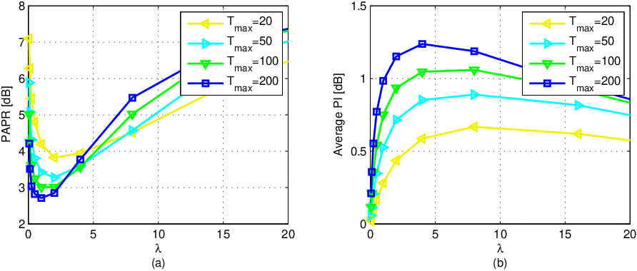
We examine the impact of the choice of the regularization parameter on the PAPR reduction performance. Fig. 5 shows the PAPR and the average power increase (PI) of our proposed method vs. under different choices of , where is fixed to be and the results are obtained over independent runs. From Fig. 5, we observe that our proposed algorithm is able to achieve a substantial PAPR reduction when is within the range . Moreover, when , increasing the maximum number of iterations in general reduces the PAPR but results in a larger power increase (PI). Therefore, to reduce the PI, one can terminate the iterative process as long as the solution meets the specified PAPR requirement. Also, an excessively large value of leads to bad solutions because the data fitting term becomes less influential, and as a result, the transmitted signal could be far away from the desired low PAPR solution .
VI Conclusions
We considered the problem of PAPR reduction for large-scale MU-MIMO-OFDM systems. A perturbation-assisted approach was proposed, where carefully devised artificial perturbation signals are added to the precoded signals to reduce the PAPRs of the transmitted signals. Meanwhile, the perturbations signals are constrained to lie within the null-spaces of the associated channel matrices such that they cause no multi-user interference or out-of-band radiations. We formulated the PAPR reduction problem as a convex optimization problem and developed an efficient algorithm by resorting to the variable splitting and the ADMM techniques. Simulations results show that the proposed algorithm achieves remarkable PAPR reduction performance comparable to [15], meanwhile providing a much faster convergence rate.
References
- [1] 3rd Generation Partnership Project (3GPP), “Evolved universal terrestrial radio access (EUTRA); physical channels and modulation (release 10),” 3GPP Technical Specification, TS 36.211 Rev. 10.3.0, Sep. 2011.
- [2] IEEE 802.16 Working Group, “IEEE standard for air interface for broadband wireless access systems,” IEEE 802.16, Aug. 2012.
- [3] IEEE 802.11 Working Group, “Part 11: wireless LAN medium access control (MAC) and physical layer (PHY) specifications, amendment 5: enhancements for higher throughput,” IEEE 802.11n, Sept. 2009.
- [4] R. O¡¯Neill and L. B. Lopes, “Envelope variations and spectral splatter in clipped multicarrier signals,” in Proc. IEEE PIMRC’95, Toronto, Canada, Sept. 1995, pp. 71–75.
- [5] J. Tellado, “Peak to average power reduction for multicarrier modulation,” PhD thesis (Stanford University, 2000).
- [6] B. S. Krongold and D. L. Jones, “PAR reduction in OFDM via active constellation extension,” IEEE Trans. Broadcasting, vol. 49, no. 3, pp. 258–268, Sept. 2003.
- [7] R. W. Bäuml, R. F. Fischer, and J. B. Huber, “Reducing the peak-to-average power ratio of multicarrier modulation by selected mapping,” IEE Elec. Letters, vol. 32, no. 22, pp. 2056–2057, Oct. 1996.
- [8] S. H. Müller and J. B. Huber, “OFDM with reduced peak-to-average power ratio by optimum combination of partial transmit sequences,” IEE Elec. Letters, vol. 33, no. 5, pp. 368–369, Feb. 1997.
- [9] T. Jiang, Y. Yang, and Y.-H. Song, “Exponential companding technique for PAPR reduction in OFDM systems,” IEEE Trans. Broadcasting, vol. 51, no. 2, pp. 244–248, 2005.
- [10] S. H. Han and J. H. Lee, “An overview of peak-to-average power ratio reduction techniques for multicarrier transmission,” IEEE Wireless Commun., vol. 12, no. 2, pp. 56–65, Apr. 2005.
- [11] R. F. H. Fischer and M. Hoch, “Directed selected mapping for peak-to-average power ratio reduction in MIMO OFDM,” IEE Elec. Letters, vol. 42, no. 2, pp. 1289–1290, Oct. 2006.
- [12] T. Jiang and Y. Wu, “An overview: Peak-to-average power ratio reduction techniques for OFDM signals,” IEEE Trans. Broadcasting, vol. 54, no. 2, pp. 257–268, June 2008.
- [13] T. Tsiligkaridis and D. L. Jones, “PAPR reduction performance by active constellation extension for diversity MIMO-OFDM systems,” J. Electrical and Computer Eng., Sept. 2010.
- [14] H. Prabhu, O. Edfors, J. Rodrigues, L. Liu, and F. Rusek, “A low-complex peak-to-average power reduction scheme for OFDM based massive MIMO systems,” in Communications, Control and Signal Processing (ISCCSP), 2014 6th International Symposium on, Athens, Greece, 2014.
- [15] C. Studer and E. G. Larsson, “PAR-aware large-scale multi-user MIMO-OFDM downlink,” IEEE J. Sel. Areas Commun., vol. 31, no. 2, pp. 303–313, Feb. 2013.
- [16] H. Bao, J. Fang, H. Li, Z. Chen, and S. Li, “An efficient Bayesian PAPR reduction method for OFDM-based massive MIMO systems,” IEEE Trans. Wireless Communications, vol. 15, no. 6, pp. 4183–4195, June 2016.
- [17] J. Chen, C. Wang, K. Wong, and C. Wen, “Low-complexity precoding design for massive multiuser MIMO systems using approximate message passing,” IEEE Trans. Vehicular Technology, vol. PP, no. 99, pp. 1–8, Jul. 2015.
- [18] R. F. H. Fischer, Precoding and Signal Shaping for Digital Transmission. Wiley, New York, 2002.
- [19] C. Tellambura, “Computation of the continuous-time PAR of an OFDM signal with BPSK subcarriers,” IEEE Commun. Lett., vol. 5, no. 5, pp. 185–187, May 2001.
- [20] N. Parikh and S. Boyd, “Proximal algorithms,” Foundations and Trends in optimization, vol. 1, no. 3, pp. 123–231, 2013.
- [21] C. Studer, T. Goldstein, W. Yin, and R. G. Baraniuk, “Democratic representations,” arXiv preprint arXiv:1401.3420, 2014.
- [22] S. Boyd, N. Parikh, E. Chu, B. Peleato, and J. Eckstein, “Distributed optimization and statistical learning via the alternating direction method of multipliers,” Foundations and Trends in Machine Learning, vol. 3, no. 1, pp. 1–122, 2011.