Reliability of the two-point measurement of the spatial correlation length from Gaussian-shaped fluctuating signals in fusion-grade plasmas

In this section, we analytically derive the correlation value between the two spatial positions at $x=x_{a}$ and $x=x_{b}$ at the correlation time delay $\tau=0$ (as we are interested in obtaining the correlation length of the fluctuating signals) and its associated variance.

To analytically derive the correlation function following Kim et al. [23], $\Delta L$ and $\Delta T$ are assumed to be infinitely large compared to $\lambda_{x}$ and $\tau_{\text{life}}$. A correlation value $C_{a,b}$ between $x=x_{a}$ and $x_{b}$ is calculated as $\text{E}\left[S_{a}\left(t\right)S_{b}\left(t\right)\right]$, where $\text{E}\left[\>\right]$ is the time averaging operator over the ‘sub-time window’ whose size is set by $\Delta T_{\text{sub}}$. Then, the ensemble averaged correlation value $\left<C_{a,b}\right>$ is [23]

where the approximation in the last line is valid for $\tau_{\text{ac}}/\Delta T_{\text{sub}}\ll 1$. $\Delta T_{\text{sub}}$ is much smaller than $\Delta T$ allowing many of $\Delta T_{\text{sub}}$ to exist within $\Delta T$ (for an ensemble average [23]) but still much larger than $\tau_{\text{ac}}$, the usual auto-correlation time of the fluctuating signal in the lab frame defined as [30]

Note that the square of the fluctuation level $\left<C_{a,a}\right>$ is $\sim\mathcal{O}\left(A^{2}\right)$ for the spatio-temporal filling factor $F\sim\mathcal{O}\left(1\right)$.

The correlation values, i.e., $C_{a,b}$, have a certain distribution resulting from the fact that the amplitude ($A_{i}$) and the spatio-temporal location ($x_{i}$ and $t_{i}$) of the eddies are randomly distributed. This distribution gives us randomness in $C_{a,b}$, i.e., the variance $\sigma^{2}_{{}_{C_{a,b}}}$ (see Appendix A), which is

where the approximation is valid for $\Delta L\gg\lambda_{x}$, $\Delta T\gg\Delta T_{\text{sub}}\gg\tau_{\text{life}}\text{ (or }\tau_{\text{ac}}\text{)}$, and $N\gg 1$ with the condition of spatio-temporal filling factor $F\sim\mathcal{O}\left(1\right)$ consistent with the assumptions we made to obtain $\left<C_{a,b}\right>$ in Eq. (4). Note that large $N$ is, in fact, a consequence of having $F\sim\mathcal{O}\left(1\right)$ with large $\Delta L$ and $\Delta T$.

We now calculate the normalized correlation functions with and without noise and their associated variances. Again, we are interested in the correlation value between the two spatial points $x_{a}$ and $x_{b}$ at the correlation time delay $\tau=0$. Although the correlation length can be estimated with the ensemble averaged correlation value derived above, we derive the normalized correlation value because the normalized one estimates the correlation length more accurately (smaller bias error) and reliably (smaller variance) compared to the unnormalized one, which we show later in Sec. III.2.

The ensemble averaged normalized correlation value without noise, $\left<\overline{C}_{a,b}\right>$, is

where $\delta_{a}=\sqrt{C_{a,a}}$ and $\delta_{b}=\sqrt{C_{b,b}}$ are the fluctuation levels at the locations $x=x_{a}$ and $x_{b}$, respectively. We have denoted this fluctuation level as $\delta_{f}$ and assumed $\delta_{a}\approx\delta_{f}$ and $\delta_{b}\approx\delta_{f}$ based on the homogeneity of the data. Note that $\left<\delta_{f}^{2}\right>=\pi A^{2}F$ from Eq. (4). The validity of the approximation in the second line of Eq. (7) is provided in Appendix B.

As for the case of $C_{a,b}$, $\overline{C}_{a,b}$ also has a distribution resulting in a finite variance solely due to the randomness of the eddies. This variance denoted as $\sigma^{2}_{{}_{\overline{C}_{a,b}}}$ is

The detailed derivation of $\sigma^{2}_{{}_{\overline{C}_{a,b}}}$ and assumptions we made are provided in Appendix C.1.

Let us now consider the signal with uncorrelated noise. Our model signal with noise $S_{a}^{\text{noise}}\left(t\right)$ is, then,

where $n_{a}\left(t\right)$ is the noise as a function of time at $x=x_{a}$. A normalized correlation value with noise ${\overline{C}_{a,b}^{\text{noise}}}^{\star}$ between the signals from two spatial positions $x_{a}$ and $x_{b}$ is

Note that $\text{E}\left[n_{a}(t)n_{b}(t)\right]=0$ unless $x_{a}=x_{b}$ due to the uncorrelated noise assumption. The normalized correlation value at $x_{a}=x_{b}$ is by definition one whether or not there exists noise, i.e., $\overline{C}_{a,a}=1$ and ${\overline{C}_{a,a}^{\text{noise}}}^{\star}=1$. It is obvious that the effect of $\text{E}\left[n_{a}(t)n_{b}(t)\right]$ on ${\overline{C}_{a,b}^{\text{noise}}}^{\star}$ for $x_{a}=x_{b}$ can be removed for our model signal, but it is also possible to do so with experimental data by considering the auto-correlation function as a function of the correlation time delay $\tau$ [31]. The idea is, basically, interpolating the auto-correlation signal around $\tau=0$ to eliminate the effect of $\text{E}\left[n_{a}(t)n_{b}(t)\right]$ present only around very short interval of $\tau=0$.

Once we remove the noise effect at $x_{a}=x_{b}$ both for our model data and experimental data, we can define $\overline{C}_{a,b}^{\text{noise}}$ as

where we assumed the the noise level $\delta_{n}$ is homogeneous as is the case for $\delta_{f}$. Then, the ensemble averaged normalized correlation value with noise is

The first line equality is owing to the fact the normalized correlation value $C_{a,b}/\delta_{f}^{2}$ is not correlated with a function of fluctuation levels, i.e., $\delta_{f}^{2}/\left(\delta_{f}^{2}+\delta_{n}^{2}\right)$. The second line approximation is based on the same rationale for $\left<\frac{C_{a,b}}{\delta_{f}^{2}}\right>\approx\frac{\left<C_{a,b}\right>}{\left<\delta_{f}^{2}\right>}$ in Eq. (7) (see Appendix B). Notice that the effective role of the noise is to decrease the normalized correlation value, and it is not even unity at $x_{a}=x_{b}$, rather it is a function of fluctuation($\delta_{f}$)-to-noise($\delta_{n}$) ratio (FNR).

The variance $\sigma^{2}_{{}_{\overline{C}_{a,b}^{\text{noise}}}}$ of the ensemble averaged normalized correlation value with noise calculated in Appendix C.2 is

where $\sigma^{2}_{\delta_{f}^{2}}$ and $\sigma^{2}_{\delta_{n}^{2}}$ are the variances of $\delta_{f}^{2}$ and $\delta_{n}^{2}$, respectively. Since $\delta_{f}^{2}=C_{a,a}$, we have $\sigma^{2}_{\delta_{f}^{2}}=\sigma^{2}_{{}_{C_{a,a}}}$ which can be calculated using Eq. (6).

Note that Eq. (12) and Eq. (II.2) which are the ensemble averaged normalized correlation value and its variance with noise, respectively, become Eq. (7) and Eq. (8) for $\delta_{n}^{2}=0$, and none of these equations contain unknowns for our model fluctuation data.

To confirm that the analytically derived unnormalized and normalized correlation values and their associated variances are indeed correct, we generate 50 sets of 1D synthetic data based on Eq. (1) and Eq. (2). These sets of synthetic fluctuation data are generated such that they are guaranteed to be homogeneous and stationary [23].

The basic properties of each set of the synthetic data are: the characteristic spatial scale $\lambda_{x}=0.3$ m, the characteristic temporal scale $\tau_{\text{life}}=15\penalty\ \mu$s, the velocity of the eddies $v=5,000$ m/s, the total time window for the data $\Delta T=15,000\penalty\ \mu$s with the sub-time window $\Delta T_{\text{sub}}=585\penalty\ \mu$s (giving 25 sub-time windows) and the spatial domain size $\Delta L=2.7$ m. To make sure that the synthetic data are homogeneous, $\delta_{f}^{2}$ is kept to be constant in space as well as satisfying the criteria on the domain size according to reference [23].

From the synthetic data we estimate the correlation value $\left<C_{a,b}\right>^{*}$ (we use a superscript asterisk to denote that it is estimated with the synthetic data) and its standard deviation, i.e., square root of the variance, $\sigma_{{}_{C_{a,b}}}^{*}$ as

where the superscripts $i$ and $j$ denote the $i^{\text{th}}$ set and the $j^{\text{th}}$ sub-time window within a set of the synthetic data, respectively. Here, $C_{a,b}^{ij*}$ is estimated as

Figure 1(a) shows analytically calculated $\left<C_{a,b}\right>$ (red line) using Eq. (4) and $\left<C_{a,b}\right>^{*}$ (blue line) using Eq. (14) on the synthetic data as a function of $\Delta x=\left|x_{a}-x_{b}\right|$. They show a good agreement. The error bars on $\left<C_{a,b}\right>^{*}$ are $\sigma_{{}_{C_{a,b}}}^{*}$. Furthermore, Figure 1(b) illustrates a good agreement within the $95$% confidence interval between the analytically calculated $\sigma_{{}_{C_{a,b}}}$ (red line) using Eq. (6) and estimated $\sigma_{{}_{C_{a,b}}}^{*}$ from the synthetic data using Eq. (14) as a function of $\Delta x$.

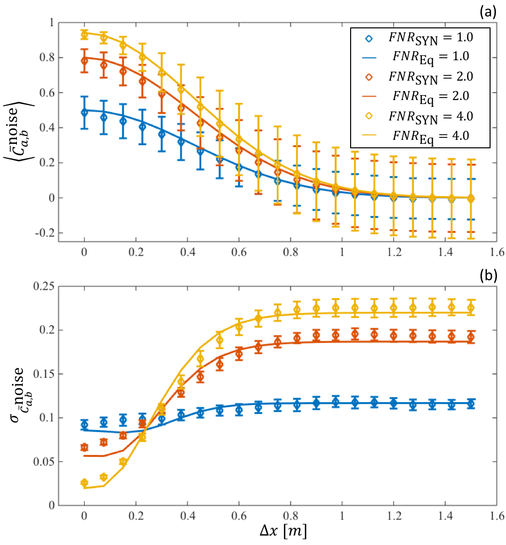
Similar comparisons are shown in Figure 2 for the normalized correlation values with various fluctuation-to-noise ratios (FNR=$\delta_{f}/\delta_{n}$): FNR = $1.0$ (blue), $2.0$ (red) and $4.0$ (yellow). Normalized correlation values and their standard deviations with noise, $\left<\overline{C}_{a,b}^{\text{noise}}\right>$ and $\sigma_{{}_{\overline{C}_{a,b}^{\text{noise}}}}$, are calculated using Eq. (12) and Eq. (II.2); while they are also obtained from the synthetic data, $\left<\overline{C}_{a,b}^{\text{noise}}\right>^{*}$ and $\sigma^{*}_{{}_{\overline{C}_{a,b}^{\text{noise}}}}$, using Eq. (14) with normalized $C_{a,b}^{ij*}$. Again, we find good agreements between the analytical and numerical results.

Note that the value of $\left<\overline{C}_{a,b}^{\text{noise}}\right>$ with $x_{a}=x_{b}$, i.e., $\Delta x=0$ is $\left<\delta_{f}^{2}\right>/\left(\left<\delta_{f}^{2}\right>+\left<\delta_{n}^{2}\right>\right)$ according to Eq. (12). Thus, we expect this value to be $0.50$, $0.80$ and $0.94$ for FNR = $1.0$, $2.0$ and $4.0$, respectively. These values coincide with the results from synthetic data which are obtained by removing the noise in the signal by using the interpolation technique around the correlation time delay $\tau=0$ of the auto-correlation function [31] as mentioned earlier.

As vindicated by the numerical results, we can use the analytically obtained normalized correlation values with and without noise and their associated variances to examine the accuracy (bias error) and reliability (variance) of the two-point measurement of the spatial correlation length.

To be able to calculate $\mu_{\ell_{x}}$ and $\sigma^{2}_{\ell_{x}}$, we need to know the probability density function of $\left<\overline{C}_{a,b}^{\text{noise}}\right>$, i.e., $p\left(C_{1}\right)$ and $p\left(C_{2}\right)$ in Eq. (III). The variance of the ensemble averaged correlation value is $1/M$ times the variance of the correlation value where $M$ is the sample number, i.e., the number of sub-time windows used to measure the ensemble average of the correlation value. Owing to the central limit theorem, this probability density function, $p\left(C_{1}\right)$ or $p\left(C_{2}\right)$, is a normal distribution function with the mean of $\left<\overline{C}_{a,b}^{\text{noise}}\right>$ and the standard deviation of $\sigma_{{}_{\overline{C}_{a,b}^{\text{noise}}}}/\sqrt{M}$ which can be estimated either analytically or numerically with the synthetic data.

Once we have the probability density functions $p\left(C_{1}\right)=P\left(\left<\overline{C}_{a,a}^{\text{noise}}\right>\right)$ and $p\left(C_{2}\right)=P\left(\left<\overline{C}_{a,b}^{\text{noise}}\right>\right)$ either from the analytic results or numerical synthetic data, a Monte-Carlo method by generating $10,000$ samples from these probability density functions is used to generate a histogram of the correlation length normalized to the true correlation length $\ell_{x}^{\text{true}}=\sqrt{2}\lambda_{x}$ as a function of the separation distance between the two measured positions $\Delta x$ normalized to the true correlation length $\ell_{x}^{\text{true}}$ as well.

This histogram is, then, used to estimate the mean $\mu_{\ell_{x}}$ and the variance $\sigma^{2}_{\ell_{x}}$ of the two-point correlation length measurements. Note that we ignore the case of $C_{1}\leq C_{2}$ which corresponds to $\ell_{x}=\infty$. Nevertheless, if $C_{1}\leq C_{2}$ occurs frequently, indicating that the correlation length $\ell_{x}$ is much larger than the separation distance of the two measurement positions, such a signature will be shown as a large variance according to Eq. (III) and Eq. (III). Here, we examine two major factors that affect the quality of the correlation length measurements: 1) size of the total time window and 2) noise level.

To quantify how the size of the total time window affects the measured correlation length, we generate three sets of synthetic data with $\lambda_{x}=0.3$ m, $\tau_{\text{life}}=15\penalty\ \mu$s, $v=5,000$ m/s and $\Delta T_{\text{sub}}=585\penalty\ \mu$s at the fixed FNR of $0.5$, whereas $\Delta T$ are set to be $10,000\penalty\ \mu$s, $30,000\penalty\ \mu$s and $50,000\penalty\ \mu$s. Figure 4 shows the histograms of the obtained correlation length with the $p\left(C_{1}\right)$ and $p\left(C_{2}\right)$ from the analytic results (left panels) and the synthetic data (right panels). Based on these histograms, we finally obtain the average and standard deviation of the correlation length (normalized to $\ell_{x}^{\text{true}}$) as a function of $\Delta x/\ell_{x}^{\text{true}}$ as shown in Figure 5. Although Figure 5 is more succinct than Figure 4, it is better to consider Figure 4 because the first ($\mu_{\ell_{x}}$) and second ($\sigma^{2}_{\ell_{x}}$) moments become less representative as the histogram deviates from a normal distribution, especially for small and large $\Delta x/\ell_{x}^{\text{true}}$.

The similar trend between the analytic and numerical results shows that increasing the size of the total window decreases the standard deviation of the measurements, and the two-point correlation length measurement becomes less reliable if the separation distance between the two measured points are either smaller than or more than two times larger than the actual correlation length of the fluctuation data.

Next, we examine the effect of noise level, i.e., the fluctuation-to-noise ratio (FNR), on the two-point correlation length measurements. Three sets of synthetic data with $\lambda_{x}=0.3$ m, $\tau_{\text{life}}=15\penalty\ \mu$s, $v=5,000$ m/s, $\Delta T=15,000\penalty\ \mu$s and $\Delta T_{\text{sub}}=585\penalty\ \mu$s are generated with different values of FNR: $1.0$, $2.0$ and $4.0$. Figure 6 shows the histograms of the obtained correlation length using the analytic results (left panel) and synthetic data (right panel), whereas the average and standard deviation of the correlation length is shown in Figure 7.

We find that the lower limit on the $\Delta x/\ell_{x}^{\text{true}}$ is dependent on the FNR; while the upper limit is not. This observation can be explained based on Figure 2. We see that the standard deviation levels are larger at small $\Delta x$ for the smaller FNR. This results in a larger value on the lower limit of $\Delta x/\ell_{x}^{\text{true}}$ with the smaller FNR. In addition, larger standard deviation at the small $\Delta x/\ell_{x}^{\text{true}}$ is more probable to have $C_{1}\leq C_{2}$ in Eq. (III). Figure 2 also shows that although the standard deviation levels are larger with the larger FNR at large $\Delta x$, they are smaller at $\Delta x=0$. Therefore, we observe similar upper limit on $\Delta x/\ell_{x}^{\text{true}}$ for the investigated FNR cases.

The variance of the correlation length $\sigma^{2}_{\ell_{x}}$ is a function of $p\left(C_{1}\right)$ and $p\left(C_{2}\right)$ as shown in Eq. (III), i.e., the narrower the $p\left(C_{1}\right)$ and $p\left(C_{2}\right)$, the smaller the variance. Considering an extreme case of absolutely no noise, we see that $p\left(C_{1}\right)$ is a delta function, i.e., no variance, for the normalized correlation function (see Eq. (8)) while it always has a non-zero width, i.e., non-zero variance, for the unnormalized correlation function (see Eq. (6)). Figure 8 shows the unnormalized (blue) and normalized correlation functions with no noise (red) and FNR=4.0 (yellow) as a function of $\Delta x/\ell_{x}^{\text{true}}$ calculated with the analytic results. Here, the error bars represent the standard deviation of the mean, i.e., $1/\sqrt{M}$ times the standard deviation of the correlation value; thus, they provide approximate widths of $p\left(C_{1}\right)$ and $p\left(C_{2}\right)$. Direct comparison of the widths of $p\left(C_{2}\right)$ between unnormalized and normalized correlation functions can be tricky as they are functions of $\Delta x$, but the very small width of the $p\left(C_{1}\right)$ at $\Delta x=0$ for the normalized correlation function, in general, provides better correlation length measurements compared to the unnormalized correlation function.

Figure 9 shows the average and standard deviation of the correlation length estimated with the unnormalized (blue) and normalized correlation functions without noise (red) and with the noise level of FNR=4.0 (yellow) with the analytic results as in Figure 8. We see that the normalized correlation function provides smaller standard deviation and bias error of the measured correlation length especially for $\Delta x\leq\ell_{x}^{\text{true}}$.

Reliability and accuracy of the two-point correlation length measurement have been examined analytically and numerically. We now apply the two-point correlation length measurement on the density fluctuation data experimentally obtained via the BES system [19] installed in KSTAR.

Since the ‘true’ correlation length of the fluctuation data are not available, we estimate the correlation length using the four points (poloidally aligned four detectors) denoted as $\ell_{\theta\text{(4 points)}}$ and treat this value as the ‘true’ correlation length. Figure 10 shows an example of four-point measurement of the correlation values (blue) at the time delay $\tau=0$. Note that correlation values for $\Delta x<0$ are just copies of the values from $\Delta x>0$ to aid visualization. Gaussian fitting (red) to the correlation values provides the correlation length $\ell_{\theta\text{(4 points)}}$.

Then, we estimate the correlation length using only two measurement points denoted as $\ell_{\theta\text{(2 points)}}$. Figure 11 shows $\ell_{\theta\text{(2 points)}}/\ell_{\theta\text{(4 points)}}$ as a function of $\Delta x/\ell_{\theta\text{(4 points)}}$ for different sizes of the total time window $\Delta T=10$ ms (blue), $30$ ms (red) and $50$ ms (yellow). The result is quantitatively similar to Figure 4 (or Figure 5), i.e., results obtained analytically and numerically: two-point correlation length measurements are not biased for $1\leq\Delta x/\ell_{\theta\text{(4 points)}}\leq 2$, and a larger size of total time window provides smaller variance.

References

- [1] J. Meinecke, P. Tzeferacos, A. Bell, R. Bingham, R. Clarke, E. Churazov, R. Crowston, H. Doyle, R. P. Drake, R. Heathcote, M. Koenig, Y. Kuramitsu, C. Kuranz, D. Lee, M. MacDonald, C. Murphy, M. Notley, H.-S. Park, A. Pelka, A. Ravasio, B. Reville, Y. Sakawa, W. Wan, N. Woolsey, R. Yurchak, F. Miniati, A. Schekochihin, D. Lamb, and G. Gregori, Proc. Nat. Acad. Sci. USA 112, 8211 (2015).
- [2] B. Carreras, IEEE Trans. Plasma Sci. 25, 1281 (1997).
- [3] N. Iwama, Y. Ohba, and T. Tsukishima, J. Appl. Phys. 50, 3197 (1979).
- [4] J. M. Beall, Y. C. Kim, and E. J. Powers, J. Appl. Phys. 53, 3933 (1982).
- [5] T. S. Horbury, in Cluster II Workshop: Multiscale/Multipoint Plasma Measurements, edited by R. A. Harris (2000).
- [6] G. Taylor, Proc. R. Soc. London A164, 476 (1938).
- [7] P. Goldreich and S. Sridhar, Astrophys. J. 438, 763 (1995).
- [8] J. Cho and A. Lazarian, Astrophys. J. 615, L41 (2004).
- [9] A. A. Schekochihin, S. C. Cowley, W. Dorland, G. W. Hammett, G. G. Howes, E. Quataert, and T. Tatsuno, Astrophys. J. Suppl. 182, 310 (2009).
- [10] S. V. Nazarenko and A. A. Schekochihin, J. Fluid Mech. 677, 134 (2011).
- [11] T. S. Horbury, M. Forman, and S. Oughton, Phys. Rev. Lett. 101, 175005 (2008).
- [12] J. J. Podesta, Astrophys. J. 698, 986 (2009).
- [13] R. T. Wicks, T. S. Horbury, C. H. K. Chen, and A. A. Schekochihin, Mon. Not. R. Astron. Soc. 407, L31 (2010).
- [14] M. Barnes, F. I. Parra, E. G. Highcock, A. A. Schekochihin, S. C. Cowley, and C. M. Roach, Phys. Rev. Lett. 106, 175004 (2011).
- [15] Y.-c. Ghim, A. A. Schekochihin, A. R. Field, I. G. Abel, M. Barnes, G. Colyer, S. C. Cowley, F. I. Parra, D. Dunai, S. Zoletnik, and the MAST Team, Phys. Rev. Lett. 110, 145002 (2012).
- [16] C. P. Ritz, E. J. Powers, T. L. Rhodes, R. D. Bengtson, K. W. Gentle, H. Lin, P. E. Phillips, A. J. Wootton, D. L. Brower, N. C. Luhmann, W. A. Peebles, P. M. Schoch, and R. L. Hickok, Rev. Sci. Instrum. 59, 1739 (1988).
- [17] D. L. Winslow, R. D. Bengtson, B. Richards, and W. A. Craven, Rev. Sci. Instrum. 68, 396 (1997).
- [18] H. Thomsen, M. Endler, J. Bleuel, A. V. Chankin, S. K. Erents, G. F. Matthews, and C. to the EFDA-JET workprogramme, Phys. Plasmas 9, 1233 (2002).
- [19] M. Lampert, G. Anda, A. Czopf, G. Erdei, D. Guszejnov, Á. Kovácsik, G. I. Pokol, D. Réfy, Y. U. Nam, and S. Zoletnik, Rev. Sci. Instrum. 86, 073501 (2015).
- [20] W. Lee, I. Hong, J. Leem, M. Kim, Y. Nam, G. S. Yun, H. K. Park, Y. G. Kim, K. W. Kim, C. W. Domier, and N. C. J. Luhman, J. Instrum. 7, C01070 (2012).
- [21] B. Tal, A. Bencze, S. Zoletnik, G. Veres, and G. Por, Phys. Plasmas 18, 122304 (2011).
- [22] Y.-c. Ghim, A. R. Field, D. Dunai, S. Zoletnik, L. Bardóczi, A. A. Schekochihin, and the MAST Team, Plasma Phys. Controlled Fusion 54, 095012 (2012).
- [23] J. Kim, M. Fox, A. Field, Y. Nam, and Y.-c. Ghim, Comput. Phys. Commun. 204, 152 (2016).
- [24] R. J. Fonck, G. Cosby, R. D. Durst, S. F. Paul, N. Bretz, S. Scott, E. Synakowski, and G. Taylor, Phys. Rev. Lett. 70, 3736 (1993).
- [25] G. R. McKee, C. Fenzi, R. J. Fonck, and M. Jakubowski, Rev. Sci. Instrum. 74, 2014 (2003).
- [26] Y.-c. Ghim, A. R. Field, A. A. Schekochihin, E. G. Highcock, C. Michael, and the MAST Team, Nucl. Fusion 54, 042003 (2014).
- [27] J. E. Maggs and G. J. Morales, Phys. Rev. Lett. 107, 185003 (2011).
- [28] G. Hornung, B. Nold, J. E. Maggs, G. J. Morales, M. Ramisch, and U. Stroth, Phys. Plasmas 18, 082303 (2011).
- [29] D. A. D’Ippolito, J. R. Myra, and S. J. Zweben, Phys. Plasmas 18, 060501 (2011).
- [30] A. Bencze and S. Zoletnik, Phys. Plasmas 12, 052323 (2005).
- [31] S. Zoletnik, S. Fiedler, G. Kocsis, G. K. McCormick, J. Schweinzer, and H. P. Winter, Plasma Phys. Controlled Fusion 40, 1399 (1998).
- [32] N. L. J. Regina C. Elandt-Johnson, Survival Models and Data Analysis (Wiley, 1999).
- [33] L. A. Goodman, J. Am. Stat. Assoc. 55, 708 (1960).