Effective time reversal and echo dynamics in the transverse field Ising model

During the last decades enormous advances in the experimental realisation of highly controllable quantum simulators [1, 2, 3, 4] have triggered a lot of activity in theoretically investigating the out of equilibrium dynamics of quantum many-body systems. In particular the equilibration of closed many-body systems and the process of thermalisation as fundamental questions of quantum statistical mechanics aroused a lot of interest [5, 6, 7, 8, 9, 10, 11, 12, 13, 14]. Nevertheless, albeit being intimately related to thermalisation the question of irreversibility in quantum many-body systems has to date hardly been addressed.

In the context of classical systems this question was already discussed during the development of thermodynamics. Regarding Boltzmann’s H-theorem [15] Loschmidt pointed out that in his derivation of the Second Law Boltzmann had obviously broken the time reversal invariance of the underlying microscopic laws of motion[16]. Specifically, he argued that if one performs an effective time reversal on a classical gas by inverting the velocities of all particles at some point in time the system must necessarily return to its initial state after twice that time. With this example at hand the emergence of irreversibility in classical systems is nowadays easily understood: A system with sufficiently many degrees of freedom will generically exhibit chaotic dynamics and therefore any time reversal operation will be practically infeasible due to the exponential sensitivity of the dynamics to inevitable errors. This is also a way to understand the loss of information about the initial state during the time evolution, which is essential for thermalisation. In a chaotic many-body system with irreversible dynamics there is no realisable protocol that would allow to return it to the initial state.

Referring to the knowledge about classical irreversibility Peres suggested to study the Loschmidt echo

in order to quantify irreversibility of quantum systems [17]. The Loschmidt echo is the overlap of the initial state with the forward and backward time evolved state when including a small deviation $\epsilon V$ in the time evolution operator of the backwards evolution. As such it quantifies how well the initial state is resembled after an imperfect effective time reversal. The Loschmidt echo turned out to be a very interesting measure when studying systems with few degrees of freedom, exhibiting a variety of possible decay characteristics [18, 19].

However, in generic quantum many-body systems the Loschmidt echo is not a measurable quantity. If the prerequisite of the Eigenstate Thermalisation Hypothesis (ETH) [20, 21, 22] pertains, which all numerical evidence indicates [7, 23, 24], then expectation values of local observables $O_{E}=\langle E|\hat{O}|E\rangle$ are smooth functions of the eigenstate energy $E$. This means that even orthogonal states cannot necessarily be distinguished experimentally. This argument carries over to integrable systems when the observable expectation value is considered as a function of all integrals of motion instead of only the energy [25]. Therefore a definition of irreversibility with respect to the Loschmidt-echo cannot meaningfully differentiate between reversible and irreversible dynamics in many-body systems. It should also be noted that generally the Loschmidt echo is of large deviation form, $\mathcal{L}(\tau)\sim e^{-Nl(\tau)}$ with some rate function $l(\tau)$, i.e. it is exponentially suppressed with increasing system size $N$.

In our work, when addressing the question of irreversibility in many-body systems we focus on observable echoes that are produced under imperfect effective time reversal, i.e.

We propose a definition of irreversibility based on the decay of the echo peak as the waiting time $\tau$ is increased. With respect to that we consider the dynamics of systems exhibiting an algebraic decay reversible, whereas systems with exponentially or faster than exponentially decaying echo peaks are irreversible.

Obviously, echoes in the expectation values of observables will depend on the choice of the observables. Thus, the conclusions that can be drawn regarding the irreversibility of the dynamics will have to be decided on a case by case basis. However, to the best of the current knowledge fundamental issues of thermalisation, in particular the description of stationary expectation values in unitarily evolved pure states after long times by thermal density matrices, can likewise only be understood for specific classes of observables [13, 14].

Recently, an alternative definition for chaos in quantum systems was put forward, which is based on the behaviour of out-of-time-order (OTO) correlators of the form $\langle W(t)V(0)W(t)V(0)\rangle$. These OTO correlators probe a system’s sensitivity to small perturbations [26]. Moreover, they are closely related to the phenomenon of scrambling, i.e. the complete delocalisation of initially local information under time evolution [27]. The relation between both definitions should be investigated systematically in future work.

An important experimental application of effective time reversal are NMR experiments. The dynamics of non-interacting spins can be reverted by the Hahn echo technique [28] or by the application of more sophisticated pulse sequences [29, 30]. Moreover, it is possible to realise effective time reversal in certain dipolar coupled spin systems by the so called magic echo technique [31, 32, 33]. Particularly notable are various experimental and theoretical works on the refocussing of a local excitation by effective time reversal in NMR setups [34, 35, 36, 37]. Besides that we expect that effective time reversal can be realised in quantum simulators [3, 4]; and recently there were proposals for effective time reversal by periodic driving [38] or by spin flips in cold atom setups with spin-orbit coupling [39].

Results for the echo dynamics in many-body systems might also be interesting from other points of view. For example, there are proposals for the identification of many-body localised phases using spin echoes [40] or for the certification of quantum simulators using effective time reversal [41].

In this letter we report results for effective time reversal in the transverse field Ising model (TFIM). This simple model Hamiltonian is diagonal in terms of fermionic degrees of freedom and all quantities of interest can be computed analytically in the thermodynamic limit. Thus, it has well known properties and, in particular, the stationary state it approaches in the long time limit is well understood [10, 42]. As such the TFIM is ideally suited as a starting point to study irreversibility theoretically from the aforementioned point of view. On top of this, the TFIM has been realised experimentally in circuit QED [43].

The Ising model in a transverse magnetic field is defined by the Hamiltonian

where $S_{i}^{x/z}$ denotes the Pauli spin operators acting on lattice site $i$, $N$ the number of lattice sites, and $h$ the magnetic field strength [44]. For our purposes we consider periodic boundary conditions. A Jordan-Wigner transform allows to map this spin Hamiltonian to a quadratic Hamiltonian in momentum space

with fermionic operators $c_{k}^{\dagger},c_{k}$ and coefficient functions $d_{k}^{y}(g)=\sin(k)/2$ and $d_{k}^{z}(g)=g-\cos(k)/2$, where $g=h/J$. The Bogoliubov rotation

with Bogoliubov angle $\theta_{k}^{g}=\arctan\left(d_{k}^{y}/d_{k}^{z}(g)\right)$ diagonalises the Hamiltonian yielding

with energy spectrum $\epsilon_{k}^{g}=J\sqrt{d_{k}^{y}(g)^{2}+d_{k}^{z}(g)^{2}}$. The gap closing point at $g=1/2$ indicates the quantum phase transition between paramagnet and ferromagnet.

Above a family of unitary matrices,

with the Pauli matrices $\sigma^{\alpha}$ was introduced for later convenience.

After mapping the spin degrees of freedom to free fermions expectation values of many observables are – thanks to Wick’s theorem – given in terms of block Toeplitz (correlation) matrices $\Gamma_{ij}\equiv\Gamma_{(i-j)}$, where

with

and Majorana operators $a_{i}=c_{i}^{\dagger}+c_{i},b_{i}=\mathrm{i}(c_{i}^{\dagger}-c_{i})$ [45, 46, 47, 48, 49]. Here $\langle\cdot\rangle$ denotes the expectation value for a given state $|\psi\rangle$, i.e. $\langle\cdot\rangle\equiv\langle\psi|\cdot|\psi\rangle$. Since, due to translational invariance,

where $a_{k}=\frac{1}{\sqrt{N}}\sum_{l}e^{-\mathrm{i}kl}a_{l}$ and $b_{k}=\frac{1}{\sqrt{N}}\sum_{l}e^{-\mathrm{i}kl}b_{l}$, the Toeplitz matrix $\Gamma_{ij}$ is fully determined by its symbol

via $\Gamma_{l}=\sum_{k}e^{-\mathrm{i}kl}\hat{\Gamma}_{k}$.

For our purposes we consider the transverse magnetisation

and the longitudinal spin-spin correlation

where $\operatorname{Pf}[\cdot]$ denotes the Pfaffian and $\Gamma^{n}$ is the correlation matrix consisting of blocks $\Gamma_{ij}$ with $|i-j|<n$ (cf. eq. (8)). Moreover, we will study the entanglement entropy $S_{n}$ of a strip $A_{n}$ of $n$ adjacent spins with the rest of the system, which is given by

where $\rho_{A_{n}}$ is the reduced density matrix of the subsystem $A_{n}$ and $\nu_{l}$ are the eigenvalues of $\Gamma^{n}$ [50, 51].

In the following we will be interested in time evolution which is induced by quenching the magnetic field $g$ at $t=0$. This means the initial state $|\psi_{0}\rangle$ is the ground state of the Hamiltonian $H(g_{0})$ and for $t>0$ the time evolution is driven by a Hamiltonian $H(g)$ with $g\neq g_{0}$. To compute the time evolution for this protocol it is convenient to introduce operators

in terms of which the correlators (9) and (10) are $\mathrm{i}\langle a_{i}a_{j}\rangle=\mathrm{i}\langle\omega_{i}^{+}\omega_{j}^{+}\rangle$ and $\mathrm{i}\langle a_{i}b_{j}\rangle=-\langle\omega_{i}^{+}\omega_{j}^{-}\rangle$ . $\Gamma^{n}$ is then fully determined by the correlation matrix

where $\langle\cdot\rangle_{t}$ is the expectation value with respect to the time evolved state $|\psi(t)\rangle$. For the abovementioned quench the expectation values with $|\psi(t)\rangle=\exp\left(-\mathrm{i}H(g)t\right)|\psi_{0}\rangle$ can be evaluated [52], yielding

where $\tilde{U}_{k}(t)=\sqrt{2}R^{y}\left(\frac{\pi}{2}\right)R^{x}(\theta_{k}^{g})R^{z}(2\epsilon_{k}^{g}t)R^{x}(\phi_{k}^{g,g_{0}})$ with $R^{\alpha}(\phi)$ as defined in eq. (7) and $\phi_{k}^{g,g_{0}}\equiv\theta_{k}^{g}-\theta_{k}^{g_{0}}$. In the following we will employ straightforward generalisations of this formalism for situations of imperfect effective time reversal, generally yielding coefficients $\Sigma_{\alpha}^{k}(t)\equiv\Sigma_{\alpha}^{k}(t,g_{0},g,\ldots)$ with which

where $\sigma^{\alpha}$ denote the Pauli matrices. Although derived straightforwardly, the expressions for $\Sigma_{\alpha}^{k}(t)$ become very lengthy for the time reversal protocols under consideration in this work. The full expressions can be found in the appendix.

In the following we will study the resemblance of a time evolved state to the initial state when different kinds of imperfect effective time reversal are employed at $t=\tau$. For this purpose we compute different time dependent quantities $X_{t}$, namely observables and entanglement entropy. For $t\to\infty$ these quantities approach a stationary value $X_{\infty}$. However, due to the applied time reversal protocol the deviation $|X_{t}-X_{\infty}|$ will show a distinguished maximum at $t_{e}\approx 2\tau$, which we call the echo peak. We will consider the normalised echo peak height

as measure for the initial state resemblance.

According to eqs. (11), (12), and (20) the quantities of interest will in the thermodynamic limit ($N\to\infty$) be determined by integrals $\int_{-\pi}^{\pi}dke^{-\mathrm{i}nk}\Sigma_{\alpha}^{k}/2\pi$, where the time-dependent parts of $\Sigma_{\alpha}^{k}$ oscillate more and more quickly as function of $k$ with increasing $t$. Therefore, the stationary values $X_{\infty}$ are given by the corresponding integrals over only the time-independent contributions to $\Sigma_{\alpha}^{k}$ [52].

In what follows we discuss three different time reversal protocols, namely time reversal by explicit sign change of the Hamiltonian, $H(g)\to-H(g+\delta g)$, time reversal by application of a Loschmidt pulse $U_{P}$, $H(g)\to U_{P}^{\dagger}H(g)U_{P}$, and a generalised Hahn echo protocol, $H(g)\to H(-g)$. All three protocols yield algebraically decaying or even ever persisting echo peak heights.

As a first echo protocol we consider effective time reversal induced by an explicit sign change of the Hamiltonian at time $\tau$ and a well controlled deviation in the backward evolution through a slight variation $\delta g$ of the magnetic field, i.e. for $t>\tau$

where $g_{\delta}\equiv g+\delta g$ was introduced. The corresponding correlation matrix (20) is given by eqs. (38)-(40) in the appendix.

In order to reliably assess how well an initial state can be recovered by imperfect effective time reversal we choose initial states, which exhibit distinguishable expectation values of some observables. These are ground states of $H(g)$ for $g=0$ or $g\gg 1$, respectively, which show large spin-spin correlations.

Under the time reversal protocol described above the energy spectrum $\epsilon_{k}^{g_{\delta}}$ is deformed as compared to $\epsilon_{k}^{g}$ and, consequently, the quasiparticle velocities, $v_{k}=\frac{d\epsilon_{k}}{dk}$, during forward and backward evolution can differ. Therefore, the closest resemblance of the time evolved state to the initial state does not necessarily occur at $t=2\tau$. This becomes evident in the exemplary time evolution displayed in fig. 1a. In addition to observables fig. 1a shows the time evolution of the rate function of the fidelity, $l(t)=\lim_{N\to\infty}\ln(|\langle\psi_{0}|\psi(t)\rangle|^{2})/N$. A minimum of this quantity corresponds to a large overlap of the time evolved state with the initial state for finite $N$. Note as an aside that the time evolution exhibits dynamical quantum phase transitions, which aroused a lot of interest recently [53], in the forward as well as in the backward evolution.

Let us first consider echoes in the transverse magnetisation. For this observable a stationary phase approximation reveals an algebraic decay of the echo peak height with

where $\kappa_{k^{*}}(\tau)=\cos(2(\epsilon_{k^{*}}^{g}-\nu_{k^{*}}^{g,g_{\delta}}\epsilon_{k^{*}}^{g_{\delta}})\tau+\pi/4)$,

and the echo peak time is $t_{e}=(1+\nu_{k^{*}}^{g,g_{\delta}})\tau$ with

From the stationary phase approximation the onset of the algebraic decay can be expected at $\tau\approx\tau^{*}$ with $\tau^{*}=\left.\frac{d}{dk}\zeta_{k}^{g,g_{\delta},g_{0}}\right|_{k=k^{*}}/\xi_{k^{*}}^{g,g_{\delta}}$. On this timescale the oscillating factor varies so slowly that it can be approximated with $\kappa_{k^{*}}(\tau)\approx 1$. A detailed derivation of this result is given in the appendix. Fig. 2a shows the decay of the echo peak height of the transverse magnetisation as a function of the forward time $\tau$ for three different quenches starting in the paramagnetic phase. In all cases the initial magnetisation is almost perfectly recovered for forward times $\tau\lesssim\tau^{*}$, whereas it decays algebraically for $\tau\gg\tau^{*}$. Moreover, the evaluation of $\beta_{k^{*}}^{g,g_{0},g_{\delta}}$ and $\tau^{*}$ as function of the deviation $\delta g$ yields $\beta_{k^{*}}^{g,g_{0},g_{\delta}}\propto\delta g^{-1/2}$ and $\tau^{*}\propto\delta g^{-1}$ for a wide range of perturbation strengths $\delta g$. As a result, $\beta_{k^{*}}^{g,g_{0},g_{\delta}}(\tau^{*})^{-1/2}$ is almost constant (cf. fig. 2b) meaning that generally a very pronounced echo peak can be expected until the onset of the algebraic decay and the height of which is independent of the imperfection in the backwards evolution. Hence, the echo peak decay is ultimately induced by dephasing due to the deformed spectrum in the backwards evolution.

Fig. 3 shows the longitudinal spin-spin correlation $\rho_{d}^{zz}$ computed according to eq. (15) for different distances $d$. For this quantity we also observe an algebraic decay of the echo peak height, $E_{\tau}^{*}[\rho_{d}^{zz}]\propto\tau^{-1/2}$ for large $\tau$. However, before the onset of the algebraic decay there is a distance-dependent regime of exponential-looking decay, which increases with increasing spin-separation $d$. Similar behaviour is known for the decay of correlation functions after a simple quench without time reversal [10, 49]. In that case the decay law can be rigorously derived by identifying an space-time scaling regime where $v_{\text{max}}t\sim d$ with $v_{\text{max}}$ the maximal propagation velocity. Due to the similar algebraic structure in the echo dynamics we expect a similar explanation for the intermediate regime in the decay of the echo peak of $\rho_{d}^{zz}$ with a different effective velocity $\tilde{v}_{\text{max}}=\underset{k\in[0,\pi]}{\text{max}}\frac{d}{dk}(\epsilon_{k}^{g}-\nu_{k^{*}}^{g,g_{\delta}}\epsilon_{k}^{g_{\delta}})$. At late times all entries of the correlation matrix (8) will just like the transverse magnetisation decay algebraically with exponent $-1/2$, and therefore the leading term of the Pfaffian will decay with the same power law, which explains that $E_{\tau}^{*}[\rho_{d}^{zz}]\propto\tau^{-1/2}$ for $\tilde{v}_{\text{max}}\tau\gg d$. Considering the order parameter $\langle m_{z}\rangle=\lim_{d\to\infty}\rho_{d}^{zz}$, our result implies an exponential decay of the echo peak height for all forward times $\tau\gg 1$ when starting from an ordered state.

Another interesting question is how far the entanglement produced during the time evolution can be reduced again by the effective time reversal protocol. After quenching the magnetic field the entanglement entropy increases until it saturates at a level that is determined by the subsystem size [54]. Therefore, an echo peak $E_{\tau}^{*}[S_{d}]=1$ means that the state $|\psi(t_{e})\rangle$ has the same low entanglement as the initial state, whereas for $E_{\tau}^{*}[S_{d}]<1$ some additional entanglement remains. Fig. 4 displays the echo peak height of the entanglement entropy $S_{n}$ of a subsystem $A_{d}$ consisting of $d$ adjacent spins with the rest of the chain as defined in eq. (16). Again we observe an initial $d$-dependent regime of exponential-looking decay crossing over to algebraic decay with $E_{\tau}^{*}[S_{d}]\propto\tau^{-1/2}$ for $\tau>d/2\tilde{v}_{\text{max}}$.

Another possibility to invert the course of the dynamics in the TFIM is the application of a pulse similar to the $\pi$-pulses applied to the system in a Hahn echo experiment. Consider the Hamiltonian

In terms of the Jordan-Wigner fermions in momentum space this reads

and the structure does not change under Bogoliubov rotation, since $c_{k}^{\dagger}c_{-k}^{\dagger}+c_{-k}c_{k}=\lambda_{k}^{\dagger}\lambda_{-k}^{\dagger}+\lambda_{-k}\lambda_{k}$. The time evolution operator for this Hamiltonian in the diagonal basis is

For a given pulse time $t_{P}$ this operator perfectly inverts the population of modes $k_{n}^{*}$ with $2\alpha t_{P}\sin k_{n}^{*}=(2n+1)\pi/2,n\in\mathbb{Z}$, whereas the population of modes $k_{n}^{\times}$ with $2\alpha t_{P}\sin k_{n}^{\times}=n\pi$ remains unchanged. The population of other modes is partially inverted. Thereby, the evolution of the system under the Hamiltonian (28) for a pulse time $t_{p}$ leads to an imperfect effective time reversal, i.e. $e^{\mathrm{i}H_{P}t_{P}}e^{-\mathrm{i}H\tau}e^{-\mathrm{i}H_{P}t_{P}}=e^{\mathrm{i}(H+\epsilon V)\tau}$, by an imperfect inversion of the mode occupation.

Note that in the notation introduced above the pulse operator in one $k$-sector is $\tilde{U}_{k}^{P}(2\alpha t)\equiv R^{x}(4\alpha t\sin k)^{\dagger}$. The result for the corresponding correlation matrix to this echo protocol is given in eqs. (45)-(47) in the appendix.

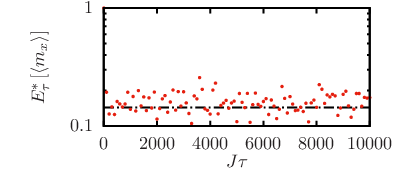
With this protocol the forward and backward time evolution are generated by the same Hamiltonian; hence, the echo peak after time reversal at time $\tau$ appears at $t_{e}=2\tau$, which can be seen in the exemplary time evolution in fig. 1b. In particular, we find that at $t_{e}=2\tau$ the transverse magnetisation can be split into three parts,

where $\langle m_{x}\rangle_{\infty}$ is the stationary value reached at $t\to\infty$, $\langle m_{x}\rangle_{E}$ is an additional $\tau$-independent contribution, and $\langle m_{x}\rangle_{\tau}$ are the time-dependent contributions, which vanish for $\tau\to\infty$. This means we find an echo peak at $t_{e}=2\tau$, which never decays. The residual peak height is given by

An example of this ever persisting echo is depicted in fig. 5, where the dots show the exact result and the dashed line shows the echo peak height expected when only considering the time-independent contributions in eq. (31).

The Hamiltonian of the TFIM (3) allows for an echo protocol very similar to the way the effective time reversal is induced in a Hahn echo experiment [28], namely by a sign inversion of the Zeeman term. For large magnetic fields changing the sign of the field can be considered an effective time reversal with small imperfection given by the Ising term, $\epsilon V=2J\sum_{i}S_{i}^{z}S_{i+1}^{z}$. In contrast to the original Hahn echo setup, where an initial magnetisation decays due to field inhomogeneities, the decay in the TFIM will be due to the coupling of the physical degrees of freedom.

The stationary phase analysis for the echo dynamics under this protocol unveils that it combines two properties of the previously discussed protocols. Since the switching of the magnetic field corresponds to a shift of the energy spectrum, $\epsilon_{k}^{g}=\epsilon_{k+\pi}^{-g}$, the quasiparticle velocities are perfectly inverted, yielding echo peaks at $t_{e}=2\tau$; nevertheless, for large $\tau$ the echo peak height decays algebraically with exponent $-1/2$. A detailed derivation is given in the appendix.

The fact that it is well possible to produce pronounced echoes in the TFIM also after long waiting times matches the absence of thermalisation in the conventional sense. The dynamics of the system is constrained by infinitely many integrals of motion, which keep a lot of information about the initial state. Especially, these integrals of motion determine the stationary value of local observables through the corresponding generalised Gibbs ensemble (GGE) [10], i.e. the reduced density matrix of a strip of length $l$, $\rho_{l}(t)$, converges to a density matrix given by a GGE, $\rho_{GGE,l}$, for $t\to\infty$. Note that the distance of both density matrices decreases as $\mathcal{D}(\rho_{l}(t),\rho_{GGE,l})\propto l^{2}t^{-3/2}$[11], whereas the expectation value of an observable at $t=2\tau$ is determined by $\langle O\rangle_{2\tau}=\text{tr}[O(\tau)\rho(\tau)]$. In the latter expression $\rho(\tau)=e^{-iH\tau}|\psi_{0}\rangle\langle\psi_{0}|e^{iH\tau}$ approaches a GGE as mentioned above but $O(\tau)=e^{-i(H+\epsilon V)\tau}Oe^{i(H+\epsilon V)\tau}$ becomes increasingly non-local. Therefore, the fact that echoes are possible after arbitrarily long waiting times does not contradict the convergence to a GGE.

We proposed a definition of irreversibility based on the decay of observable echoes under imperfect effective time reversal and presented different ways to induce the time reversal in the TFIM. As a result we find an algebraic decay of the echo peak height after long forward times for all observables under consideration due to dephasing whenever the imperfection comes along with a deformation of the energy spectrum. In the case of an unchanged spectrum during forward and backward evolution there is a residual contribution to the echo peak, which never decays.

Based on these results we conclude that the dynamics in the TFIM can be considered well reversible. This finding matches the fact that the TFIM has an infinite number of integrals of motion, which preserve a lot of information about the initial state throughout the course of the dynamics and also prevent the equilibration to a conventional Gibbs ensemble.

An important point of future work will be to understand the dynamics of non-quadratic Hamiltonians under imperfect effective time reversal. Work along these lines is in progress.