Critical $O(N)$ models in the complex field plane

Functional renormalisation is based on a Wilsonian version of the path integral where parts of the fluctuations have been integrated out [10, 11, 12, 54, 13, 15]. More concretely, we consider Euclidean scalar field theories with partition function [12]

$$Z_{k}[J]=\int D\varphi\exp(-S[\varphi]-\Delta S_{k}[\varphi]-\varphi\cdot J)\,.$$

(1)

Here $S$ denotes the classical action and $J$ an external current. The expression differs from a text-book partition function $Z[J]$ through the presence of the Wilsonian cutoff term

$$\Delta S_{k}[\varphi]=\frac{1}{2}\int\,\frac{d^{d}q}{(2\pi)^{d}}\,\varphi(-q)\,R_{k}(q^{2})\,\varphi(q)$$

(2)

in the action [12]. The function $R_{k}(q^{2})$ is chosen such that low momentum modes $q^{2}\ll k^{2}$ are suppressed in the path integral, but high momentum modes $q^{2}\gg k^{2}$ propagate freely [18]. For our purposes, we require $R_{k}(q^{2}\to 0)>0$ for $q^{2}/k^{2}\to 0$ and $R_{k}(q^{2})\to 0$ for $k^{2}/q^{2}\to 0$ to ensure that $R_{k}$ acts as an IR momentum cutoff which is removed in the physical theory $(k\to 0)$ [14, 15, 45].

It is convenient to replace the partition function by the ‘flowing’ effective action $\Gamma_{k}$ to which it relates via a Legendre transformation $\Gamma_{k}[\phi]=\sup_{J}(-\ln Z_{k}[J]+\phi\cdot J)+\Delta S_{k}[\phi]$, where $\phi=\langle\varphi\rangle_{J}$ denotes the expectation value of the quantum field. The scale-dependence of $\Gamma_{k}$ is given by an exact functional identity [12] (see also [54, 13])

$$\partial_{t}\Gamma_{k}=\frac{1}{2}{\rm Tr}\frac{1}{\Gamma_{k}^{(2)}+R_{k}}\partial_{t}R_{k}\,,$$

(3)

relating the change of scale for $\Gamma_{k}$ with an operator trace over the full propagator multiplied with the scale derivative of the cutoff itself. The convergence and stability of the RG flow is controlled by the regulator $R_{k}$ [15, 14]. Optimised choices are available and allow for analytic flows and an improved convergence of systematic approximations [45, 46, 22].

The flow (3) has a number of interesting properties. By construction, the flowing effective action interpolates between the classical action for large RG scales and the full quantum effective action $\Gamma$ in the infrared limit $k\to 0$. At weak coupling, it reproduces the perturbative loop expansion [55, 56]. It relates to the well-known Wilson-Polchinski flow  [11] by means of a Legendre transformation, and reduces to the Callan-Symanzik equation in the limit where $R_{k}(q^{2})$ becomes a momentum-independent mass term [17]. The RHS of the flow (3) is local in field- and momentum space due to the regulator term, enhancing the stability of the flow [57]. This also implies that the change of $\Gamma_{k}$ at scale $k$ is mainly governed by loop-momenta of the order of $k$.

We are interested in critical $O(N)$ symmetric scalar field theories to leading order in the derivative expansion. The derivative expansion is expected to have good convergence properties because the anomalous dimension of scalar fields at criticality are of the order of a few percent. This expectation has been confirmed quantitatively based on studies up to fourth order in the expansion [22]. The main purpose of the present paper is to analyse the leading order in the derivative expansion analytically in view of global aspects of fixed points. The flowing effective action is approximated by

$$\Gamma_{k}=\int d^{3}x\left(\frac{1}{2}\partial_{\mu}\vec{\phi}\,\partial_{\mu}\vec{\phi}+V_{k}(\phi)\right)\,,$$

(4)

where $\vec{\phi}$ is a vector of $N$ scalar fields. Using the optimised regulator proposed in [43], the momentum trace is performed analytically. We also introduce the dimensionless effective potential $u(\rho)=V_{k}(\phi)/k^{3}$ and dimensionless fields $\rho=\frac{1}{2}\phi^{2}/k$ which accounts for the invariance of the action under reflection in field space $\phi\rightarrow-\phi$. The RG flow of the potential is then given by the partial differential equation

$$\partial_{t}u=-3u+\rho u^{\prime}+(N-1)I[u^{\prime}]+I[u^{\prime}+2\rho u^{\prime\prime}]\,,$$

(5)

where $t=\ln k$ denotes the logarithmic RG ‘time’. The first two terms on the RHS arise due to the canonical dimension of the potential and of the fields, whereas the third and fourth term arise due to fluctuations. The functions $I[x]$ arise from the Wilsonian momentum cutoff and relate to the loop integral in (5). Explicitly,

$$I[x]=k^{-d}\int d^{d}q\,\frac{\partial_{t}R_{k}(q^{2})}{q^{2}+R_{k}+x\,k^{2}}\,.$$

(6)

In the present calculation we are going to use the optimised regulator

$$R_{k}(q^{2})=(k^{2}-q^{2})\,\theta(k^{2}-q^{2})\,,$$

(7)

following [43, 14, 15]. Then the integral (6) can be evaluated analytically, leading to

$$I[x]=A_{d}/(1+x)\,.$$

(8)

Here, $A_{d}=2/(d\,L_{d})$ and $L_{d}=(4\pi)^{d/2}\Gamma(d/2)$ denotes the $d$-dimensional loop factor arising from the angular integration of the operator trace, with $A_{3}=1/(6\pi^{2})$. The prefactor is irrelevant for all technical purposes. For convenience we scale it into the potential and the fields via $u\to u/A_{d}$ and $\rho\to\rho/A_{d}$, meaning $A_{d}\to 1$ in (8). The benefit of this normalisation is that couplings, at interacting fixed points, are now measured in units of the appropriate loop factors.

The flow is driven by the $N-1$ Goldstone modes and the radial mode, which are responsible for the fluctuation-induced terms on the RHS of (5). The flow for the first derivative of the potential is given by

$\displaystyle\partial_{t}u^{\prime}$

$\displaystyle=$

$\displaystyle-2u^{\prime}+\rho u^{\prime\prime}+(N-1)u^{\prime\prime}I^{\prime}[u^{\prime}]+(3u^{\prime\prime}+2\rho\,u^{\prime\prime\prime})I^{\prime}[u^{\prime}+2\rho u^{\prime\prime}]\,.$

(9)

In the remaining parts of the paper, we are interested in the Wilson-Fisher fixed point solutions $\partial_{t}u^{\prime}=0$ of (9) for all fields, and for all universality classes $N$. The fixed point potential obeys an ordinary second order non-linear differential equation given by [15, 14, 43]

$\displaystyle 2\rho\frac{du^{\prime\prime}}{d\rho}$

$\displaystyle=$

$\displaystyle-\left[3-(N-1)\frac{(1+u^{\prime}+2\rho u^{\prime\prime})^{2}}{(1+u^{\prime})^{2}}\right]\,u^{\prime\prime}+(2u^{\prime}-\rho\,u^{\prime\prime})(1+u^{\prime}+2\rho\,u^{\prime\prime})^{2}\,.$

(10)

Eq. (10) determines the Wilson-Fisher fixed point, subject to the unique Wilson-Fisher boundary condition fixing, eg. $\rho_{0}$ with $u^{\prime}(\rho_{0})=0$ and $u^{\prime\prime}(\rho_{0})$. In the infinite-$N$ limit, the fixed point equation becomes first order and reads

$\displaystyle\frac{du^{\prime}}{d\rho}$

$\displaystyle=$

$\displaystyle\frac{2u^{\prime}(1+u^{\prime})^{2}}{\rho(1+u^{\prime})^{2}-1}$

(11)

after a simple rescaling with $N$. The universal physics in these theories is characterised by scaling exponents $\vartheta_{n}$, defined as $\partial_{t}\delta u^{\prime}_{n}=\vartheta_{n}\delta u^{\prime}_{n}$ at scaling, where $\delta u^{\prime}_{n}(\rho,u^{\prime})$ are the eigensolutions at the fixed point. Determining $u^{\prime}$ accurately is central in obtaining accurate estimates for the universal numbers $\vartheta_{n}$ [46, 58, 22].

Prior to a discussion of the fluctuation-induced fixed points of the theory we begin with the classical fixed points. In the absence of fluctuations we have $I=0$, and the RG flow (9) becomes

$$\partial_{t}u^{\prime}+2u^{\prime}-(d-2)\rho u^{\prime\prime}=0$$

(12)

in $d$ euclidean dimensions. This RG flow has a Gaussian fixed point

$$u^{\prime}_{*}\equiv 0$$

(13)

in consequence of (12) being linear in $u^{\prime}$. From the RG flow of the inverse $1/u^{\prime}$,

$$\partial_{t}\frac{1}{u^{\prime}}-2\,\frac{1}{u^{\prime}}-(d-2)\rho\,\partial_{\rho}\left(\frac{1}{u^{\prime}}\right)=0$$

(14)

we conclude that the theory also displays an ‘infinite’ Gaussian fixed point [59]

$$1/u^{\prime}_{*}\equiv 0\,.$$

(15)

More generally, the RG flows (12) and (14) are solved analytically by

$$u^{\prime}=\rho^{2/(d-2)}K\left(\rho\,e^{(d-2)t}\right)$$

(16)

for arbitrary functions $K(x)$ which is fixed only by the boundary conditions at $t=0$. Fixed point solutions are those which no longer depend of the RG ‘time’ $t$, and a trivial one is given by $K(x)=$ const. This leads to a line of fixed points

$$u^{\prime}_{*}=c\,\rho^{2/(d-2)}$$

(17)

parametrized by the value of the coupling $c$. We note that the canonical mass dimension of the coupling $c$ in $d$ dimensions vanishes, $[c]=0$. The linearity of the RG flow allows us to study the flow of field monomials independently, $u^{\prime}=\lambda_{n}\rho^{n}$ (no sum). We find that

$$\lambda_{n}(t)=\lambda(0)\,e^{\vartheta_{n}\,t}$$

(18)

where the eigenvalues are given by

$$\vartheta_{n}=-2+(d-2)n\,,$$

(19)

which are the well-known classical eigenvalues at the (infinite) Gaussian fixed point. For $n>n_{+}=\frac{2}{d-2}$ $(n<n_{+})$ the eigenvalue (19) is positive (negative), the corresponding coupling IR repulsive (attractive). Furthermore, the IR attractive (repulsive) couplings approach the Gaussian (infinite Gaussian) fixed point in the IR limit. In this light the case $n=n_{+}$ (17) is marginal leading to a finite fixed point $u^{\prime}_{*}$.

We begin with the global fixed point solution in the limit where the transversal (Goldstone) modes dominate, corresponding to the massless excitations in the vicinity of the potential minimum. The longitudinal or radial mode, corresponding to the massive excitation at the potential minimum, is neglected and will be considered in Sec. IV. In this limit, the local potential approximation becomes exact and the anomalous dimension of the field vanishes identically. Formally, this approximation is achieved in the limit of the number of scalar fields $N\to\infty$, where the flow equation simplifies as

$$\partial_{t}u=-3u+\rho u^{\prime}+\frac{N}{1+u^{\prime}}\,.$$

(20)

We rescale the factor $N$ into the potential and the fields $u\to u/N$ and $\rho\to\rho/N$ with $u^{\prime}$ unchanged, formally equivalent to setting $N=1$ in (20). The flow for $u^{\prime}$ then reads

$$\partial_{t}u^{\prime}=-2u^{\prime}+\rho u^{\prime\prime}-\frac{u^{\prime\prime}}{(1+u^{\prime})^{2}}\,.$$

(21)

The flow equation (21) can be integrated analytically in closed form using the method of characteristics [60, 61]. For $u^{\prime}\geq 0$ the solution is

$$\frac{\rho-1}{\sqrt{u^{\prime}}}-\frac{1}{2}\frac{\sqrt{u^{\prime}}}{1+u^{\prime}}-\frac{3}{2}\arctan\sqrt{u^{\prime}}=c\,,$$

(22)

and the solution for $u^{\prime}\leq 0$ follows from analytical continuation as

$$\frac{\rho-1}{\sqrt{-u^{\prime}}}+\frac{1}{2}\frac{\sqrt{-u^{\prime}}}{1+u^{\prime}}-\frac{3}{4}\ln\frac{1-\sqrt{-u^{\prime}}}{1+\sqrt{-u^{\prime}}}=c\,.$$

(23)

The coefficient $c$ is a free parameter. The solution with $c=0$ corresponds to the Wilson-Fisher fixed point. It extends over all fields $\rho\in[-\infty,\infty]$, also exhausting the range of available values for $u^{\prime}\in[-1,\infty]$ (see Fig. 1). It leads to the universal scaling exponents

$$\vartheta=-1,1,3,5,7,\cdots$$

(24)

corresponding to one critical direction with critical index $\nu=1$. The fixed point for $1/c\to 0$ is the Gaussian fixed point (13), with Gaussian scaling exponents (19),

$$\vartheta=-2,-1,0,1,2,\cdots$$

(25)

The two negative eigenvalues $-2$ and $-1$ relate to the mass term and the quartic coupling, and the zero eigenvalue relates to the exactly marginal $\phi^{6}$ coupling. We mention for completeness that for finite $|c|>c_{\rm crit}$, some fixed point solutions correspond to a family of tricritical ones which equally display Gaussian scaling. These will not be discussed any further in this paper. For the potential the additional eigenvalue $-3$ appears which is irrelevant in the absence of (quantum) gravity effects as it relates to overall shifts of the vacuum energy.

We now discuss in more detail an iterative construction of fixed point solutions which we shall use below [43]. We assume that the partial differential equation (5) can be transformed into a set of infinitely many coupled ordinary differential equations for suitable couplings $\{\lambda_{n}\}$. The specifications for this are irrelevant to the main argument, and explicit examples will be provided below. The RG flow is then determined by the RG flow for all couplings, the $\beta$-functions. In terms of these, a fixed point has to obey

$$\partial_{t}\lambda_{n}\equiv\beta_{n}(\{\lambda_{i}\})=0\,,$$

(26)

for all $n$. In general, the $\beta$-functions (26) depend on the couplings themselves. Provided that the $\beta$-function for any given coupling $\lambda_{n}$ depends only on finitely many coupling $\lambda_{i}$, (26) can be solved. This provides us with algebraic relations amongst the fixed point couplings of the form

$$\lambda_{n,*}=\lambda_{n,*}(\{\lambda_{i,*}\})\,.$$

(27)

These relations amongst couplings must be fullfilled for any fixed point. These relations can be further reduced upon iteration with $n$ [43]. This bootstrap-type strategy then provides us with expressions for (most of) the couplings $\lambda_{n}$ in terms of a few free parameters $c_{\ell}$ [43],

$$\lambda_{n,*}=\lambda_{n,*}(\{c_{\ell}\})\,.$$

(28)

The free parameters $c_{\ell}$ are those couplings which remain undetermined by the iterative strategy, meaning that none of these are fixed by solving (26) for any $n$. If so, (28) supplies us with a family of fixed point candidates, parametrised by the set of $L$ parameters $\{c_{\ell},\ell=1,\cdots,L\}$. If $L>0$, it then remains to fix the remaining free parameters by other means to identify unique physical solutions. By construction, the local couplings of any fixed point of the theory have to obey (27). We stress that this technique is not bound to critical scalar theories. For a recent applications to quantum gravity, see [37, 38].

Next we turn to systematic local expansions of the RG, starting with the expansion about the potential minimum denoted as expansion $A$. The existence of a non-trivial minimum in the fixed point solution follows from the RG flow at $u^{\prime}=0$. Therefore we can write the polynomial expansion as

$$u(\rho)=\sum_{n=2}^{\infty}~\frac{\lambda_{n}}{n!}~(\rho-\rho_{0})^{n}\,.$$

(29)

Subsequently we truncate (29) at some maximum order in the expansion. Prior to discussing the solutions, it is interesting to consider the $\beta$-functions for the relevant and marginal couplings of the ansatz (29). Using the RG flow, we have

	$\displaystyle\partial_{t}\rho_{0}$	$\displaystyle=$	$\displaystyle 1-\rho_{0}$
	$\displaystyle\partial_{t}\lambda$	$\displaystyle=$	$\displaystyle-\lambda(1-2\lambda)$		(30)
	$\displaystyle\partial_{t}\tau$	$\displaystyle=$	$\displaystyle-6\lambda(\lambda^{2}-\tau)$

where we used $\lambda\equiv\lambda_{2}$ and $\tau\equiv\lambda_{3}$. Note that the RG flow of the vacuum expectation value (VEV) $\rho_{0}$ and for the quartic interaction fully decouple from the system. The flow for the VEV displays an IR repulsive fixed point at

$$\rho_{0,*}=1\,.$$

(31)

It also displays two IR attractive fixed points at $1/|\rho_{0}|=0$, corresponding to the symmetric and the symmetry broken phases of the theory. The flow for the quartic coupling displays an IR repulsive fixed point at $\lambda=0$ and an IR attractive fixed point at

$$\lambda_{*}=\frac{1}{2}\,.$$

(32)

The latter is the Wilson-Fisher fixed point together with (31), while the former corresponds to tricritical fixed points including the Bardeen-Moshe-Bender phenomenon. Finally, the RG flow of the sextic coupling is fully controlled by the quartic interactions. At the tricritical fixed point with (31) and $\lambda_{*}=0$, the sextic coupling becomes exactly marginal $\partial_{t}\tau\equiv 0$ leaving $\tau$ as a free parameter of the theory. On the other hand, at the Wilson-Fisher fixed point, the sextic coupling achieves the IR attractive fixed point

$$\tau_{*}=\frac{1}{4}\,.$$

(33)

This pattern is at the root for the entire fixed point structure of the theory.

At either of the above fixed points, the expansion (29) allows for a recursive solution of the fixed point condition for the flow (21) in terms of the polynomial couplings. At the tricritical point, solving (26) recursively, all higher couplings $\lambda_{n}$ with $n>3$ become functions of the exactly marginal coupling $\tau$. At the Wilson-Fisher fixed point, remarkably, the recursive fixed point solution is unique to all orders and free of any parameters. This is a consequence of the decoupling of both the VEV and the quartic interactions. Specifically, using the RG flow and the expansion (29), the general recursive relation for the polynomial couplings $\lambda_{n}$ (for $n\geq 3$) is given by

$\displaystyle\lambda_{n}$

$\displaystyle=$

$\displaystyle\frac{1}{3-2n}\bigg[\frac{n}{2}(n-4)\lambda_{n-1}+\sum_{k=2}^{n-2}\binom{n}{k}\lambda_{k+1}[\lambda_{n-k+1}+(n-k-3)\lambda_{n-k}]\bigg]\,,$

(34)

together with $\rho_{0}=1$ and $\lambda_{2}=\frac{1}{2}$. These expressions are straightforwardly generalised to $d\neq 3$ dimensions. Explicitly, for the first few couplings at the Wilson-Fisher fixed point, we find

$\displaystyle\rho_{0}$

$\displaystyle=$

$\displaystyle 1\,,\quad\lambda_{2}=\frac{1}{2}\,,\quad\lambda_{3}=\frac{1}{4}\,,\quad\lambda_{4}=\frac{3}{40}\,,\quad\lambda_{5}=-\frac{3}{112}\,,\quad\lambda_{6}=-\frac{29}{1120}\,,$

(35)

and similarly to higher orders. Furthermore, the universal scaling exponents, the eigenvalues of the stability matrix

$$M_{ij}=\left.\frac{\partial\beta_{i}}{\partial\lambda_{j}}\right|_{*}$$

(36)

come out exact at each and every order in the polynomial approximation,

$$\vartheta=-1,1,3,5,7,\cdots$$

(37)

and agree, as they must, with those of the spherical model.

It is noteworthy that the recursive solution provides us with an exact, parameter-free fixed point solution for the couplings (28) within the small-field regime. Its domain of validity is limited due to a finite radius of convergence of the expansion: no free undetermined parameters remain. Empirically, the absolute values of the polynomial couplings (35) grow, roughly, as

$$|\lambda_{n}|\approx\frac{(n-1)!}{\pi^{n}\ln(2\pi n)}$$

(38)

for large $n$, suggesting that the radius of convergence $R_{A}$ is close to $\pi$. The sign pattern of couplings is close to $(++--)$. Small deviations from this pattern allow an accurate estimate for the location of a convergence-limiting singularity in the complex field plane. In fact, the sign pattern, to very good accuracy, it is given by

$${\rm sgn}(\lambda_{n})\approx\cos(n\phi_{0}-\phi_{1})\,,$$

(39)

where $(\phi_{0},\phi_{1})\approx(\frac{17}{31}\pi,19\pi)$.We therefore expect that the convergence-limiting singularity in the complex plane is close to the imaginary axis, under the angle close to $\phi_{0}\approx 98.71^{\circ}$ from the expansion point $\rho_{0}$.

For a numerical determination of the radius of convergence, we note that the standard criteria for convergence such as root or ratio tests are not applicable. For a precise determination of the radius of convergence we therefore adopt a criterion by Mercer and Roberts [62] detailed in App. A. The criterion is designed for series which are governed by a pair of complex conjugate singularities. It offers estimates for the radius of convergence $R$, the angle $\theta$ under which the convergence-limiting pole occurs in the complexified $\rho$-plane, and the nature of the singularity $\nu$. When applied to the problem at hand, and based on the first 500 coefficients of the expansion, we find

	$\displaystyle R_{A}$	$\displaystyle=$	$\displaystyle 3.1835(2)$
	$\displaystyle\theta_{A}$	$\displaystyle=$	$\displaystyle 98.74(006)^{\circ}$		(40)
	$\displaystyle\nu_{A}$	$\displaystyle=$	$\displaystyle 0.50(7)\,.$

The error estimate arises from varying the number of coefficients retained for the numerical fit. We conclude that the polynomial expansion about the potential minimum determines the fixed point solution exactly in the entire domain

$$1-R_{A}\leq\frac{\rho}{\rho_{0}}\leq 1+R_{A}\,.$$

(41)

The radius of convergence is limited through a square-root type singularity in the complex plane, whose location is approximately given by (40). Graphically, this result is displayed in Fig. 2. We will further exploit this result below to connect the fixed point solution in the small-field region to its large-field solution.

For sufficiently small fields $|\rho|$, the flow (21) admits a Taylor expansion in powers of the fields $\sim\rho^{n}$ to which we refer as expansion $B$. We write our Ansatz for $u^{\prime}$ as

$$u(\rho)=\sum_{n=0}^{\infty}~\frac{\lambda_{n}}{n!}~\rho^{n}\,.$$

(42)

Approximating the action up to the order $M$, the fixed point condition $\partial_{t}u^{\prime}=0$ translates into $M+1$ equations $\partial_{t}\lambda_{n}=0$. The flow for the potential minimum $\lambda_{0}$ is irrelevant because the physics is invariant under $\lambda_{0}\to\lambda_{0}+c$. Following [43], and adopting the same reasoning as previously, the algebraic equations for the couplings $\lambda_{n}$ are solved recursively in terms of the mass parameter at vanishing field,

$$u^{\prime}(0)=\lambda_{1}\equiv m^{2}\,.$$

(43)

The reason for the appearance of an undetermined parameter is twofold. Firstly, the RG flow of none of the local couplings at vanishing field decouples from the remaining couplings – in contradistinction to the RG flow of couplings at the potential minimum, see (30). Secondly, the recursive solution is simplified because the fixed point equation, at vanishing field, is effectively one order lower in derivatives. Consequently, the recursive solution retains one (rather than two) free parameters. Specifically, the couplings $\lambda_{n+1}$ for $n\geq 1$ are determined recursively from the lower-order couplings $\lambda_{i}$ with $i\leq n$ and the parameter (43) as

$$\lambda_{n+1}=(1+\lambda_{1})\bigg[(n-3)\lambda_{n}+\sum_{k=0}^{n-1}\binom{n}{k}(n-k-3)\lambda_{k+1}\lambda_{n-k}\bigg]\,.$$

(44)

We stress that similar recursion relations hold true for dimensions different from $d=3$, for different regulator functions, and away from fixed points where $\partial_{t}u’\neq 0$. Solving (44) from order to order, we obtain the explicit expressions [43]

	$\displaystyle\lambda_{0}$	$\displaystyle=$	$\displaystyle\ \ \mbox{\small{$\frac{1}{3}$}}(1+m^{2})^{-1}\,$
	$\displaystyle\lambda_{2}$	$\displaystyle=$	$\displaystyle-2m^{2}(1+m^{2})^{2}\,$
	$\displaystyle\lambda_{3}$	$\displaystyle=$	$\displaystyle\ \ \,2m^{2}(1+m^{2})^{3}(1+5m^{2})\,$
	$\displaystyle\lambda_{4}$	$\displaystyle=$	$\displaystyle-24m^{4}(1+m^{2})^{4}(1+3m^{2})$		(45)
	$\displaystyle\lambda_{5}$	$\displaystyle=$	$\displaystyle\ \ \,48m^{6}(1+m^{2})^{5}(5+13m^{2})\,,$
	$\displaystyle\lambda_{6}$	$\displaystyle=$	$\displaystyle-48m^{6}(1+m^{2})^{6}(-5+34m^{2}+119m^{4})$

for the first few coefficients, and similarly to higher order. Structurally, the solution has the form

$$\lambda_{n}=m^{2}(1+m^{2})^{n}\,P_{n}(m^{2})$$

(46)

for all $n\geq 2$. Here the $P_{n}(m^{2})$ are polynomials of degree $(n-2)$ in $m^{2}$. Using the notation $[n/2]=n/2$ $(n/2+1/2)$ for even (odd) $n$, we find that $P_{n}$ also contains an additional factor $(m^{2})^{[n/2]-1}$ times a remaining polynomial $Q_{n}$ which has no further zeros at $m^{2}=0$ or at $m^{2}=-1$. There is a unique choice for $m^{2}$ corresponding to the Wilson-Fisher solution. Furthermore, there is a range of values for $m^{2}$ which corresponds to the tri-critical fixed points. We also recover the (trivial) Gaussian fixed point

$$m^{2}=0\,,$$

(47)

which enforces the vanishing of all higher order couplings. In either of these cases the global solution extends over all fields. Interestingly, the series expansion also displays the exact non-perturbative fixed point

$$m^{2}=-1$$

(48)

which entails the vanishing of all higher order couplings. It is responsible for the approach to convexity in a phase with spontaneous symmetry breaking [63, 64]. The convexity fixed point is only visible in the inner part of the effective potential $\rho<\rho_{0}$ and as such cannot extend over the entire field space. For the same reason the convexity fixed point is not visible in the expansion about the potential minimum discussed in the previous section.

Returning now to the Wilson-Fisher fixed point, it remains to determine the fixed point value for the mass parameter which remained undetermined by the algebraic solution. This can be done either by exploiting the global analytical solution, an auxiliary condition at vanishing field, or results from the expansion about the minimum. From the analytical solution, we find the mass term from solving a transcendental equation $H(m^{2})=-1$, with

$$H(x)=\frac{1}{2}\frac{x}{1+x}+\frac{3}{4}\sqrt{-x}~\ln\frac{1-\sqrt{-x}}{1+\sqrt{-x}}\,.$$

(49)

The unique solution reads

$$m^{2}=-0.388\,346\,718\,912\,782\,\cdots\,.$$

(50)

Alternatively we may exploit the expressions (46) and impose the auxiliary condition that

$$\lambda_{M+1}(m^{2})=0$$

(51)

at approximation order $M$ to determine $m^{2}$. Fig. 3 shows the roots of the first 100 couplings. In the figure, we have suppressed the trivial multiple roots at (47) and (48) corresponding to the exact Gaussian and convexity fixed points, respectively. Interestingly, the Gaussian and the convexity fixed point still appear in the remaining spectrum of fixed point candidates as accumulation points. In turn, the Wilson-Fisher fixed point appears with a unique solution to each and every order. Numerically, the WF root converges very rapidly towards the value (50).

Finally, we can exploit that the point $\rho=0$ lies within the radius of convergence of the expansion $A$ (41), which allows us to determine $m^{2}$ from the known expansion coefficients (35). Doing so, we find that the rate of convergence is fast: From the first 300 couplings of the expansion (35), we checked that the first $n$ terms suffice to reproduce $n/2$ significant figures of the parameter (50).

Next we estimate the radius of convergence for the expansion $B$. Using (50) together with the first 500 terms of (45), we find that the coefficients grow as in (38) for large $n$, suggesting that the radius of convergence is close to $R_{B}\approx\pi$. The sign pattern is again close to $(++--)$. This time, we find (39) with $\phi_{0}\approx\frac{14}{31}\pi$ which is approximately $81^{\circ}$. We therefore expect that the convergence-limiting pole in the complex plane is close to the imaginary axis. Using the Mercer-Roberts technique with the help of the first 500 terms of the expansion, a more accurate estimate is found to be

	$\displaystyle R_{B}$	$\displaystyle=$	$\displaystyle 3.1886(0)$
	$\displaystyle\theta_{B}$	$\displaystyle=$	$\displaystyle 80.682(4)^{\circ}$		(52)
	$\displaystyle\nu_{B}$	$\displaystyle=$	$\displaystyle 0.50(8)$

Comparing with (40) we find similar, but not identical, radii of convergence $R_{A}\approx R_{B}$. The nature of the singularity appears to be of a square-root type in either case. Interestingly, the estimated singularity in the complex plane derived from either of the expansion (40) and (52) are the same, as can be seen in Fig. 2. This is a strong hint towards the existence of a square-root singularity in complex field space in the full un-approximated fixed point solution. We discuss this in detail in Sec. F below.

We conclude that the polynomial expansion about vanishing field determines the fixed point solution exactly in the entire domain

$$-R_{B}\leq\frac{\rho}{\rho_{0}}\leq R_{B}\,.$$

(53)

The overlap between the expansions (29) and (42) therefore allow a complete analytical determination of the fixed point solution in the junction of (41) and (53).

For large fields $\rho/\rho_{0}\gg 1$, the effect of fluctuations is parametrically reduced and the effective potential approaches an infinite Gaussian fixed point [65, 43, 57]

$$u^{\prime}_{*}(\rho)=\gamma\,\rho^{2}\,,\quad\quad\rho/\rho_{0}\gg 1\,,$$

(54)

where $\gamma$ is a free parameter, see (17). The fixed point (54) is Gaussian in the strict sense that the contributions of fluctuations to the RG flow are parametrically switched off. The fixed point scaling is then a consequence of the canonical dimension of the fields. The infinite Gaussian fixed point (54) is also approached from the Wilson-Fisher fixed point solution in the limit where $\rho_{0}/\rho\to 0$. Therefore we may recover the Wilson-Fisher fixed point by expanding the RG flow about (54) in terms of a Laurent series in inverse powers of the fields to which we will refer as expansion $C$. We write

$$u^{\prime}(\rho)=\gamma\,\rho^{2}\left[1+\sum_{n=1}^{\infty}~\gamma_{n}~\rho^{-n}\right]\,.$$

(55)

Inserting (55) into (21) with $\partial_{t}u^{\prime}=0$ leads to equations $\partial_{t}\gamma_{n}$, which are solved recursively for fixed points. Alternatively this can be achieved by introducing

$$v(x)=u^{\prime}(\rho)/\rho^{2}\,,\quad x=1/\rho$$

(56)

and Taylor-expanding $v(x)=\sum_{n=0}\gamma_{n}\,x^{n}$ for $x\ll 1$ (and $\gamma\equiv\gamma_{0}$). The interpretation of (56) is that the infinite Gaussian fixed point is factored out. The recursive solution determines all couplings uniquely as functions of the free parameter $\gamma$. We have computed the first 500 coefficients in this expansion. The first few non-vanishing coefficients read

	$\displaystyle\gamma_{5}$	$\displaystyle=$	$\displaystyle-\frac{2}{5\gamma^{2}},~\gamma_{7}=\frac{4}{7\gamma^{3}},~\gamma_{9}=-\frac{2}{3\gamma^{4}},$
	$\displaystyle\gamma_{10}$	$\displaystyle=$	$\displaystyle-\frac{7}{25\gamma^{4}},~\gamma_{11}=\frac{8}{11\gamma^{5}},~\gamma_{12}=\frac{36}{35\gamma^{5}},$		(57)

and similarly to higher order. Note that the first four coefficients vanish identically.

One may wonder how the scaling exponents vary with the free parameter $\gamma$. The stability matrix for the flows $\partial_{t}\gamma_{n}$, that is (36) with $\lambda_{n}$ replaced by $\gamma_{n}$, has no entries on its upper diagonal, and the dependence on the free parameter $\gamma$ only appears on the lower off-diagonal elements. The eigenvalues then reduce to the diagonal elements given by the canonical mass dimension of the couplings $\gamma_{n}$, which are

$$\vartheta=0,-1,-2,-3,-4,-5,\cdots$$

(58)

independently of the finite value $\gamma\neq 0$. The marginal eigenvalue $\vartheta=0$ signals that $\gamma\rho^{2}$ is an exactly marginal operator at the infinite Gaussian fixed point (54). The non-vanishing eigenvalues measure the canonical dimension of the field monomials $1/\rho^{n}$, and the negative sign states that this fixed point is UV attractive in all couplings except for the marginal one. Note that the eigenvalues (58) agree with those found from the classical theory (19) for inverse powers in the fields. We conclude that the asymptotic expansion at exactly $1/\rho=0$ is sensitive only to the classical scaling of operators.

Interestingly, the global Wilson-Fisher fixed point solution connects to this set of fixed points for a specific value of the parameter $\gamma$, despite the fact that the scaling properties seem different. In fact, the Wilson-Fisher fixed point corresponds to

$$\gamma=\frac{16}{9\pi^{2}}=0.180\,126\,548\,697\,489\,\cdots\,.$$

(59)

This unique value can be computed either from the closed analytical solution (22), or from matching to the expansion $A$ using (35) in a regime where both radii of convergence overlap.

Using the Mercer-Roberts technique as before, and employing (59) as input, we estimate the radius of convergence of expansion C from the first 500 coefficients of the expansion (55) as

	$\displaystyle R_{C}$	$\displaystyle=$	$\displaystyle 3.18(9)$
	$\displaystyle\theta_{C}$	$\displaystyle=$	$\displaystyle 80.682(4)^{\circ}$		(60)
	$\displaystyle\nu_{C}$	$\displaystyle=$	$\displaystyle 0.4(79)\,,$

see Fig. 4. Comparing the result (60) with the expressions (40) and (52) we conclude that

$$R_{B}=R_{C}$$

(61)

to within our numerical accuracy. In turn, $R_{A}$ and $R_{B}$ agree on the percent level but start differing at the permille level. Furthermore, the angle and the radius under which the singularity appears for the Laurent series in $1/\rho$ and for the Taylor series about $\rho$ are identical, within our numerical accuracy, $\theta_{B}=\theta_{C}$. The accuracy for the nature of the singularity is smaller, presumably because the expansion point is far away from the singularity. Still, the result suggests that $\nu_{B}\approx\nu_{C}$. We conclude that the Laurent series about asymptotic fields determines the fixed point solution exactly in the entire domain

$$R_{C}\leq\frac{\rho}{\rho_{0}}\,,$$

(62)

and the overlap between the expansions (29), (42) and (55) therefore allow a complete determination of the fixed point solution in the junction of (41), (53) and (62).

The results of the previous subsections made it clear that the global fixed point displays a singularity in the complexified field plane. If so, its properties can be deduced from the global solution. To that end, we write the Wilson-Fisher fixed point solution (22), (23) as

$$\rho=1+H(u^{\prime})\,,$$

(63)

where the function $H$ is given in (49). One may as well adopt the alternative representation

$$H(u^{\prime})=\frac{1}{2}\frac{u^{\prime}}{1+u^{\prime}}+\frac{3}{2}\sqrt{u^{\prime}}\arctan\sqrt{u^{\prime}}\,.$$

(64)

Both representations, connected by analytical continuation, display a pole at $u^{\prime}=-1$, a branch cut for $u^{\prime}<-1$, and have identical Taylor-expansions in $u^{\prime}$.

We allow both $\rho$ and $u^{\prime}$, and thus $H$, to take complex values. By virtue of (63), we find that the pole at $u^{\prime}=-1$ corresponds to the limit $1/\rho=0^{-}$. As such it is infinitely far away from any finite expansion point on the positive real $\rho$-axis. We then find that the fixed point displays another singularity in the complex plane at finite $\rho=\rho_{s}$, where the complexified $u^{\prime}\to u^{\prime}_{s}=u^{\prime}(\rho_{s})$ remains finite, but both the real and the imaginary part of the complexified second derivative $u^{\prime\prime}\to u^{\prime\prime}_{s}$ diverge. From (63) we have that

$$u^{\prime\prime}=1/H^{\prime}(u^{\prime})$$

(65)

which can be converted into $u^{\prime\prime}(\rho)\equiv u^{\prime\prime}(u^{\prime}(\rho))$ using the relation (63). The condition for a singularity in the quartic self-interaction at $\rho_{s}$ becomes

$$H^{\prime}(u^{\prime}_{s})=0\,.$$

(66)

It provides us with two equations for its real and imaginary part, respectively. Both of these equations are transcendental, and their solutions are obtained numerically with any desired precision. We find that (66) has a unique solution where the first derivative of the potential $u^{\prime}_{s}\equiv u^{\prime}(\rho=\rho_{s})$ takes the values

$$\begin{array}[]{rl}{\rm Re}\,u^{\prime}_{s}&=-1.426\,842\,101\cdots\\[2.15277pt] {\rm Im}\,u^{\prime}_{s}&=\pm 0.362\,515\,957\cdots\,.\end{array}$$

(67)

The two signs for the imaginary part reflect that the original differential equation is real, implying that singularities in the complex plane must exist in complex conjugate pairs. We also observe

$$\begin{array}[]{rl}|u^{\prime}_{s}|&=\ \ \,\ \ \ 1.472\,173\,971\cdots\\[2.15277pt] \arg u^{\prime}_{s}&=\pm 165.744\,559\,508^{\circ}\,.\end{array}$$

(68)

For the location of the singularity (67) in field space, using (63), we find

$$\begin{array}[]{rl}{\rm Re}\,\rho_{s}&=\ \ \,0.516\,269\,206\cdots\\[2.15277pt] {\rm Im}\,\rho_{s}&=\pm 3.146\,581\,843\cdots\,.\end{array}$$

(69)

The imaginary part of $\rho_{s}$ is very close to $\pi$. The comparatively smallness of the real part implies that the singularity in $u^{\prime\prime}$ occurs close to the imaginary field axis.

We are now in a position to make the link with the results achieved previously based on the expansions $A,B$ and $C$. In the complex plane, the singularity $1/u^{\prime\prime}\to 0$ at (69) is the closest singularity to the expansion points $\rho=0$, $\rho=1$ and $1/\rho=0^{+}$, and thus its distance from the expansion point provides us with the radius of convergence. The result (69) translates into the exact radius of convergence $R_{A}=|\rho_{0}-\rho_{s}|$ and the exact angle $\theta_{A}=\arg(\rho_{0}-\rho_{s})$ for the expansion $A$ about the potential minimum at $\rho_{0}=1$. Numerically, we have

$$\begin{array}[]{rl}R_{A}&=3.183\,547\,200\\[2.15277pt] \theta_{A}&=98.739\,781^{\circ}\,,\end{array}$$

(70)

which is in excellent agreement with the estimate (40) derived from the recursive solution.

Similarly, for the expansion $B$ about vanishing field $\rho_{0}=0$ we obtain the exact result $R_{B}=|\rho_{s}|$ and $\theta_{B}=\arg\rho_{s}$, meaning

$$\begin{array}[]{rl}R_{B}&=3.188\,653\,507\\[2.15277pt] \theta_{B}&=80.682\,326^{\circ}\end{array}$$

(71)

which compares very well with the estimate (52). Notice that the expansion radii $R_{A}$ and $R_{B}$ are different, though only on the permille level, $R_{B}/R_{A}\approx 1.002$.

For the expansion $C$ about asymptotically large field we obtain the radius from (69) as $1/R_{C}=1/|\rho_{c}|$. Thereby the complex conjugate poles exchange their places because $\arg(1/\rho_{c})=-\arg\rho_{c}$ leaving the angle $\theta_{C}=\theta_{B}$ unchanged, thus

$$\begin{array}[]{rl}R_{C}&=3.188\,653\,507\\[2.15277pt] \theta_{C}&=80.682\,326^{\circ}\,,\end{array}$$

(72)

in agreement with the estimate (60). We also observe that $R_{C}=R_{B}$ exactly. It is quite remarkable that the results for the various radii of convergence and loci of convergence-limiting poles agree very well with the analytical result derived from the global solution.

Finally, we determine the nature of the singularity $\nu$. To that end we expand the exact solution (63) in the vicinity of $\rho_{s}$ to find

$$\rho-\rho_{s}=\mbox{\small{$\frac{1}{2}$}}H^{\prime\prime}_{s}\cdot(u^{\prime}-u^{\prime}_{s})^{2}+{\rm subleading}\,,$$

(73)

where $H^{\prime\prime}_{s}\equiv H^{\prime\prime}(u^{\prime}_{s})\neq 0$. Notice that a linear term in $(u^{\prime}-u^{\prime}_{s})$ is absent at the singularity due to (66). We conclude that

$$u^{\prime}(\rho)-u^{\prime}_{s}=\sqrt{\frac{2}{H^{\prime\prime}_{s}}}\,(\rho-\rho_{s})^{\nu}$$

(74)

close to the singularity, modulo subleading corrections of the order of $(\rho-\rho_{s})^{2\nu}$. Hence the index $\nu$ is found to be

$$\nu=\frac{1}{2}$$

(75)

exactly, establishing that the singularity is of a square-root type. It controls a divergence which arises for the first time in the second derivative of the potential in the complex field plane

$$u^{\prime\prime}(\rho)=\frac{1}{\sqrt{2H^{\prime\prime}_{s}}}\frac{1}{\sqrt{\rho-\rho_{s}}}\,,$$

(76)

and, subsequently, for all higher derivatives at $\rho_{s}$. The result (75) is in full agreement with the numerical estimates (40), (52) and (60) for $\nu$ based on local expansion coefficients, establishing that the high-order polynomial expansion of the fixed point is reliable enough to also determine the nature of the singularity correctly.

As an aside, we note that the radius of convergence $R^{\prime}$ for an expansion of (63) in powers of the amplitude $u^{\prime}$ about $u^{\prime}=0$, given by the nearest pole in the complexified $u^{\prime}$-plane, is controlled by the pole at $u^{\prime}=-1$ rather than the one at (68); hence $R^{\prime}=1$.

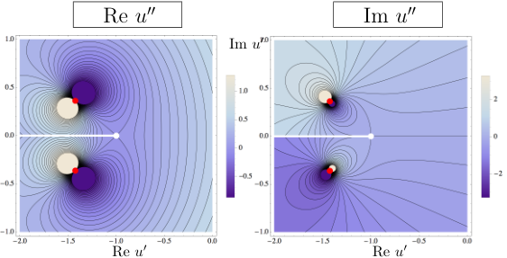
In Fig. 5, we show contour plots of $u^{\prime\prime}$ expressed in terms of $u^{\prime}$, (65), and indicate the location of the pole and the reference points $u^{\prime}=-1$ and $u^{\prime}=0$. The real part of $u^{\prime\prime}$ is $Z_{2}$-symmetric under the map Im $u^{\prime}\leftrightarrow-$Im $u^{\prime}$. In this representation we find

$$u^{\prime\prime}=\frac{1}{H^{\prime\prime}_{s}}\,\frac{1}{u^{\prime}-u^{\prime}_{s}}$$

(77)

from differentiating (73) with respect to the field. Notice that the square-root type singularity in $\rho$ (76) now becomes a simple pole in $u^{\prime}$ as it must, following (74).

Finally we turn to the regime of purely imaginary fields, corresponding to negative $\rho$. For small imaginary fields, the Taylor expansion in $\rho$ of Sec. D is applicable since the radius of convergence (52) is finite and extends to negative values. For large negative $\rho$ or large imaginary fields $\pm i\varphi\to\infty$, the effect of fluctuations is parametrically large. Furthermore, the presence of the fluctuation-induced term $\sim u^{\prime\prime}I^{\prime}[u^{\prime}]$ in the flow equation implies that $-1\leq u^{\prime}<0$. This is different from the behaviour at large positive $\rho$ where $0<u^{\prime}$ and the effects of fluctuations are suppressed, see Sec. E. We find that the fixed point solution approaches

$$u^{\prime}_{*}(\rho)\to-1$$

(78)

for asymptotically large negative $\rho$, thereby exhausting the domain of achievable values for $u^{\prime}$. Incidentally, this is also the non-perturbative fixed point of convexity, which is approached in a phase with spontaneous symmetry breaking.

Since the Wilson-Fisher fixed point solution has $u^{\prime}<0$ for field values below the VEV, it must be possible to re-cover it through an expansion about (78), which we denote as expansion $D$. The full asymptotic expansion of the Wilson-Fisher fixed point about (78) for large negative $\rho$ contains inverse powers of the fields, powers of logarithms of the field, and products thereof. The set of non-trivial operators appearing in the fixed point solution is covered by the ansatz

$$u^{\prime}(\rho)=-1+\sum_{m=1}^{\infty}\sum_{n=0}^{m-1}\zeta_{m,n}\,\left(-\rho\right)^{-m}\,\ln^{n}(-\rho)\,.$$

(79)

The structure of (79) can be understood as follows. In the limit where $u^{\prime}+1\to 0^{+}$, the first term in (21) remains non-zero, while the second term is subleading. Therefore, the first and the third term in (21) have to cancel, which is the case iff

$$0\leq 1+u^{\prime}=\frac{1}{2(-\rho)}+{\rm subleading}\,.$$

(80)

The next-to-leading term must contain a logarithm $\sim{\ln(-\rho)}/{(-\rho)^{2}}$ or else the fixed point condition cannot be satisfied. This leads to the pattern (79). Adopting our strategy, we insert the Ansatz (79) up to order $n=M$ into (23) to find $\frac{1}{2}M(M+1)$ algebraic equations for the expansion coefficients $\zeta_{m,n}$, all of which can be solved recursively in terms of a single free parameter

$$\zeta\equiv\zeta_{2,0}\,.$$

(81)

In terms of (81), the first few coefficients are explicitly given by

	$\displaystyle\zeta_{1,0}$	$\displaystyle=$	$\displaystyle\ \ \,\frac{1}{2}\,,\quad$
	$\displaystyle\zeta_{2,1}$	$\displaystyle=$	$\displaystyle\ \ \,\frac{3}{8}\,,\quad$
	$\displaystyle\zeta_{3,0}$	$\displaystyle=$	$\displaystyle-\frac{1}{32}(9+32-64\,\zeta^{2})\,,$
	$\displaystyle\zeta_{3,1}$	$\displaystyle=$	$\displaystyle\ \ \,\frac{3}{8}(4\,\zeta-1)\,,\quad$
	$\displaystyle\zeta_{3,2}$	$\displaystyle=$	$\displaystyle\ \ \,\frac{9}{32}\,,$		(82)
	$\displaystyle\zeta_{4,0}$	$\displaystyle=$	$\displaystyle-\frac{1}{512}(99-400\,\zeta-2688\,\zeta^{2}+2048\,\zeta^{3})\,,\quad\quad\quad$
	$\displaystyle\zeta_{4,1}$	$\displaystyle=$	$\displaystyle-\frac{3}{256}(25+336\,\zeta-384\,\zeta^{2})\,,$
	$\displaystyle\zeta_{4,2}$	$\displaystyle=$	$\displaystyle\ \ \,\frac{27}{256}(16\,\zeta-7)\,,$
	$\displaystyle\zeta_{4,3}$	$\displaystyle=$	$\displaystyle\ \ \,\frac{27}{128}\,,\quad$

and similarly to higher order. Using the exact result we establish

$$\zeta=\frac{3}{8}(3\ln 2-2)=0.029\,790\,578\,129\,938\,\cdots\,.$$

(83)

To estimate the radius of convergence for the expansion $D$ we adopt an iterative version of the Mercer-Roberts technique to account for the logarithms. We write the series $u^{\prime}=-1+\sum\tau_{m}(\rho)(-\rho)^{-m}$ in terms of coefficients $\tau_{m}(\rho)=\sum_{n=0}^{m-1}\zeta_{m,n}\ln^{m}(-\rho)$. Since the logarithm varies only slowly compared to powers, we approximate the coefficients $\tau_{m}=\tau_{m}(R^{(0)})$ for some trial coordinate $\rho=R^{(0)}$ to determine the radius of convergence $R^{(1)}=f(R^{(0)})$, subject to the initial guess for the radius $R_{D}=R^{(0)}$. Subsequently the intial guess is replaced by the first estimate $R_{D}=R^{(1)}$ to provide the input for the second estimate $R^{(2)}=f(R^{(1)})$ and so forth, until the procedure converges into a fixed point

$$R_{D}=f(R_{D})\,.$$

(84)

Based on the first 100 coefficients $\zeta_{m,n}$ we find a rapid convergence with

$$R_{D}=-1.51(2)\,,$$

(85)

implying that the expansion fully determines the solution in the domain

$$\frac{\rho}{\rho_{0}}\leq R_{D}\,.$$

(86)

Most importantly, the domain overlaps with both small-field expansions $A$ given in (41) and $B$, see (53). We therefore conclude that the unique Wilson-Fisher fixed point solution in the local expansion about the minimum $A$ actually fixes the entire fixed point solution globally, for all fields, with no further free parameter to be determined.

References

- [1] K. G. Wilson, Phys.Rev. B4, 3174 (1971a).
- [2] K. G. Wilson, Phys.Rev. B4, 3184 (1971b).
- [3] J. Zinn-Justin, Int. Ser. Monogr. Phys. 92, 1 (1996).
- [4] D. J. Gross and F. Wilczek, Phys.Rev.Lett. 30, 1343 (1973).
- [5] H. D. Politzer, Phys.Rev.Lett. 30, 1346 (1973).
- [6] S. Weinberg, (1979), in General Relativity: An Einstein centenary survey, ed. S. W. Hawking and W. Israel, 790- 831, Cambridge University Press, Cambridge.
- [7] D. F. Litim and F. Sannino, JHEP 12, 178 (2014), arXiv:1406.2337 [hep-th] .
- [8] A. D. Bond and D. F. Litim, (2016), arXiv:1608.00519 [hep-th] .
- [9] D. F. Litim, Phil. Trans. Roy. Soc. Lond. A369, 2759 (2011), arXiv:1102.4624 [hep-th] .
- [10] K. Wilson and J. B. Kogut, Phys.Rept. 12, 75 (1974).
- [11] J. Polchinski, Nucl.Phys. B231, 269 (1984).
- [12] C. Wetterich, Phys.Lett. B301, 90 (1993).
- [13] T. R. Morris, Int.J.Mod.Phys. A9, 2411 (1994a), arXiv:hep-ph/9308265 [hep-ph] .
- [14] D. F. Litim, Phys.Rev. D64, 105007 (2001a), arXiv:hep-th/0103195 [hep-th] .
- [15] D. F. Litim, Phys.Lett. B486, 92 (2000), arXiv:hep-th/0005245 [hep-th] .
- [16] G. R. Golner, Phys.Rev. B33, 7863 (1986).
- [17] D. F. Litim and J. M. Pawlowski, (1999), in: Krasnitz et. al. (ed.), The Exact Renormalisation Group, World Scientific, 168-185, arXiv:hep-th/9901063 [hep-th] .
- [18] J. Berges, N. Tetradis, and C. Wetterich, Phys.Rept. 363, 223 (2002), arXiv:hep-ph/0005122 [hep-ph] .
- [19] D. F. Litim and J. M. Pawlowski, JHEP 09, 049 (2002a), arXiv:hep-th/0203005 [hep-th] .
- [20] J. M. Pawlowski, D. F. Litim, S. Nedelko, and L. von Smekal, Phys. Rev. Lett. 93, 152002 (2004), arXiv:hep-th/0312324 [hep-th] .
- [21] J. P. Blaizot, R. Mendez Galain, and N. Wschebor, Phys. Lett. B632, 571 (2006), arXiv:hep-th/0503103 [hep-th] .
- [22] D. F. Litim and D. Zappala, Phys. Rev. D83, 085009 (2011), arXiv:1009.1948 [hep-th] .
- [23] A. Codello and G. D’Odorico, Phys. Rev. Lett. 110, 141601 (2013), arXiv:1210.4037 [hep-th] .
- [24] A. Codello, N. Defenu, and G. D’Odorico, Phys. Rev. D91, 105003 (2015), arXiv:1410.3308 [hep-th] .
- [25] R. Percacci and G. P. Vacca, Phys. Rev. D90, 107702 (2014), arXiv:1405.6622 [hep-th] .
- [26] P. Mati, Phys. Rev. D91, 125038 (2015), arXiv:1501.00211 [hep-th] .
- [27] A. Eichhorn, L. Janssen, and M. M. Scherer, Phys. Rev. D93, 125021 (2016), arXiv:1604.03561 [hep-th] .
- [28] K. Kamikado and T. Kanazawa, (2016), arXiv:1604.04830 [hep-th] .
- [29] A. Eichhorn, D. Mesterhzy, and M. M. Scherer, Phys. Rev. E88, 042141 (2013), arXiv:1306.2952 [cond-mat.stat-mech] .
- [30] F. Synatschke-Czerwonka, T. Fischbacher, and G. Bergner, Phys. Rev. D82, 085003 (2010), arXiv:1006.1823 [hep-th] .
- [31] D. F. Litim, M. C. Mastaler, F. Synatschke-Czerwonka, and A. Wipf, Phys.Rev. D84, 125009 (2011), arXiv:1107.3011 [hep-th] .
- [32] M. Heilmann, D. F. Litim, F. Synatschke-Czerwonka, and A. Wipf, Phys. Rev. D86, 105006 (2012), arXiv:1208.5389 [hep-th] .
- [33] D. F. Litim, Phys. Rev. Lett. 92, 201301 (2004), arXiv:hep-th/0312114 [hep-th] .
- [34] D. Benedetti and F. Caravelli, JHEP 06, 017 (2012), [Erratum: JHEP10,157(2012)], arXiv:1204.3541 [hep-th] .
- [35] M. Demmel, F. Saueressig, and O. Zanusso, JHEP 11, 131 (2012), arXiv:1208.2038 [hep-th] .
- [36] J. A. Dietz and T. R. Morris, JHEP 01, 108 (2013), arXiv:1211.0955 [hep-th] .
- [37] K. Falls, D. Litim, K. Nikolakopoulos, and C. Rahmede, (2013), arXiv:1301.4191 [hep-th] .
- [38] K. Falls, D. F. Litim, K. Nikolakopoulos, and C. Rahmede, Phys. Rev. D93, 104022 (2016a), arXiv:1410.4815 [hep-th] .
- [39] A. Margaritis, G. Odor, and A. Patkos, Z.Phys. C39, 109 (1988).
- [40] T. R. Morris, Phys. Lett. B334, 355 (1994b), arXiv:hep-th/9405190 [hep-th] .
- [41] K.-I. Aoki, K.-i. Morikawa, W. Souma, J.-i. Sumi, and H. Terao, Prog.Theor.Phys. 95, 409 (1996), arXiv:hep-ph/9612458 [hep-ph] .
- [42] K.-I. Aoki, K. Morikawa, W. Souma, J.-I. Sumi, and H. Terao, Prog.Theor.Phys. 99, 451 (1998), arXiv:hep-th/9803056 [hep-th] .
- [43] D. F. Litim, Nucl.Phys. B631, 128 (2002), arXiv:hep-th/0203006 [hep-th] .
- [44] N. Defenu, P. Mati, I. G. Marian, I. Nandori, and A. Trombettoni, JHEP 05, 141 (2015), arXiv:1410.7024 [hep-th] .
- [45] D. F. Litim, Int.J.Mod.Phys. A16, 2081 (2001b), arXiv:hep-th/0104221 [hep-th] .
- [46] D. F. Litim, JHEP 0111, 059 (2001c), arXiv:hep-th/0111159 [hep-th] .
- [47] C. Bervillier, A. Juttner, and D. F. Litim, Nucl.Phys. B783, 213 (2007), arXiv:hep-th/0701172 [hep-th] .
- [48] C. Bervillier, B. Boisseau, and H. Giacomini, Nucl.Phys. B789, 525 (2008a), arXiv:0706.0990 [hep-th] .
- [49] C. Bervillier, B. Boisseau, and H. Giacomini, Nucl.Phys. B801, 296 (2008b), arXiv:0802.1970 [hep-th] .
- [50] S. Abbasbandy and C. Bervillier, Appl.Math.Comput. 218, 2178 (2011), arXiv:1104.5073 [math-ph] .
- [51] J. A. Adams, J. Berges, S. Bornholdt, F. Freire, N. Tetradis, and C. Wetterich, Mod. Phys. Lett. A10, 2367 (1995), arXiv:hep-th/9507093 [hep-th] .
- [52] J. Borchardt and B. Knorr, Phys. Rev. D91, 105011 (2015), [Erratum: Phys. Rev.D93, 089904 (2016)], arXiv:1502.07511 [hep-th] .
- [53] J. Borchardt and B. Knorr, (2016), arXiv:1603.06726 [hep-th] .
- [54] U. Ellwanger, Z.Phys. C62, 503 (1994), arXiv:hep-ph/9308260 [hep-ph] .
- [55] D. F. Litim and J. M. Pawlowski, Phys.Rev. D65, 081701 (2002b), arXiv:hep-th/0111191 [hep-th] .
- [56] D. F. Litim and J. M. Pawlowski, Phys.Rev. D66, 025030 (2002c), arXiv:hep-th/0202188 [hep-th] .
- [57] D. F. Litim, JHEP 0507, 005 (2005), arXiv:hep-th/0503096 [hep-th] .
- [58] D. F. Litim and L. Vergara, Phys.Lett. B581, 263 (2004), arXiv:hep-th/0310101 [hep-th] .
- [59] J. Nicoll, T. Chang, and H. Stanley, Phys.Rev.Lett. 32, 1446 (1974).
- [60] D. Litim and N. Tetradis, (1995), arXiv:hep-th/9501042 [hep-th] .
- [61] N. Tetradis and D. Litim, Nucl.Phys. B464, 492 (1996).
- [62] G. N. Mercer and A. J. Roberts, SIAM J. Appl. Math. 50, 1547 (1990).
- [63] N. Tetradis and C. Wetterich, Nucl.Phys. B383, 197 (1992).
- [64] D. F. Litim, J. M. Pawlowski, and L. Vergara, (2006), arXiv:hep-th/0602140 [hep-th] .
- [65] J. Nicoll, T. Chang, and H. Stanley, Phys.Rev. B12, 458 (1975).
- [66] A. Jüttner, D. F. Litim, and E. Marchais, (2017), arXiv:1701.05168 [hep-th] .
- [67] A. Jakovac and A. Patkos, Phys. Rev. D88, 065008 (2013), arXiv:1306.2660 [hep-th] .
- [68] K. Falls, D. F. Litim, K. Nikolakopoulos, and C. Rahmede, (2016b), arXiv:1607.04962 [gr-qc] .