CERN-TH-2016-112
Physics at a 100 TeV collider: Standard Model processes
Abstract
This report summarises the properties of Standard Model processes at the 100 TeV collider. We document the production rates and typical distributions for a number of benchmark Standard Model processes, and discuss new dynamical phenomena arising at the highest energies available at this collider. We discuss the intrinsic physics interest in the measurement of these Standard Model processes, as well as their role as backgrounds for New Physics searches.
0.1 Foreword
A 100 TeV collider is under consideration, by the high-energy physics community [benedikt, cepc_website], as an important target for the future development of our field, following the completion of the LHC and High-luminosity LHC physics programmes. The physics opportunities and motivations for such an ambitious project were recently reviewed in [Arkani-Hamed:2015vfh]. The general considerations on the strengths and reach of very high energy hadron colliders have been introduced long ago in the classic pre-SSC EHLQ review [Eichten:1984eu], and a possible framework to establish the luminosity goals of such accelerator was presented recently in [Hinchliffe:2015qma].
The present document is the result of an extensive study, carried out as part of the Future Circular Collider (FCC) study towards a Conceptual Design Report, which includes separate Chapters dedicated to Standard Model physics (this paper), physics of the Higgs boson and electroweak (EW) symmetry breaking [Higgs-report], physics beyond the Standard Model [BSM-report], physics of heavy ion collisions [Dainese:2016gch] and physics with the FCC injector complex [inj-report]. Studies on the physics programme of an collider (FCC-ee) and collider (FCC-eh) at the FCC facility are proceeding in parallel, and preliminary results are documented in [Gomez-Ceballos:2013zzn] (for FCC-ee) and in [AbelleiraFernandez:2012cc] (for the LHeC precursor of FCC-eh).
0.2 Standard Model at 100 TeV: Introduction
Standard Model particles play multiple roles in the 100 TeV collider environment. In the context of BSM phenomena, and for most scenarios, new BSM particles eventually decay to the lighter SM states, which therefore provide the signatures for their production. BSM interactions, furthermore, can influence the production properties of SM particles, and the observation of SM final states can probe the existence of an underlying BSM dynamics. SM processes therefore provide both signatures and potential backgrounds for any exploration of BSM phenomena. SM backgrounds have an impact on BSM studies in different ways: on one side they dilute, and can hide, potential BSM signals; on the other, SM processes influence the trigger strategies, since they determine the irreducible contributions to trigger rates and may affect the ability to record data samples of interest to the BSM searches.
The observation of SM processes has also an interest per se. The huge rates available at 100 TeV allow, in principle, to push to new limits the exploration of rare phenomena (e.g. rare decays of top quarks or Higgs bosons), the precision in the determination of SM parameters, and the test of possible deviations from SM dynamics. The extremely high energy kinematical configurations probe the shortest distances, and provide an independent sensitivity to such deviations.
Finally, SM processes provide a necessary reference to benchmark the performance of the detectors, whether in the context of SM measurements, or in the context of background mitigation for the BSM searches.
In this Chapter we review the key properties of SM processes at 100 TeV, having in mind the above considerations. This will serve as a reference for future studies, and to stimulate new ideas on how to best exploit the immense potential of this collider. We shall focus on the production of key SM objects, such as jets, heavy quarks, gauge bosons. The SM Higgs boson will be discussed in the Higgs Chapter of this report [Higgs-report]. We shall not address issues like the current or expected precision relative to given processes. On one side, and with some well understood exceptions notwithstanding, leading-order calculations are typically sufficient to give a reliable estimate of the production rates, and assess possible implications for trigger rates, background contributions, and detector specifications. On the other, any statement about the precision of theoretical calculations made today will be totally obsolete by the time this collider will operate, and assumptions about the accuracy reach cannot but be overly conservative.
0.3 Parton distribution functions11 1 Editor: J. Rojo
0.3.1 Introduction
The accurate determination of the parton distribution functions (PDFs) of the proton is an essential ingredient of the LHC physics program [Forte:2013wc, Ball:2012wy, Rojo:2015acz, Butterworth:2015oua, Accardi:2016ndt], and will be even more so at any future higher-energy hadron collider. In particular, a new hadron collider with a center-of-mass energy of TeV will probe PDFs in several currently unexplored kinematical regions, such as the ultra low- region, , or the region of very large momentum transfers, . In addition, concerning the phenomenological implications of PDFs, the situation is much more complex (and interesting) than simply assuming that the FCC can be treated as a rescaled version of the LHC. Indeed, understanding PDFs at 100 TeV involves addressing a number of qualitatively new phenomena that have received limited attention up to now.
It is extremely difficult to forecast what the status of our knowledge about the proton structure will be in 20 or 25 years from now. Progress in PDF determinations [Ball:2014uwa, Dulat:2015mca, Harland-Lang:2014zoa, Alekhin:2013nda, Abramowicz:2015mha, Accardi:2016qay, Jimenez-Delgado:2014twa] will strongly depend, on the one hand, on the full exploitation of the information on PDF-sensitive measurements contained by LHC Run I and Run II data [Rojo:2015acz], as well as by the corresponding HL-LHC measurements, and on the other hand, on the progress in higher-order calculational techniques allowing to include many LHC differential distributions in the PDF analysis at NNLO (and beyond), see [Currie:2013dwa, Czakon:2015owf, Boughezal:2015dra] for some recent examples.
Moreover, progress in global PDF analysis can also be driven by methodological improvements, for instance in more efficient methods to parametrize PDFs, or better techniques to estimate experimental, model, and theoretical PDF uncertainties. Another important factor to take into account is the fact that our understanding of the proton structure would be substantially improved in the case a new electron-nucleon collider would be operative before the start-up of the FCC operations, such as the Large Hadron Electron Collider (LHeC) at CERN [AbelleiraFernandez:2012cc] or the Electron Ion Collider (EIC) in the U.S.A. [Boer:2011fh]. In addition, in the long term, progress in non-perturbative lattice calculations might also shed further light on the proton structure and provide a useful complement to global PDF fits.
For these reasons, in this section we will concentrate on qualitative aspects of PDFs that are important for a exploratory evaluation of the physics potential of the FCC, which is the main goal of this report. In particular we will focus on:
- •
What are the most relevant generic differences for PDFs when moving from the LHC energies, 14 TeV, to the FCC energies, 100 TeV.
This includes the kinematical coverage in the plane of a 100 TeV collider, the ratios of PDF luminosities and their uncertainties between 100 TeV and 14 TeV, and the assessment of how available PDF sets extrapolate into the new kinematical regions covered by the FCC.
- •
Qualitatively new phenomena about PDFs and DGLAP evolution that, while not essential for the exploitation of the LHC data, might become relevant at the extreme energies at which the FCC would operate.
These include QED and weak effects in the PDF evolution, high-energy resummation effects, and the possibility of treating the top quark as a massless parton. In addition, we also study the role of photon-initiated contributions for electroweak processes at 100 TeV.
The outline of this section is the following. In Sect. 0.3.2 we quantify the coverage of PDFs at the FCC in the plane, and study the behavior of PDFs in the extreme large-, large- and small- regions accessible at the FCC. In Sect. 0.3.3 we present a comparison of PDF luminosities at 100 TeV for the most updated global PDF sets, and compute various ratios of parton luminosities between 100 TeV and 14 TeV. In Sect. 0.3.4 we study the validity of the massless approximation for the top quark at a 100 TeV collider. In Sect. 0.3.5 we quantify the role of photon and lepton-initiated contributions at 100 TeV, relevant when electroweak corrections are accounted for. In Sect. 0.3.6 we explore the possibility of treating electroweak gauge bosons as massless and their inclusion into the DGLAP evolution equations. Finally in Sect. 0.3.7 we discuss the possible relevance of high-energy (small-) resummation effects for a 100 TeV collider.
0.3.2 PDFs and their kinematical coverage at 100 TeV
We begin by quantifying the kinematical coverage in the plane that PDFs probe in a 100 TeV hadron collider, with being the invariant mass of the produced final states. In Fig. 1 we represent the kinematical coverage in the plane of a TeV hadron collider compared with the corresponding coverage of the LHC at TeV. The dotted lines indicate regions of constant rapidity at the FCC. In this plot, we also indicate the relevant regions for phenomenologically important processes, from low masses (such as Drell-Yan or low jets), electroweak scale processes (such as Higgs, , or top production), and possible new high-mass particles (such as a 2 TeV squark or a 20 TeV ).
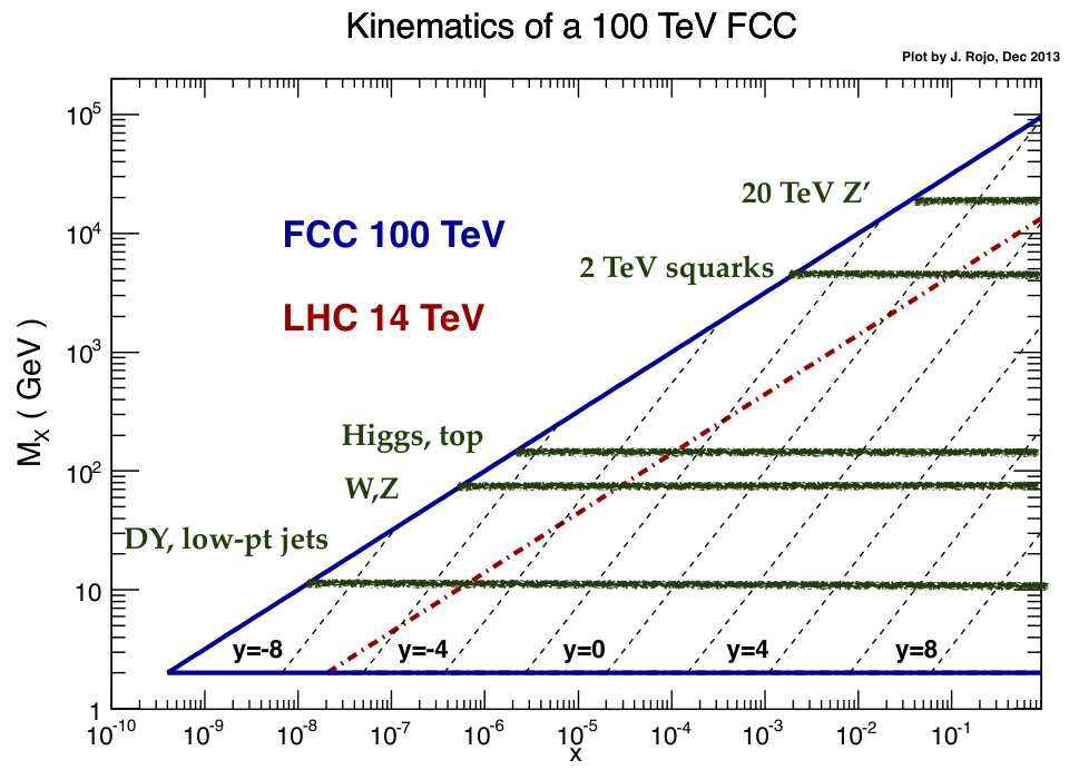
In the low-mass region, for GeV, PDFs would be probed down to in the central region, , and down to at forward rapidities, . At even forward rapidities, for example those that can be probed by using dedicated detectors down the beam pipe, PDFs could be probed down to . While these extreme regions of very low are not relevant for neither electroweak scale physics nor for high-mass New Physics searches, they are crucial for the tuning of soft and semi-hard physics in Monte Carlo event generators [Skands:2014pea] and therefore it is important to ensure that the PDFs exhibit a sensible behaviour in this region. Moreover, forward instrumentation would also be relevant for the measurement of the total cross-section at 100 TeV as well as to provide input for the modelling of ultra-high energy cosmic ray collisions [d'Enterria:2011kw]. The prospects for soft physics at the FCC is studied in detail in Sect. 0.4 of this report.
Concerning the production of electroweak particles such as weak gauge bosons, the Higgs boson and top quarks, PDFs are probed down to in the central region, , and down to at forward rapidities, . This indicates that a good coverage of the forward region is also instrumental for electroweak scale physics, whose production is much less central than at the LHC. In the case of Higgs production, if the Higgs can be reconstructed up to rapidities of , then this process would probe PDFs down to . Therefore, at a 100 TeV hadron collider a good knowledge of small- PDFs becomes crucial not only for soft and semi-hard physics, or for low scale processes such as low-mass Drell-Yan or charm production, but also for electroweak scale processes.
In the high-invariant mass region, TeV, only medium and large- PDFs would be probed, and these are currently known with reasonable accuracy, except for very high values. For instance, for the pair-production of 2 TeV squarks, only the knowledge of PDFs for is required. The production of multi-TeV heavy particles is of course very central, requiring instrumentation only down to at most. For the heavier particles that can be probed at the FCC, such as a 20 or 30 TeV , PDFs have large uncertainties since the very large- region is being probed, and this region is affected by the lack of direct constraints, as we discuss below.
In Table 1 we summarize the kinematical coverage in the plane for various phenomenologically important processes at the FCC, both for central, intermediate and forward rapidities. For each value of the invariant mass and the absolute rapidity , the smallest value of Bjorken- required corresponds to . This table conveys a similar message to that of Fig. 1: at a 100 TeV hadron collider, accurate knowledge of PDFs is required in a very wide kinematical region, ranging from ultra low- to very large-, and from momentum transfers close to up to the highest values where the FCC has sensitivity for new heavy particles, TeV. That is, a huge range spanning 8 orders of magnitude in and 10 in .
| Process | ||||
| Soft QCD | 1 (10) GeV | |||
| Charm pair production | ||||
| Low-mass Drell-Yan | ||||
| and production | 80 (400) GeV | |||
| Top pair production | ||||
| Inclusive Higgs | ||||
| Heavy New Physics | 5 (25) TeV | 0.05 (0.25) | 0.007 (-) | – |
Given this, it is important to verify that available PDF sets have a sensible behaviour in all the relevant kinematical regions, specially in the extrapolation regions at very small- and very large which are not relevant for most LHC applications. The goal here is not to understand similarities or differences between PDF sets, but to ensure that PDF sets that will be used for FCC simulations have a physical behaviour in the entire range of and required.
In the following, PDFs are accessed through the LHAPDF6 interface [Buckley:2014ana], version 6.1.5, with the most updated grid data files. It should be emphasized the importance of using this specific version, since previous versions had different options for the default PDF extrapolations. In addition, both the interpolation accuracy and the treatment of the extrapolation regions, as well as the overall computational performance, have been substantially improved in LHAPDF6 as compared to its Fortran counterpart LHAPDF5, and therefore the use of the latter for FCC studies should be discouraged.33 3 In LHAPDF5 the default extrapolation was simply to freeze the PDF below some value of , which could be as high as for some widely used PDF sets, which can potentially lead to incorrect results if used for FCC studies.
We begin by discussing the PDF behavior in the small- extrapolation region. As shown in Fig. 1, for low scales and forward rapidities, as those required for the description of soft QCD physics and for Monte Carlo tuning, knowledge of PDFs would be required down to . In Fig. 2 we show the central values of the gluon (upper) and the up quark PDFs (lower plots), comparing ABM12, CT14, MMHT14 and NNPDF3.0 for GeV2. All PDF sets shown are NLO except for ABM12 where the NNLO set is used. The comparison is performed down to , to ensure that the entire region relevant for FCC studies is covered. In all cases we observe a sensible extrapolation into the very small- region. Here we use the default extrapolating settings of LHAPDF6.1.5, and we verified that the behaviour was instead unphysical if older versions were used, where PDFs were frozen for some threshold.
While in Fig. 2 we only show the central values of the three PDF sets, in the small- region these are affected by substantial uncertainties [Gauld:2015yia] due to the lack of direct experimental constraints, for instance, the HERA structure functions data stops at , see for instance the measurement of the longitudinal structure function [Collaboration:2010ry, Abramowicz:2015mha]. To illustrate this point, in Fig. 3 we show the relative 68% CL PDF uncertainties at GeV2 in the small- region for the ABM12, CT14, MMHT14 and NNPDF3.0 NNLO sets. Depending on the model chosen to parametrize PDF uncertainties towards the region without experimental constraints, we observe a rapid increase in PDF uncertainties for some sets (CT14, MMHT, NNPDF3.0), where for uncertainties are already larger than 50%, while other sets (ABM12, but also CJ15, JR14 not shown here) display small PDF uncertainties down to .
Recently, a number LHC measurements to constrain PDFs at small- has been proposed. The use of charmed meson forward production from LHCb has been recently shown [Gauld:2015yia, Cacciari:2015fta, Zenaiev:2015rfa] to provide useful constraints on the small- gluon PDF.44 4 The PDF dependence of heavy quark production at a 100 TeV collider is discussed in more detail in Sect. 0.12 of this report. Another possibility is the use of forward quarkonium production, such as , which has a similar sensitivity in [Jones:2015nna]. Taking this into account, one expects that before the FCC start-up our knowledge of the small- PDFs would be substantially improved. The corresponding measurements at the FCC have the potential to extend the constrains on the small- PDF by almost two orders of magnitude, though here the instrumentation of the forward region will be crucial. Measurements of very-small- PDFs are also of direct importance for particle astrophysics, such as the ultra-high-energy neutrino cross-sections [CooperSarkar:2011pa] and the prompt lepton fluxes [Gauld:2015kvh, Bhattacharya:2015jpa, Garzelli:2015psa] that are required for the interpretation of the IceCube astrophysical neutrinos [Aartsen:2014gkd].
Another strategy to quantify the relevant range of Bjorken- for which PDFs are required in the modeling of soft and semi-hard physics at the FCC is by sampling of the values of of the PDFs required in the calculation of Multiple Parton Interactions (MPI) for different values of the collider center-of-mass energy . In Fig. 4 we compare the MPI sampling of between the LHC 7 TeV and the FCC 100 TeV using Pythia8.2 [Sjostrand:2014zea]. The results of the most update tune, Monash 2013 [Skands:2014pea] are compared with the older tunes 2C and 4C [Skands:2010ak]. From this comparison we observe that, with the Monash 2013 tune, at LHC7, PDFs with lead to a sizable contribution, , to the MPI distribution. With the same settings, the FCC100 samples values of down to , a region far from any direct experimental constraint. This illustrates the relevance of ultra-low PDFs for the modelling of soft QCD at a 100 TeV collider.
Now we turn to discuss the region of large values of Bjorken-. This region is also affected by substantial PDF uncertainties due to the limited direct experimental constraints. To estimate the coverage in the large- region, it is useful to use the result that for the production of a final state with invariant mass and rapidity at a hadron collider with center-of-mass energy , the LO values of the PDF momentum fractions and are . Therefore, for a centrally produced final-state () of invariant mass TeV (50 TeV) at 14 TeV (100 TeV) we will have , while already for slightly non-central production, , PDFs are being probed up to for both colliders.
In Fig. 5 we illustrate the large- behaviour of the up, down, anti-up quark and gluon PDFs, evaluated at GeV. We compare the results of the ABM12, CT14, NNPDF3.0 and MMHT14 NNLO PDF sets, with the corresponding 68% CL PDF uncertainty in each case, normalising to the central value of CT14.55 5 In these plots, the ABM12 curves have been obtained using the internal interpolation routine provided by the authors, since the LHAPDF6 results were found to exhibit poor numerical stability at large . As discussed above, the central production of a heavy system with TeV would probe the large- PDFs for (0.3 or 0.5) at a 100 TeV collider. As we can see, while for valence quarks (up and down) PDF uncertainties in the region relevant for heavy particle production at the FCC are moderate, for the gluon and anti-quarks PDF uncertainties are large, thus degrading the accuracy of any theory prediction that requires knowledge of PDFs in this region. In addition, there is a significant spread between the central values of the four sets.
As in the case of small-, new measurements from the LHC and other experiments should allow to substantially reduce these PDF uncertainties before the start of FCC operations. For instance, the large- gluon can be constrained with data on inclusive and differential top quark pair production [Czakon:2013tha, Guzzi:2014wia]. Moreover, since at large- and large- the gluon and sea quark distributions receive large contributions from radiation off valence quarks, measurements aiming to constrain these will also lead to improved gluons and sea quarks in the kinematic region relevant for the FCC. This effect is illustrated in Fig. 6, where we show the ratio of parton distributions, with respect to the initial parametrization for the gluon and sea distributions at large . The solid line denotes the initial PDF suppressed by a factor of for the gluon (left panel) and up quarks (right panel) and the dotted and dashed-dotted lines the respective results of the evolution up to = 20 TeV. One should also note that, as in the case of small-, the behaviour of PDFs in the large- extrapolation region is sensitive to the underlying assumptions concerning the PDF parametrization [Ball:2016spl].
PDFs at large- are also affected by a number of theoretical uncertainties, from potential higher twists, enhanced higher-order threshold logarithmic corrections, or nuclear effects from the inclusion in the PDF fit of deuteron and heavy nuclear data. A version of NNPDF3.0 including large- threshold resummation was presented in [Bonvini:2015ira], and then used [Beenakker:2015rna] to produce threshold-improved NLO+NLL predictions for high-mass squark and gluino production cross-sections at the LHC. This study showed that threshold logarithms in PDF fits are much smaller than PDF uncertainties, provided NNLO calculations are used. Therefore, PDFs with threshold resummation do not appear to be required for FCC studies, since NNLO and N3LO calculations will be the standard by then. Likewise, other theory uncertainties like higher twists and nuclear effects are subleading as compared to PDF uncertainties (see the discussion in [Ball:2013gsa, Butterworth:2015oua] and references therein), and moreover by the time the FCC starts operation, reliable collider-only PDF sets, free of these ambiguities, will be available.
The other kinematic region for which knowledge of PDFs will be required in a previously unexplored region is that of very large momentum transfers, for values of between 5 TeV and 50 TeV. This region is relevant for the production of possible massive BSM particles. As opposed to the small- and large- regions, the extrapolation into very high values is determined purely by perturbative DGLAP evolution, and therefore the only requirement is that that available PDF tabulations of current sets extend up to 100 TeV. We have verified that this is the case for the modern PDF sets discussed in this chapter. However, the argument above however holds only for QCD evolution. It should be taken into account that differences in the upwards evolution in can arise if the evolution equations are modified, for instance in the case of electroweak corrections to DGLAP evolution, Sect. 0.3.6, or in the presence of high-energy resummation effects, Sect. 0.3.7.
In Fig. 7 we compare, for , the evolution of the central values of the gluon and up quark PDFs for the NNPDF3.0, CT14 and MMHT14 NNLO sets, from a very low scale, GeV, up to the highest possible scales that the FCC can reach, TeV. It can be verified, by comparing with public PDF evolution packages such as HOPPET [Salam:2008qg] or APFEL [Bertone:2013vaa], that the tabulated extrapolation up to very high of modern PDF sets is consistent with DGLAP evolution as expected.66 6 Again, this is not necessarily true for older PDF sets. In some cases the coverage in was restricted to 10 TeV, and from there upwards an unphysical (non-DGLAP) extrapolation was used. As in the case of large and small-, use of these older sets can lead to incorrect results in the context of FCC simulations. We conclude that, provided modern PDF sets are used, the extrapolation of the DGLAP evolution in to the region relevant at the FCC is reliable.
0.3.3 PDF luminosities at 100 TeV
Parton luminosities are useful to estimate the PDF dependence of hadron collider cross-sections, by taking into account the most relevant initial-state production channels. While several definitions of the PDF luminosity can be adopted, in the following we will use the luminosities as a function of the invariant mass of the produced final state, , defined as
| (1) |
where and are PDF flavour indices, , and is the collider center-of-mass energy. Another useful way of representing PDF luminosities is as two-dimensional functions of rapidity and invariant mass of the final state,
| (2) |
which leads to Eq. (1) upon integration over the kinematically allowed range for the rapidity , that is,
| (3) |
Typically PDF luminosities are presented summing over quark flavor indices, and here we adopt the following convention:
| (4) | |||||
for the luminosities integrated in rapidity Eq. (1), and similar definitions for the double differential luminosities Eq. (2). Eq. (4) can be trivially generalized to the case in which the top quark is treated as a massless parton.
In Fig. 8 we show the rapidity-integrated PDF luminosities Eq. (1), as a function of the invariant mass of the system , for the PDF4LHC15_nnlo_mc PDF set [Butterworth:2015oua, Carrazza:2015hva], with PDF uncertainties computed at 68% confidence levels.
We show the gluon-gluon, quark-gluon, quark-quark and quark-antiquark luminosities, normalized to the corresponding central value, for the case of a TeV collider. Similar comparisons in the case of the LHC 14 TeV can be found in [Butterworth:2015oua]. We find PDF uncertainties are at the 5% level for TeV for all four PDF luminosities. They become more important at larger values of , relevant for heavy particle searches, and for smaller values of , relevant for electroweak physics and semi-hard QCD. For instance, at TeV the gluon-gluon PDF luminosity has an associated uncertainty of around 20%. For the production of electroweak scale particles PDF uncertainties are increased when going from the LHC to the FCC, due to the smaller values of probed in the latter case. For GeV, relevant for inclusive Higgs and weak gauge boson production, PDF uncertainties are around the 10% level. It can also be instructive to plot the absolute PDF luminosities in each channel together with the corresponding PDF uncertainties, this is done in Sect. 0.3.5 later in this chapter.
We now turn to discuss the double-differential PDF luminosities, Eq. (2), evaluated for a center of mass energy TeV. In Fig. 9 shows the PDF uncertainties, evaluated as 68% CL, on the luminosities as a function of and of the rapidity . As above, the PDF4LHC15_nnlo_mc PDF set is used as input. Fig. 9 represents the contours of constant PDF uncertainties in the different flavour combinations. One sees that for all flavour combinations, the uncertainties are smallest, of the order of , for pair invariant masses of the order of a TeV. They also all have a characteristic dip at rapidities of about . One may speculate that this is a consequence of an anti-correlation between moderately large and small- parton distributions caused by momentum conservation. For partonic-pair masses at the electroweak scale and in the region above a few TeV, uncertainties grow larger. In all cases PDF uncertainties grow large near the kinematic boundaries, since these are sensitive to to PDFs at small and large- that currently are constrained by few experimental measurements.
Next we compute the ratio of the rapidity-integrated PDF luminosities between 100 TeV and 14 TeV, for different initial-state partonic channels, defined as:
| (5) |
with TeV and TeV. Such ratios provide a convenient rule of thumb to rescale production cross-sections between 14 and 100 TeV, for processes dominated by a single initial-state luminosity. Eq. (5) can thus be used to estimate ratios of cross-sections between the different center-of-mass energies. These cross-section ratios, in addition to providing stringent SM tests and potential PDF-constraining information, could also be used as an alternative method to search for new physics at the FCC [Mangano:2012mh].
In Fig. 10 we show the ratio of PDF luminosities, Eq. (5), between the FCC TeV and the LHC TeV, for the four different initial-state channels. These ratios have been computed with both the NNPDF3.0 and the PDF4LHC15_nnlo_mc NNLO sets, to illustrate that the generically depends only very mildly of the specific input PDF set used. In Fig. 10 we also include the 68% CL PDF uncertainties in the luminosity ratio, accounting for the correlations between the results at the two values of the center-of-mass energy. The ratio is computed between GeV and TeV, the highest invariant masses that the LHC can reach. From this comparison, we observe that for low invariant masses, GeV, the increase in parton luminosities when going from the LHC to the FCC is moderate, a factor 10 at most. In this region the luminosity ratio is affected by large PDF uncertainties, arising from the production of a small final state at the FCC, which probes small- PDF.
On the other hand, the luminosity ratio increases rapidly as we move away from the electroweak scale, since these the increase in energy of the FCC dramatically dominates over the large- fall-off of the PDFs at the LHC. For invariant masses around TeV, for instance, the , , and luminosity ratios are and 10, respectively. Gluon-initiated processes are those that benefit more from the increase in center-of-mass energy due to the rapid rise of the gluon PDF at medium- and small- from DGLAP evolution. For the highest invariant masses that can be probed at the LHC, TeV, the values of the ratios (in the same order) are , , and 200. The hierarchy is maintained for all invariant masses above GeV.
The results in Fig. 10 can be used to compare with the various ratios of cross-sections between 100 TeV and 14 TeV collected elsewhere in this report. In order to facilitate the comparison with ratios of cross-sections between different center-of-mass energies presented elsewhere in this report, in Table 2 we provide the corresponding numerical values of the PDF luminosity ratios show in Fig. 10 for the case of the PDF4LHC15_nnlo_mc PDF set.
| (GeV) | ||||
|---|---|---|---|---|
| 50 | 8.8 0.3 | 6.9 0.3 | 5.7 0.4 | 5.9 0.4 |
| 58 | 9.5 0.3 | 7.4 0.3 | 5.9 0.4 | 6.3 0.4 |
| 68 | 10.3 0.3 | 7.9 0.3 | 6.3 0.3 | 6.6 0.3 |
| 80 | 11.2 0.3 | 8.5 0.3 | 6.6 0.3 | 7.0 0.3 |
| 94 | 12.2 0.3 | 9.1 0.2 | 7.0 0.2 | 7.3 0.2 |
| 111 | 13.4 0.3 | 9.7 0.2 | 7.4 0.2 | 7.8 0.2 |
| 130 | 14.7 0.3 | 10.5 0.2 | 7.8 0.2 | 8.2 0.2 |
| 152 | 16.2 0.4 | 11.3 0.2 | 8.2 0.2 | 8.7 0.2 |
| 178 | 18.0 0.4 | 12.2 0.2 | 8.7 0.2 | 9.2 0.2 |
| 209 | 20.0 0.4 | 13.3 0.2 | 9.2 0.2 | 9.8 0.2 |
| 245 | 22.5 0.4 | 14.5 0.2 | 9.8 0.2 | 10.5 0.2 |
| 287 | 25.4 0.5 | 15.8 0.2 | 10.5 0.2 | 11.3 0.2 |
| 336 | 28.9 0.6 | 17.4 0.2 | 11.1 0.2 | 11.9 0.3 |
| 394 | 33.2 0.8 | 19.3 0.3 | 12.0 0.2 | 13.0 0.2 |
| 462 | 38.6 0.9 | 21.5 0.3 | 13.0 0.2 | 14.0 0.2 |
| 541 | 45.1 1.2 | 24.2 0.3 | 14.1 0.2 | 15.2 0.2 |
| 634 | 54.0 1.6 | 27.4 0.4 | 15.4 0.3 | 16.5 0.2 |
| 744 | 65.3 2.2 | 31.4 0.5 | 17.0 0.3 | 18.1 0.2 |
| 872 | 80.8 2.8 | 36.4 0.6 | 19.0 0.4 | 19.9 0.3 |
| 1022 | 101 4 | 42.9 0.7 | 21.6 0.5 | 22.0 0.3 |
| 1198 | 131 6 | 51.6 1.0 | 25.1 0.6 | 24.7 0.3 |
| 1403 | 173 9 | 63.5 1.4 | 29.9 0.8 | 27.9 0.4 |
| 1646 | 238 14 | 80.3 1.8 | 37.0 1.1 | 32.5 0.7 |
| 1928 | 341 25 | 105 3 | 47.6 1.8 | 37.7 0.6 |
| 2260 | 517 45 | 143 5 | 65.0 2.9 | 45.4 0.7 |
| 2649 | 837 90 | 207 9 | 94.7 4.9 | 56.7 1.0 |
| 3105 | 1454 200 | 322 15 | 151 9 | 74.8 1.4 |
| 3639 | 2815 512 | 546 33 | 269 18 | 106 2 |
| 4265 | 6233 1395 | 1047 84 | 549 50 | 168 5 |
| 5000 | 16646 4557 | 2356 249 | 1366 207 | 308 10 |
0.3.4 The top quark as a massless parton
At a 100 TeV hadron collider, particles with masses around the electroweak scale appear as comparably light as the bottom quark at the Tevatron collision energy of . When a very heavy scale is involved in the process, the gluon splitting into a top-antitop pair may present a large logarithmic enhancement. For , for instance, , which makes a perturbative expansion of the hard process questionable. Therefore, one might wonder if the concept of top quark PDF is relevant at the FCC, just as charm and bottom PDFs are commonly used in LHC calculations. The question is then what is more suitable and advantageous, from a calculational point of view, to use at the FCC: a fixed-flavor number (FFN) scheme, where the top is a massive quark, or a variable-flavor number (VFN) scheme, where the top is a massless parton? The discussion is thus completely analogous to the case of bottom quarks at the LHC [Maltoni:2012pa].
As with the charm and bottom quarks, introducing a PDF for the top quark inside the proton allows us to resum potentially large collinear logarithms of the form to all orders in perturbation theory. The generalization of the DGLAP evolution equations to include a top PDF up to NNLO is straightforward, and indeed most modern PDF sets provide variants where the maximum number of light quarks in the PDF evolution is set to . Indeed, the majority PDF fits are performed in a VFN scheme with a maximum of light partons, since in the fitted hard cross-sections top is always treated as a massive quark, and the resulting PDFs at can then be used as boundary condition to construct the PDFs including a top quark.
In Fig. 11 we show the top quark PDF, evaluated at TeV, compared with the other light partons, in the case of the NNPDF2.3NNLO PDF set [Ball:2012cx]. We observe that the top quark PDF can be of a similar size as the light quark PDFs, in particular at medium and small-, the region where the effects of DGLAP evolution are dominant. We also see that the charm and bottom PDFs are essentially indistinguishable from the light quark PDFs for . In Fig. 11 we also show the ratio between the gluon PDF between the and schemes, as a function of the factorization scale . We observe that the differences between the two schemes can be up to several percent for TeV, a region well covered by the FCC kinematics. Therefore, the use of the scheme would also have implications for precision calculations involving gluons and light quarks, and not only those with initial state top quarks.

So while technically generating a top quark PDF is straightforward, it still needs to be determined if it provides any calculational advantage over using the standard FFN scheme approach, where the top quark is always treated as massive, even for the extreme energies of a 100 TeV collider. This issue has been recently studied in [Han:2014nja, Dawson:2014pea], both reaching similar conclusions: a purely massless treatment of top quarks is unreliable even at the FCC, but the concept of a top quark PDFs is certainly relevant in the context of matched calculations. To illustrate this point, in the left plot of Fig. 12, taken from [Han:2014nja], we show a comparison of calculations in the 5-flavor, massless 6-flavor, and ACOT matched[Aivazis:1993pi, Collins:1998rz] schemes for the inclusive production of a hypothetic heavy scalar, labeled , at a TeV proton-proton collider. This calculation uses as input the NNPDF2.3NLO set [Ball:2012cx]. The ACOT scheme shows the desired behavior of interpolating between the region near the top threshold and the very high energy limit (where collinear logarithms in the top quark mass become large). It should be stressed that the simplest LO calculation is unreliable even for masses as large as TeV, indicating that the minimum scale above which a parton interpretation for the top quark becomes justified is much larger than the top mass itself.
The fact that the massless approximation for top production works rather worse than for charm and bottom quarks can be traced back, at least partially, to the fact that the resummed collinear logarithms are substantially smaller as compared to the other heavy quarks. This is illustrated by the right plot in Fig. 12, taken from [Dawson:2014pea], which compares the size of the collinear logarithm as a function of the ratio for the three heavy quarks: charm, bottom and top. Even for very large ratios , the need for resummation of collinear logarithms in the top quark mass is not evident, since , while being large, is perturbative in the relevant kinematical range. This is opposed to charm, and to a lesser extend bottom, whose corresponding logarithms eventually become non-perturbative and require collinear resummation. One reason that partially explains this difference is the fact that , which allows a much larger lever arm in before resummation is required.

So in conclusion, current studies indicate, while the purely massless approximation for top quarks is unreliable even at the extreme FCC energies, the concept of top quark PDF is certainly useful in order to construct matched calculations. This way, one can supplement and improve massive fixed-order calculations with all-order resummations of collinear logarithms in matched schemes such as ACOT [Aivazis:1993pi, Collins:1998rz] or FONLL [Cacciari:1998it, Forte:2010ta]. For example, as shown in the heavy quark chapter of this report, Sect. 0.12, it is possible to generalize the FONLL calculation for the distribution in for heavy flavor differential distributions [Cacciari:1998it] to the case of top quark production at the FCC. The matched calculation is found to provide a more precise estimate in the region of transverse momenta up to 10 TeV. Eventually, this matching can be performed up to NNLO order, using the corresponding calculations for jet production [Currie:2013dwa] and for top quark production [Czakon:2015owf].
0.3.5 Photon- and lepton-initiated processes at 100 TeV
A 100 TeV Future Circular Collider is bound to probe the interactions of elementary particles at extreme energies with high accuracy. In order to correctly identify possible BSM effects, the theoretical predictions for the SM processes have to match the precision of the corresponding experimental measurements. In other words, the impact of higher-order corrections on phenomenological predictions has to be under control. To this purpose, the computation of NLO QCD corrections is necessary, but often not sufficient. In fact, at fixed order the inclusion of the NNLO QCD corrections in QCD as well as of the EW corrections is in general desirable and in particular cases even essential. The implications of higher-order EW corrections to matrix elements for FCC processes is discussed elsewhere in this report.
In order to formally achieve the desired level of accuracy, not only the matrix elements of the hard processes, but also the parton distribution functions (PDFs) of the proton, have to be known at the same level of precision. While most PDF groups provide since some time PDF sets accurate up to NNLO in QCD [Ball:2014uwa, Harland-Lang:2014zoa, Dulat:2015mca, Abramowicz:2015mha, Alekhin:2013nda], for EW corrections the situation is less satisfactory. Indeed, EW corrections require the calculation of photon-induced processes, and thus PDFs both with QED effects in the evolution and with a determination of the photon PDF are necessary for consistent calculations. In this respect, a number of PDF sets with a photon PDF and QED effects are available in LHAPDF: MRST2004QED [Martin:2004dh], NNPDF2.3QED [Ball:2013hta] and the recent CT14QED [Schmidt:2015zda]. In addition, PDF evolution with QED effects has been implemented in the APFEL PDF evolution program [Carrazza:2014gfa, Bertone:2013vaa] at LL, and inclusion of NLL QED splitting functions [deFlorian:2015ujt] is underway.
The determination of the photon PDF obtained by the three groups differ in a number of important aspects. First, different data sets are used in the fits. Second, the form of the photon distribution at the initial scale is different. Finally, the DGLAP evolution from to the final scale is not the same in all cases. As far as the functional form of the PDF at the initial scale is concerned, NNPDF2.3QED only assumes that the photon PDF is positive-definite. In a first step, PDF replicas for all partons are fitted to deep-inelastic structure functions, which only provide very loose constraints on the photon PDF. In a second step, the photon PDF is constrained from LHC Drell-Yan data. This constraint enters at LO, however, because the photon-initiated component of Drell-Yan production is small, even the relatively precise LHC data constrain the photon PDF only weakly. In particular, since no data is available at large and no functional form is assumed, in this region PDF uncertainties on turn out to be quite large.77 7 High-statistics Drell-Yan measurements at the LHC such as the recent ATLAS 8 TeV high-mass analysis [Aad:2016zzw] should provide additional information in this region.
In contrast to the NNPDF2.3QED determination, the CT14QED and MRST2004QED sets are based on the assumption that the functional form of the photon PDF at the initial scale can be determined by the valence-quark distributions. In essence, they are given by a convolution of valence-quark distributions with the splitting functions, with a normalization for the up- and down-type distributions that differ in the two approaches. Determining the photon PDF reduces then to fixing one or two parameters in the CT14QED and MRST2004QED approaches, respectively. For the CT14QED, set the constraints are obtained by fitting ZEUS data for the production of isolated photons in DIS, while for MRST2004QED an assumption is made for the normalization coefficients and no data are used to constraint the photon PDF.
Recently the CT collaboration also released a photon PDF that includes the elastic component of the photon PDF (CT14QEDinc) obtained in the so-called photon equivalent approximation, which involves an integration over the proton electromagnetic form factors. In fact, the photon PDF, unlike the quark and gluon PDFs, has a large elastic component in which the proton remains intact (see [Martin:2014nqa, Harland-Lang:2016apc, Harland-Lang:2016lhw] and references therein). This component has not been discussed in the NNPDF2.3QED and MRST2004QED fits, but is included in the photon PDF determination of [Harland-Lang:2016apc]. Another important difference is connected to the DGLAP evolution: in the evolution of the CT14QED and MRST2004QED the scale is evolved simultaneously for the QCD and for the QED evolution, while in the NNPDF2.3QED approach the two scales run independently. Very recently, in Ref. [Bertone:2016ume], the NNPDF3.0QED set has been derived, which combines the NNPDF3.0 quark and gluon PDFs with the NNPDF2.3 photon PDF using the same solution of the DGLAP equations as CT14QED and MRST2004QED.
All these differences result in predictions for the photon PDF from different sets that are not always compatible. In particular, as compared to NNPDF2.3QED, the CT14QED and MRST2004QED photon distribution functions are softer at large , and exhibit smaller PDF uncertainties due to their more restrictive parametrizations. It will be important to understand and resolve the sources of these differences between QED PDF sets. In the following we will present results based on the NNPDF2.3QED set, with the caveat that conclusions could be rather different if other QED sets were used as input to the calculations.
At very high energies, even PDFs for electroweak massive gauge bosons might be required, and this possibility is discussed in Sect. 0.3.6 below. On top of the photon-induced processes, higher-order EW corrections also induce lepton-initiated channels whose computation formally requires the knowledge of the leptonic content of the proton [Bertone:2015lqa]. To determine the lepton PDFs, the first step is to include them in the DGLAP evolution equations with QED corrections [Bertone:2015lqa], which mixes the evolution of the lepton and photon PDFs with that of quarks and gluons. Next one needs to adopt suitable boundary conditions , the initial scale lepton PDFs. Since a determination of lepton PDFs from data is hardly achievable because of their smallness, here we assume that the light lepton PDFs, , electrons and muons, are purely generated by photon splitting at the respective mass scales.
Under this assumption, one can approximate their distributions at the initial scale GeV as:
| (6) |
with the QED running coupling constant. The lepton PDFs are then dynamically generated from threshold using the standard variable-flavour-number scheme [Forte:2010ta, Aivazis:1993pi, Thorne:1997ga]. Here we will use use the apfel_nn23qednlo0118_lept set of PDFs [Bertone:2015lqa] generated starting from the NNPDF2.3QED NLO set using the Ansatz in Eq. (6) for the light lepton PDFs.
Before studying the size of photon- and lepton-initiated processes at a 100 TeV collider, it is useful to study the behaviour of the parton luminosities of the different initial states, by including also photon and leptons initiated processes. Parton luminosities can either be defined as a function of , the invariant mass of the final state, as done in Eqns. (1)–(4), or in terms of , the rapidity of the final state, integrating over the invariant mass,
| (7) |
with . In Eq. (7) the lower bound of the integral, proportional to , implies that .
In Fig. 13 we compare the size and the shape of the different parton luminosities for an hadron collider with a center of mass energy TeV, both as a function of the invariant mass (left plot) and of the final-state system rapidity (right plot). For the rapidity-dependent luminosities, we impose a cut of GeV. In Figs. 13 we also plot the corresponding 68% confidence level PDF uncertainties for each luminosity type, separating the luminosities involving photon or lepton PDFs (central panel) and those involving only quarks or gluons (lower panel). The central value of the luminosities is assigned to be the midpoint of the 68% confidence level interval, and thus by construction PDF uncertainties will not exceed 100%, as can be seen in the central panel of Fig. 13 (left).
The relative size of the plotted luminosities follows the expected pattern. In general, the photon PDF suppresses the luminosity by a factor of with respect to the (anti)quark PDFs and, analogously, the lepton PDFs suppress the luminosity by an additional factor of with respect to the photon PDF. This can be easily seen in Fig. 13, e.g. by comparing () with () and (), the three lowest curves. However, from Fig. 13 we also notice that this hierarchy is not satisfied at large invariant masses. In this kinematic region, large , one is probing PDFs at rather large values of , and here the pure-QCD luminosity combinations, , and , become closer to the luminosities involving photons and leptons, with important phenomenological implications: as opposed to the naive expectation, photon- and lepton-initiated contributions can become as large as the standard quark-initiated contributions. However, it is important to keep in mind that the uncertainty in the NNPDF2.3QED luminosity determinations involving photons (shown in the middle panel of Fig. 13) is very large, and that the NNPDF2.3QED results are not compatible with other determinations that instead predict a lower photon PDF effects at large . In the NNPDF approach, it can be shown that this effect is partially caused by the relative behaviour of the strong coupling with respect to the QED coupling as functions of the scale , together with the fact that PDF uncertainties for the photon (and thus for the lepton) PDFs at large- are huge, for TeV, see the central panel of Fig. 13 (left).
From Fig. 13 we also see that, contrary to the luminosities, the rapidity-dependent luminosities maintain the same hierarchy all over the range in . The reason for this is that the value of the final state system rapidity is not directly related to the value of , which also in this case is used as factorisation scale. Thus, the previous argument justifying the suppression of the QCD luminosities with respect to the QED ones does not apply for the case of . Note that for the rapidity-dependent luminosity in Fig. 13, the rapidity is that of the final-state system (say a boson in inclusive production), not the rapidity of the final-state particles (in this case the leptons from the decay).
Following this discussion of the PDF luminosities including photon- and lepton-initiated channels, now we present predictions for electroweak production processes at a 100 TeV hadron collider. We concentrating on the differential distributions as a function of the final state invariant mass , allowing a direct mapping with the corresponding PDF luminosities collected in Fig. 13. Our results have been obtained with MadGraph5_aMC@NLO [Alwall:2014hca] using the apfel_nn23qednlo0118_lept PDF set. The relevant SM input parameters have been set to the following values:
| (8) | |||||
The masses of all quarks (except the top quark) and leptons are neglected. We set the renormalisation and factorisation scales to , where is the scalar sum of the transverse masses of the final-state particles. We restrict ourselves to LO results at the parton level, since NLO corrections and parton shower effects would not modify qualitatively the results. We separately identify the contributions from initial states with only (anti)quarks and gluons, initial states with at least one photon and no leptons, and initial states with at least one lepton.
In this report, we aim only to disentangle the contributions of the photon and lepton-initiated channels compared to the quark and gluon initiated channels for 100 TeV processes. A more refined phenomenological study of these processes would require to include the NLO EW corrections, which in general cannot be neglected. The interplay between photon-initiated processes and NLO EW corrections have been studied, among others, in [Boughezal:2013cwa] for neutral current Drell-Yan and [Baglio:2013toa] for production, as well as in [Hollik:2015lha] for squark-antisquark production.
We start by considering the case of the production of an electron-positron pair at TeV. At leading order we have the usual quark-antiquark annihilation diagram (neutral current Drell-Yan), and in the presence of EW corrections we also need to account for the photon-photon electron-positron initial states. Similarly, also and initial states can contribute to the corresponding final states. Each initial state leads to a different contribution to the invariant mass distributions: has a -channel diagram, has -and -channel diagrams, while the initial state has - and -channel diagrams. These three partonic processes yield LO cross sections of , thus they all contribute to the same order in the perturbative expansion.
In Fig. 14 we show the invariant mass distribution of the lepton pair in neutral Drell-Yan production at a 100 TeV hadron collider for . We also investigate how the results are modified in the presence of realistic acceptance cuts. In the left plot of Fig. 14, the transverse momentum of the leptons must satisfy a cut, while in the right plot the selection requirement is and in addition there is a rapidity acceptance requirement of . The center panels shows the relative contribution of each initial state, while the lower panel shows the corresponding PDF uncertainty in each case.
We see that in the case of loose (and unrealistic) acceptance cuts, left plot of Fig. 14, the contribution of the channel is not negligible and is even dominant for . This behaviour is due to the fact that the partonic cross-section for the process with massless electrons has a collinear divergence for electrons collinear to the beam pipe. However, once a reasonable acceptance cuts in the lepton transverse momentum and in their rapidity , the contribution of the initial state is strongly suppressed (right plot).
Note also that, even for realistic acceptance cuts, the photon-photon initiated contribution is for all the range in invariant mass, although with very large associated uncertainties, and thus is mandatory to include it in any precision calculation. Part of this effect is the consequence of the relative behaviour of the -differential luminosities shown in the left panel of Fig. 13 where the luminosity is relatively less suppressed as compared to at large invariant masses. Moreover, the -channel receives an additional kinematic suppression due to -channel diagrams that are instead absent in the -channel. We also note that the contribution is affected by very large PDF uncertainties, but these will have been greatly reduced before the start of the operations of the FCC thanks to the full exploitation of the constrains from the LHC data [Rojo:2015acz].
In Fig. 15 we show the total integrated cross-section for the production of a dilepton pair at TeV with invariant mass above a given threshold . The final-state leptons are required to have a transverse momentum GeV and to lie in the rapidity range in the left (right) plot. Given the integrated luminosities expected at the FCC, we see that one can expect sizable rates of dilepton events with invariant masses above 20 TeV. As in Fig. 14, the contribution of the lepton PDFs is negligible once the calculation is restricted to the experimentally accessible region. At the highest possible invariant masses, the contribution from the initial state could be as large as that from the initial state, although current uncertainties on the photon PDF are still too large to draw any definitive conclusion.
Next we turn to the production of electroweak gauge boson pairs at 100 TeV, in particular, we consider at production with undecayed bosons. A more detailed study of di-boson production at 100 TeV can be found in Sect. 0.8 of this report. In the calculation, we keep the boson stable so that we can estimate the effects due only to the luminosity, as opposed to also the matrix-element enhancements. In Fig. 16 we show the differential distributions for the invariant mass of the di-boson pair using the same format as for di-lepton production in Fig. 14. In the left plot we have not imposed any acceptance cut, while in the right plot the rapidity of the electroweak gauge bosons is required to satisfy .
First of all, we observe that also for production the contribution from the lepton PDFs can be safely neglected, as was the case in di-lepton production. On the other hand, the photon-initiated contribution dominates over the quark-antiquark annihilation for TeV in the case of realistic selection cuts. One should however take into account that this contribution is affected by very substantial PDF uncertainties for all the relevant range of values.
As in the case of di-lepton production, the increase of the relative importance of the channel for large is consistent with the behaviour of the and luminosities shown in Fig. 13. Again, no suppression from -channel diagrams is present in production, leading to a further relative enhancement with respect to the channel at high . On the other hand, in the -channel the bosons are produced more peripherally than in the -channel. Therefore, the cut in pseudorapidity reduces the relative impact of the channel, but it does not modify the qualitative conclusions.
In Fig. 17 we show a similar comparison as that in Fig. 16, but now plotting the total integrated cross-section above a minimum value of the invariant mass of the pair , rather than the cross-section per bin. The rapidity of the bosons is restricted to lie in the region in the left (right) plot. Therefore, the rates for di-boson production will be substantial even for invariant masses as large as TeV, specially if also hadronic decay channels can be reconstructed.
To summarize, in this contribution we have explored the impact of photon- and lepton-initiated contributions to electroweak processes at a 100 TeV hadron collider. We find that both for Drell-Yan and for production, the contribution from the initial state is comparable to that from annihilation within the large uncertainties of the former. While the photon-initiated contribution currently is affected by large PDF uncertainties, this should not be a major issue at the FCC since these uncertainties can be substantially reduced using the information from available and future LHC measurements. We also find that, provided realistic acceptance cuts are imposed, the contribution from lepton-initiated processes is as expected completely negligible.
0.3.6 Electroweak gauge bosons as massless partons
For processes that involve energies much greater than the electroweak scale, it might be more adequate to treat massive electroweak gauge bosons as massless partons, in a way similar to what can be done with heavy quarks; see Sect. 0.3.4. The justification to consider EW bosons as initial-state partons at very high energies is discussed in more detail in Sect. 0.5.4, where relevant technical issues are addressed. In this section, we present instead some preliminary results for the effects of including weak gauge bosons as massless partons into the DGLAP evolution equations for parton distributions.
Electroweak evolution equations are substantially more involved than their QED and QCD counterparts; see [Ciafaloni:2005fm] and references therein. However, one can obtain a first approximation of their effects by studying the fixed-order splitting rates of quarks into and bosons. This approach, which generalizes the usual Weizsäcker-Williams calculation for collinear photon radiation off a relativistic charge, is known as the effective approximation[Dawson:1984gx, Kane:1984bb]. Note that this approximation formally breaks down when the interference between transverse and longitudinal polarizations is important [Dawson:1984gx]. Sub-dominant contributions to this approximation include power corrections of [Kunszt:1987tk] as well as higher-order perturbative QCD [Kunszt:1987tk, Dawson:1988ai] and EW corrections [Kunszt:1987tk].
One major novelty is the appearance of longitudinal polarization modes. For radiation of a boson off an unpolarized light quark in the initial state, carrying an energy fraction , in the limit where the leading-order transverse and longitudinal content of the proton [Dawson:1984gx] is then given by:
| (9) | |||
Up to the different gauge couplings and , the expressions for the boson radiation off quarks are identical [Dawson:1984gx, Kane:1984bb]. It should be mentioned though that in some cases, interference with photon emissions might become sizable, requiring a coherent mixed-state treatment [Ciafaloni:2005fm].
The scale appearing in Eq. (9) in the logarithm for transverse emission is a maximum (space-like) virtuality cutoff or transverse momentum cutoff, typically set by the scale of the hard process in which the is participating. For , the logarithm asymptotically diverges, necessitating collinear resummation, in close analogy with massless gauge theories. Numerically, the impact of this resummation at FCC energies has not yet been assessed. In this respect, the interplay with QCD evolution might be particularly important, as the quark PDFs that source the heavy vector PDFs does evolve appreciably between (100 GeV) and (10 TeV). The integrated longitudinal structure function in Eq. (9), by contrast, does not contain a logarithm. This is because longitudinal emission off of massless fermions is only possible at transverse momentum scales of order , and does not receive further contributions as we integrate out to higher momentum scales. This behavior is a manifestation of the Goldstone Boson equivalence theorem [Lee:1977eg, Chanowitz:1985hj]: when the transverse momentum becomes much larger than the weak scale, longitudinal gauge bosons act like Goldstone bosons, and thus decouple from light fermions.
Fixed-order (unresummed) weak boson PDFs for the proton can be obtained by a convolution of the above distributions with the standard quark PDFs,
| (10) |
Note that in performing this procedure, the energy fractions of the electroweak gauge bosons are implicitly bounded from below by , else the effective approximation is not valid. In Eq. (10) we have also allowed for independent factorization scales for the quarks and for the vector boson. Due to the strong-ordering effect, we must have .
For transverse vector bosons, should be evaluated near the hard process scale. To the extent that the fixed-order approach is adequate, also choosing near the hard process scale is naively appropriate. However, since quarks of a given virtuality can only source vectors at larger virtualities, there is intrinsically some error implicit in this choice. Similarly, a choice would miss potentially – corrections from QCD evolution. The best scale choice of for a fixed-order treatment of the electroweak PDFs likely lies somewhere in between. For longitudinal vectors there is less ambiguity. Since they are only resolved out of the quarks at , quark PDFs evaluated near are likely adequate. As explained above, the longitudinal structure functions do not contain explicit scale dependence. In the following we will for simplicity set for transverse bosons, and for longitudinal.
At a hadron collider, we define partonic luminosities by the general formula
| (11) |
where is the ratio between the partonic and hadronic center-of-mass energies squared. Luminosities involving massive vector bosons can be derived by plugging Eq. (10) into Eq. (11). Leaving for simplicity the factorization scales implicit, one finds the following result for the luminosity
| (12) |
while for the different processes the corresponding luminosities are instead
| (13) |
In Fig. 18, we represent the parton luminosities Eq. (11) for various initial states at a 100 TeV hadron-hadron collider. We include as well the photon PDF, derived analogously to the transverse PDF, using an effective virtuality cutoff at GeV, and again ignoring possible coherence effects with emission within the region . Note that below the cut-off , the PDF should be matched with the non-perturbative intrinsic photon PDF [Drees:1994zx, Alva:2014gxa, Ball:2013hta], see Sect. 0.3.5 for a discussion of recent determination non-perturbative photon PDF. For most of the luminosities, a common factorization scale of is used, with the partonic CoM energy. For the longitudinal , we choose to use instead . In Fig. 19 we also show the ratio the various partonic luminosities shown in Fig. 18 between center-of-mass energies of 100 TeV and 14 TeV. Note also that the photon-initiated luminosities can be substantially enhanced once the non-perturbative photon PDF is taken into account.
One immediate observation from comparing the and luminosities is their similarity. That transverse weak bosons begin to appear on the same footing as photons is a manifestation of the restoration of EW symmetry. The longitudinal bosons are sourced from the quarks as described above without a logarithmic enhancement, and hence with individual splitting rates that are times smaller than their transverse counterparts at multi-TeV energies. This leads to times smaller luminosities.
For the vector-boson-fusion (VBF) process initiated by the longitudinal bosons, the electroweak PDF approach effectively integrates out the usual forward tagging jets, treating them as part of the “beam”. This of course becomes progressively more justifiable at higher partonic CM energies, as the tagging jets with will appear at extremely high rapidities, and may anyway become a less distinctive feature to discriminate against backgrounds in the presence of copious QCD initial-state radiation at similar values of the transverse momentum. From a practical perspective, the ability to treat VBF as a process rather than would significantly reduce the computational burden for event simulation. The tagging jets can then be resolved using the usual initial-state radiation machinery, appropriately adapted for this unique electroweak splitting process. In particular, merging with a matrix element description for higher may remain important for obtaining a detailed understanding of central jet vetoes. Nonetheless, this might still be simplified to a scattering question by exploiting the electroweak PDFs.
Similar considerations apply to other processes involving longitudinal weak bosons in the initial state, such as the production of heavy top- or bottom-partners through or fusion. The electroweak PDF approach may also be useful for new physics processes involving initial-state transverse bosons, such as resonant production of a heavy graviton or enhanced continuum scattering from higher-dimensional operators. In particular, due to the large non-abelian self-coupling, collinear-enhanced secondary radiation of weak bosons from the initial state may become relevant at the level of 10’s of percent. Subtly, emissions of this type will affect not only the energy spectrum of the initial weak bosons, but also their isospin composition. These effects can only be efficiently captured in the fully interleaved QCD+EW DGLAP evolution.
0.3.7 High-energy resummation of PDF evolution
When Bjorken- is small enough, logarithms of the form in the DGLAP splitting functions and in partonic matrix elements become numerically large, and might hamper the standard perturbative expansion. In principle these logarithms should thus be resummed to all orders in the strong coupling for those processes that probe the small- region. On the other hand, so far there is no conclusive evidence for the onset of high-energy resummation in HERA or LHC data, though the recently reported instability of QCD fits to the legacy HERA combination in the small- and region is certainly tantalizing [Caola:2010cy, Caola:2009iy, Abramowicz:2015mha]. As summarized in Fig. 1, the FCC will probe small values of for many relevant processes, and thus it is important to assess the importance of such logarithms and of their resummation in the context of FCC phenomenology. It is the purpose of this section to provide a qualitative estimate of the size and impact of high-energy resummation for a TeV hadron collider.
These small- logarithms arise from radiation of highly energetic gluons, and appear as single logarithms of the form with to all orders in . In the scheme, or a variant of this scheme often considered in small- resummation called , both the PDF evolution (in the singlet sector) and the partonic coefficient functions are affected by small- logarithmic enhancement. Therefore, to properly account for small- resummation effects, refitting PDFs with resummed splitting functions and coefficient functions is mandatory. This is very important, because for many processes most of the resummation effect is expected to come from the resummation in PDF evolution, which is always leading in the singlet sector, while resummation of coefficient functions starts at NLLx for processes which are quark initiated at tree level.
Small- resummation is based on the fundamental factorization theorem [Catani:1990xk, Catani:1990eg, Catani:1993ww, Catani:1993rn, Catani:1994sq], valid in the high-energy limit . It generalises the standard collinear factorization to the case of off-shell initial-state partons, and reduces to it in the on-shell limit. Resummation of small- logarithms in the evolution of parton distribution can be achieved using the duality between the complementary BFKL and DGLAP evolutions, which describe the evolution of the PDFs in and respectively, both derivable from the high-energy factorization. This duality can be exploited to resum to all orders in singular small- contributions to the DGLAP gluon anomalous dimensions up to NLLx [Altarelli:1999vw]. Obtaining perturbatively stable and reliable resummed anomalous dimensions requires the addition of some extra ingredients, namely the resummation of anti-collinear contributions [Salam:1998tj, Altarelli:2005ni] and resummation of subleading running coupling contributions [Camici:1997ta, Altarelli:2001ji, Ball:2007ra]. Finally, resummation of quark anomalous dimensions and coefficient functions can be performed (to the lowest non-trivial logarithmic order) from high-energy factorization [Catani:1994sq, Altarelli:2008aj].
Despite the fact that the formalism for consistently resumming DGLAP anomalous dimensions as well as the coefficient functions for the main processes entering a PDF fit has been available for quite some time, no global PDF analysis has been performed including the effects of small- resummation.88 8 See also Ref. [White:2006yh] for a study of the impact of small- resummation in the MRST fits. Therefore, unfortunately no consistent application of NLLx small- resummation to hadron collider phenomenology has been performed.99 9 On the other hand, NNPDF fits with large- threshold resummation have recently become available [Bonvini:2015ira]. Part of the reason for this resides in the complexity of the small- resummation formalism which makes a reliable numerical implementation challenging.


Ongoing work [BMPinpreparation] aims at providing resummed anomalous dimensions and coefficient functions through a fast C++ code named HELL (standing for High Energy Large Logarithms). This code has been interfaced to the APFEL [Bertone:2013vaa] PDF evolution package, which is then able to perform DGLAP evolution with LLx and NLLx small- resummation matched to the fixed order LO and NLO. Ongoing developments aim at including also the small- resummation of deep-inelastic coefficient functions in HELL and thus also in APFEL. Once the implementation has been finalized, it will be possible to perform for the first time fully consistent PDF fits with small- resummation; preliminary results obtained in the context of the NNPDF methodology [NNPDFsmallxRes-inpreparation] are reported below.
It is possible to estimate the effect of small- resummation at a 100 TeV collider as follows. We show in Fig. 20 how the gluon (left plot) and the quark singlet (right plot) PDFs are modified when performing fixed NLO DGLAP evolution as compared to resummed NLO+NLLx evolution. The initial condition for the evolution is the NNPDF30_nlo_as_0118 set at GeV, which is evolved upwards in using APFEL+HELL up to a typical electroweak scale GeV. Recall from Fig. 1 that at the FCC, for GeV, the kinematic region down to will be probed (assuming a rapidity coverage of ).
In Fig. 21 (left) we show the corresponding ratio of the gluon and quark singlet PDFs evolved with resummed NLO+NLLx evolution to the same PDF evolved with fixed-order NLO evolution at GeV. In this comparison, we also include the 68% CL uncertainties, to compare them with the shift induced by the small- resummation effects. We observe a sizable effect of reducing the gluon and quark singlet PDFs, by approximately for , but also by as much as at intermediate values of .


However, we note that in general refitting the PDFs with resummed evolution and coefficient functions will modify also the PDFs at the input parametrization scale, partially compensating some of the observed differences. Therefore, the actual effects of small- resummation will be different as compared to what Fig. 21 indicates; in fact, fitted resummed PDFs could even be larger than their fixed-order counterparts for some values of . To illustrate this point, in Fig. 21 (right) we show a similar comparison as in Fig. 21 (left), but now using as input boundary condition for the evolution a preliminary NNPDF DIS-only small- resummed fit. In this preliminary small- fit, DGLAP evolution has been performed with NLO+NLLx DGLAP splitting functions rather than the standard NLO ones used in fixed-order fits (but coefficients functions are still fixed-order NLO). As compared to using NLO PDFs as input, we observe that, when using a (partially) consistent resummed PDF set as input, the suppression at small- appears to be reduced, and a moderate enhancement of the PDFs at intermediate is found, followed by a further suppression at large-. While all these results are very preliminary, Figs. 20–21 strongly suggest that the small- resummation effects will be relevant for precision physics at a 100 TeV collider.
It is also useful to estimate the potential impact of small- resummation effects for physical observables at the FCC. To do so, we consider the effect of resummed PDFs on a process which is directly sensitive to the medium and small- gluons, namely Higgs production in gluon fusion. We define
| (14) |
to be the ratio of the NLO cross section obtained with resummed NLO+NLLx PDFs to the NLO cross section obtained with NLO PDFs. In absence of fully consistent fitted resummed PDFs, we use the same approximate strategy used above of evolving with resummed NLO+NLLx anomalous dimensions the NLO PDFs from GeV up to the Higgs mass ( GeV).
We find that for the LHC at TeV while for the FCC at TeV. Consistently with Fig. 21, the cross section is reduced by a sizable amount, at LHC and at FCC, where the larger effect at the FCC arises because the gluons fusing into the Higgs are on average at smaller . Using refitted resummed PDFs will of course modify these estimates, most likely reducing the effect of the resummation, or even giving an enhancement of the cross section. Indeed, if one repeats the exercise using the preliminary fitted PDFs, the effect turns out to be an enhancement of at LHC and of at FCC. None of these estimates is fully reliable, however they clearly show that small- resummation will have a sizable impact at FCC. Note that for the specific case of Higgs pair production in gluon fusion, one should also consistently resum the small- logarithms in the partonic cross section: the effect of this resummation has not been studied yet, but the small- contributions are known to be non-negligible for high collider energies [Ball:2013bra], and will be another fundamental ingredient for precision phenomenology at FCC.
0.4 Global event properties1010 10 Editors: D. d’Enterria, P. Skands
Unlike hard SM and BSM probes, which target small fractions of the total cross section, the aim with minimum-bias (MB) physics studies is to examine highly inclusive event samples, subject only to detector-acceptance limits and minimal trigger conditions (hence the name ‘‘minimum bias’’1212 12 A “minimum-bias” trigger typically relies on hits in a set of forward detectors to ensure that at least a minimal amount of observable activity was produced. If hits are required on both sides of the event, the term “non-single-diffractive” (NSD) is also sometimes used. Triggers with zero bias are also possible, typically provided by a simple synchronisation with the bunch-crossing clock — hence a zero-bias sample can include some empty events where nothing actually happened.). The absence of any explicit requirement of hard activity implies that the particle production in such events is dominated by soft and semihard QCD processes. On the soft side, given the extended composite nature of hadrons, even at asymptotically large energies, a non-negligible fraction of inelastic p-p interactions involve “peripheral” scatterings with small transverse momentum transfer, described in terms of a Pomeron () contribution, identified perturbatively with a colour-singlet multi-gluon exchange, responsible for diffractive dissociation. Elastic and diffractive scatterings account for a noticeable fraction, about a third, of the total p-p cross section at high energies. In the semihard domain, at increasingly larger c.m.\xspace energies the inelastic cross section receives major contributions from the region of low parton fractional momenta (), where the gluon distribution rises very fast. As a matter of fact, at = 100 TeV the partonic cross section saturates the total inelastic cross section (i.e.\xspace 100 mb) at momenta much larger than , 10 GeV/c (see e.g.\xspace [Skands:2014jea]). Such a “divergent” behaviour (taking place well above the infrared regime around 0.2 GeV) is solved by reinterpreting this observation as a consequence of the increasing number of multiparton interactions (MPI) occurring in a single p-p collision. The energy evolution of such MPI and low- effects is implemented phenomenologically in all MCs through a transverse momentum cutoff of a few GeV that tames the fastly-rising minijet cross section (\eg in pythia\xspace the cutoff is introduced through a multiplicative factor). This regulator is commonly defined so as to run with c.m.\xspace energy following a slow power-law (or logarithmic) dependence, closely mimicking the “saturation scale” that controls the onset of non-linear (gluon fusion) effects saturating the growth of the PDFs as 0 [Gribov:1984tu]. Last but not least, all MC generators, both based on pQCD or Reggeon Field Theory (RFT) alike, use parton-to-hadron fragmentation approaches fitted to the experimental data – such as the Lund string [Andersson:1983ia], area law [Artru:1974hr] or cluster hadronisation [Marchesini:1991ch] models – to hadronise the coloured degrees of freedom once their virtuality evolves below .
Closely connected to multiparton interactions is the ‘‘underlying event’’ (UE) activity denoting the global enhancement of softer particle production that accompanies the hardest partonic interactions in the event, contributing a ‘‘pedestal’’ term to jet energies and reducing particle isolation. Finally, for high-luminosity colliders, the additional ‘‘pileup’’ events that are recorded in the same bunch crossing as a primary triggered event are essentially unbiased1313 13 Note however, that a trigger event accompanied by an upwards fluctuation in pileup activity, is more likely to pass a given jet trigger threshold than the same event accompanied by a low pileup level, hence the bias is not completely zero., hence the determination of pileup characteristics also falls under the minimum-bias physics program.
Notwithstanding the challenges posed by understanding and modelling semihard and non-perturbative dynamics, very large minimum-bias event samples can typically be accumulated in a matter of days, allowing for excellent high-statistics studies of a large range of physical observables which in turn furnish important constraints on phenomenological QCD models, hypotheses, and fits. The questions asked are often rather simple, such as: what does the average collision look like? and how sizable are the event-to-event fluctuations? Indeed, the charged-particle multiplicity distribution is typically the first physics measurement that a new collider experiment publishes. But importantly, the tails of distributions are also coming under increasing scrutiny, in particular towards large multiplicities and by using rare particles (such as ones containing multiple strange quarks, or and quarks) as tracers of the underlying physics mechanisms. The term “minimum bias” is perhaps then slightly misleading. Nonetheless, since these studies still do not rely on any conventional “hard trigger”, we retain the term MB as a catch-all phrase, including also diffractive and elastic scattering as well as more exclusive (biased) subsets of the MB data sample.
0.4.1 Minimum bias collisions
The general-purpose Monte Carlo (MC) models used in high-energy collider physics, such as pythia\xspace 6 [Sjostrand:2006za], pythia\xspace 8 [Sjostrand:2014zea], herwig\xspace++ [Bahr:2008pv], and sherpa [Gleisberg:2008ta], are fully based on a pQCD framework which then incorporates soft diffractive scatterings in a more or less ad hoc manner. In contrast, MC models commonly used in cosmic-ray physics [d'Enterria:2011kw] such as epos\xspace [Werner:2005jf, Pierog:2009zt, Pierog:2013ria], qgsjet\xspace 01 [Kalmykov:1997te, Kalmykov:1993qe], qgsjet-ii [Ostapchenko:2005nj, Ostapchenko:2004ss, Ostapchenko:2007qb, Ostapchenko:2010vb] and sibyll\xspace [Ahn:2009wx], as well as phojet\xspace [Engel:1994vs, Engel:1995yda, Engel:1995sb] and dpmjet [Ranft:1994fd, Roesler:2000he] mostly used for collider environments, are based on simple quantum field-theory principles –such as unitarity and analyticity of scattering amplitudes as implemented in the RFT model [Gribov:1968fc]. The latter MCs start off from a construction of the hadron-hadron elastic scattering amplitude to determine the total, elastic and inelastic (including diffractive) cross sections, extended to include hard processes via “cut (hard) Pomerons” (also known as “parton ladder”) diagrams. In this section, we compare the basic properties of the MB observables characterising the final states produced in proton-proton collisions at = 100 TeV, predicted by pQCD- and RFT-based hadronic interaction models [d'Enterria:2016aur].
The basic ingredients of the pythia\xspace 6 and 8 event generators are leading-order (LO) pQCD matrix elements, complemented with initial- and final-state parton radiation (ISR and FSR), folded with PDFs (interfaced here via the lhapdf\xspace v6.1.6 package [Bourilkov:2006cj]), and the Lund string model [Andersson:1983ia] for parton hadronisation. The decomposition of the inelastic cross section into non-diffractive and diffractive components is based on a Regge model [Schuler:1993wr]. For the minimum-bias studies we use the pythia\xspace event generator in two flavours: the Fortran version 6.428 [Sjostrand:2006za], as well as the C++ version pythia\xspace 8.170 [Sjostrand:2007gs]. We consider two different “tunes” of the parameters governing the non-perturbative and semi-hard dynamics (ISR and FSR showering, MPI, beam-remnants, final-state colour-reconnection (CR), and hadronisation). For pythia\xspace 6.4 we use the Perugia 2011 tune (MSTP(5)=350) [Skands:2010ak], while for pythia\xspace 8 we use the Monash 2013 (Tune:ee=7; Tune:pp=14) [Skands:2014pea]. Both sets of parameters (Table 3) have been obtained from recent (2011 and 2013 respectively) analysis of MB, underlying-event (UE), and/or Drell-Yan data in p-p collisions at = 7 TeV.
| Version | Tuning | Diffraction | Semihard dynamics | Initial state | Final state | |||
|---|---|---|---|---|---|---|---|---|
| power | p-p overlap | CR | hadr | |||||
| 6.428 | Perugia 2011 | Regge [Schuler:1993wr] | 2.93 GeV | 0.265 | CTEQ5L | moderate | Lund model | |
| 8.170 | Monash 2013 | Improved [Navin:2010kk] | 2.28 GeV | 0.215 | NNPDF2.3 LO | moderate | Lund model | |
For the initial state, pythia\xspace 6 (Perugia 2011) uses the CTEQ5L parton densities [Lai:1999wy] and pythia\xspace 8 (Monash) the more recent NNPDF2.3 LO set [Ball:2013hta]. For the description of the transverse parton density, both models use a proton-proton overlap function proportional to , with slightly different exponents ( = 1.7 and 1.85 respectively). The Perugia-2011 choice results in a slightly broader p-p overlap function which thereby enhances the fluctuations in the number of MPI relative to the Monash-2013 choice. The perturbative MPI cross sections are suppressed below a regularisation scale, , whose evolution with c.m.\xspaceenergy is driven by a power law,
| (15) |
with the parameters quoted in Table 3 (with
). Given that the generation of additional
parton-parton interactions in the UE is suppressed below , a
higher scaling power implies a slower increase of the
overall hadronic activity. Thus, the Monash tune results in a slower
evolution of , yielding larger MPI activity at 100 TeV compared
to the Perugia tune. The treatment of diffraction has improved in
pythia\xspace 8 compared to 6, by viewing a diffractive system as a
Pomeron-proton collision which can include hard scatterings subject to
all the same ISR/FSR and MPI dynamics as for a “normal”
parton-parton process [Navin:2010kk, Rasmussen:2015iid]. For the
final-state, the two tunes have strong final-state colour
reconnections (implemented through different
models [Sandhoff:2005jh, Skands:2007zg, Sjostrand:2014zea]), which
act to reduce the number of final-state particles (for a given
\xspacevalue), or, equivalently, lower the \xspacevalue that is required
to reach a given average final-state multiplicity. The Lund
hadronisation parameters for light- and heavy-quarks have been updated
in pythia\xspace 8
compared to pythia\xspace 6 by refitting updated sets of LEP and SLD data [Skands:2014pea].
The RFT-based models used in this work differ in various approximations for the collision configurations (e.g.\xspace the distributions for the number of cut Pomerons, and for the energy-momentum partition among them), the treatment of diffractive and semihard dynamics, the details of particle production from string fragmentation, and the incorporation or not of other final-state effects (Table 4). Whereas the RFT approach is applied using only Pomerons and Reggeons in the case of qgsjet-ii and phojet\xspace, epos\xspace extends it to include partonic constituents [Drescher:2000ha]. In the latter case, this is done with an exact implementation of energy sharing between the different constituents of a hadron at the amplitude level. The evolution of the parton ladders from the projectile and the target side towards the center (small ) is governed by the DGLAP equations [Gribov:1972ri, Altarelli:1977zs, Dokshitzer:1977sg]. For the minijet production cutoff, phojet\xspace uses dependence of the form , whereas epos\xspace and qgsjet-ii use a fixed value of . The latter resums low- effects dynamically through enhanced diagrams corresponding to multi-Pomeron interactions [Ostapchenko:2005nj, Ostapchenko:2006vr, Ostapchenko:2006nh]. In that framework, high mass diffraction and parton screening and saturation are related to each other, being governed by the chosen multi-Pomeron vertices, leading to impact-parameter and density-dependent saturation at low momenta [Ostapchenko:2005yj]. LHC data were used to tune the latest qgsjet-ii-04 release [Ostapchenko:2010vb] shown here. epos\xspace on the other hand, uses the wealth of RHIC proton-proton and nucleus-nucleus data to parametrise the low- behaviour of the parton densities in a more phenomenological way [Werner:2005jf] (correcting the amplitude used for both cross-section and particle production). The epos\xspace MC is run with the LHC tune [Pierog:2013ria] which includes collective final-state string interactions which result in an extra radial flow of the final hadrons produced in more central pp collisions. Among all the MC models presented here, phojet\xspace is the only one which does not take into account any retuning using LHC data (its last parameter update dates from year 2000).
| Model (version) | Diffraction | Semihard dynamics | Final state | |
|---|---|---|---|---|
| evolution | ||||
| epos-lhc\xspace [Pierog:2013ria] | effective diffractive | 2.0 GeV | power-law corr. of | area law hadronisation + collective flow |
| qgsjet-ii-04 [Ostapchenko:2005nj, Ostapchenko:2004ss, Ostapchenko:2007qb] | G.-W. [Good:1960ba] + cut-enhanced | 1.6 GeV | enhanced -graphs | simplified string hadronisation |
| phojet\xspace 1.12 [Engel:1994vs, Engel:1995yda] | G.-W. [Good:1960ba] | 2.5 GeV | hadronisation via pythia\xspace 6.115 | |
The results are presented, in the case of pythia\xspace 6 and 8, for primary charged particles, defined as all charged particles produced in the collision including the products of strong and electromagnetic decays but excluding products of weak decays, obtained by decaying all unstable particles1414 14 pythia\xspace 6.4: MSTJ(22)=2,PARJ(71)=10. pythia\xspace 8: ParticleDecays:limitTau0 = on, ParticleDecays:tau0Max = 10. for which 10 mm. For the RFT MCs, unless stated otherwise, the results correspond to the primary charged hadrons (with the same requirement) but without charged leptons which, nonetheless, represent a very small correction (amounting to about 1.5% of the total charged yield, mostly from the Dalitz decay). Unless explicitly stated, no requirement on the minimum of the particles is applied in any of the results presented.
Inelastic pp cross section
The most inclusive quantity measurable in p-p collisions is the total hadronic cross section and its separation into elastic and inelastic (and, in particular, diffractive) components. In both pythia\xspace 6 and 8, the total hadronic cross section is calculated using the Donnachie-Landshoff parametrisation [Donnachie:1992ny], including Pomeron and Reggeon terms, whereas the elastic and diffractive cross sections are calculated using the Schuler-Sjöstrand model [Schuler:1993wr]. The predictions for the inelastic cross sections in p-p at = 100 TeV, obtained simply from , yield basically the same value, mb, for both pythia\xspace 6 and 8. The RFT-based MCs, based on amplitudes, predict slightly lower values mb for epos-lhc\xspace, qgsjet-ii and phojet\xspace respectively. The dependence of the inelastic cross section predicted by all models is shown in Fig. 22 together with the available data from p- (UA5 [Alner:1986iy], E710 [Amos:1991bp] and CDF [Abe:1993xy]) and p-p (ALICE [Abelev:2012sea], ATLAS[Aad:2011eu, atlas13TeV], CMS [Chatrchyan:2012nj, cms13TeV], TOTEM [Antchev:2011vs]) colliders, as well as the AUGER result at = 57 TeV derived from cosmic-ray data1515 15 Note: AUGER measures p-Air cross sections and extrapolates to p-p via a Glauber model. [Auger:2012wt]. Interestingly, all model curves cross at about 60 TeV, and predict about the same inelastic cross section at the nominal FCC-pp c.m.\xspace energy of 100 TeV.
A simple average among all predictions yields mb, whereas larger differences in the energy evolution of appear above the 300 TeV, i.e.\xspace around and above the maximum energy observed so far in high-energy cosmic rays impinging the Earth atmosphere [d'Enterria:2011kw]. The expected increase in the inelastic p-p cross section at FCC(100 TeV) is about 45% compared to the LHC results at 13 TeV ( = 73.1 7.7 mb [atlas13TeV] from ATLAS, and preliminarily 71.3 3.5 mb [cms13TeV] from CMS).
Particle and energy pseudorapidity densities
Figure 23 shows the distribution of charged particles produced per unit of pseudorapidity, as a function of pseudorapidity () in p-p collisions at 100 TeV, as predicted by the different models.
About 10 charged particles are produced at midrapidity at FCC-pp. The left plot shows the so-called ‘‘non single-diffractive’’ (NSD) distribution, mimicking the typical experimental requirement of a two-arm trigger1616 16 In pythia\xspace 6 and 8 this is achieved by directly switching off single-diffractive contributions via: MSUB(92)=MSUB(93)=0, and SoftQCD:singleDiffraction=off. with particles in opposite hemispheres to eliminate backgrounds from beam-gas collisions and cosmic-rays. Such NSD topology reduces significantly the detection rate of (single) diffractive collisions characterised by the survival of one of the colliding protons and particle production in just one hemisphere. The right plot shows the inclusive inelastic distribution which, including lower-multiplicity diffractive interactions, has a smaller average number of particles produced. At midrapidity (), all models (except phojet\xspace) predict very similar number of hadrons produced. Taking a (non-weighted) average of all the predictions (except phojet\xspace which is systematically lower by 40%), we obtain: and . However, at forward rapidities (equivalent to small ) pythia\xspace 6 and phojet\xspace predict noticeably “thinner” distributions than the rest, due to lower underlying gluon densities at scales around , than those from the NNPDF 2.3 LO set used in pythia\xspace 8 [Skands:2014pea]. A significant fraction of the particles produced issue from the fragmentation of partons from semihard MPI, the hardest partonic collision in the MB event producing only a small fraction of them. The fact that phojet\xspace misses about 40% of the particles yields is indicative of missing multiparton contributions in this Monte Carlo generator.
The energy dependence of the charged hadron pseudorapidity density at predicted by the different models in the range = 10 GeV–700 TeV is presented in Fig. 24 compared to the existing NSD (left panel) and inelastic (right panel) data measured at SpS (UA1 [Albajar:1989an], and UA5 [Alner:1986xu]), Tevatron (CDF [Abe:1989td, Abe:1988yu]) and LHC (ALICE [Aamodt:2010ft, Aamodt:2010pp], ATLAS [Aad:2010ac] and CMS [Khachatryan:2010xs]) colliders. As aforementioned, the NSD selection has central densities which are about 15% larger than those obtained with the less-biased INEL trigger, which has less particles produced on average as it includes (most of) diffractive production. All models (except phojet\xspace, whose results are not actually trustable beyond = 75 TeV) more or less reproduce the available experimental data up to LHC, and show a very similar trend with up to FCC energies. Beyond 100 TeV, however, epos-lhc\xspace tends to produce higher yields than the rest of MCs.
The FCC experiments aim at fully tracking coverage in the central region. The total number of charged particles expected in the tracker system is obtained by integrating the distributions over that interval, which yields an average of =10 100. For the expected FCC pileups, in the range , this value implies that the trackers would sustain on average a total number of 20–100 thousand tracks per bunch crossing. Such a value is of the same order of magnitude as a single central Pb-Pb collision at LHC energies [Adam:2015ptt], and thus perfectly manageable for the high-granularity FCC tracker designs. Further integrating the distributions over all pseudorapidities, one obtains the total number of charged particles produced in an average p-p collision at 100 TeV. The epos\xspace, pythia\xspace 8 and qgsjet-ii models predict the largest total charged multiplicities, = 161 (184), 160 (170), 152 (172) respectively; followed by pythia\xspace 6, ; and phojet\xspace, .
The plots in figure 25 show the energy density as a function of pseudorapidity. The left plot shows the distribution for total energy, and the right one for the energy carried by charged particles above a minimum MeV/c. phojet\xspace predicts the lowest energy produced at all rapidities (consistent with the lower particle yields produced by the model) whereas pythia\xspace 8 predicts the highest.
At , the total energy produced per unit rapidity is 9.9, 12.2, 12.6, 13.7 and 15.6 GeV for phojet\xspace, qgsjet-ii, pythia\xspace 6, epos\xspace-LHC and pythia\xspace 8 respectively. The same values at the forward edges of typical detector coverages () are 410, 525, 670, 700 and 760 GeV for phojet\xspace, pythia\xspace 6, qgsjet-ii, epos\xspace-LHC and pythia\xspace 8 respectively. The trend for pythia\xspace 6 is to predict a smaller relative increase of energy density as a function of rapidity compared to the rest of models due, again, to a more relatively depleted underlying gluon density at the increasingly lower values probed at forward .
Multiplicity distribution
The multiplicity distribution , i.e.\xspace the probability to produce charged particles in a p-p event, provides important differential constraints on the internal details of the hadronic interaction models. Figure 26 shows the distribution for charged particles produced at central rapidities () in inelastic p-p collisions at the FCC. The tail of the distribution (left) gives information on the relative contribution of multiparton scatterings (multi-Pomeron exchanges), whereas the low multiplicity part (right) is mostly sensitive to the contributions from diffraction (single Pomeron exchanges).
The different MCs predict quite different distribution in both ends of the spectrum. The RFT-based models epos-lhc\xspace and qgsjet-ii both predict higher yields at very low () and very high () particle multiplicities, whereas pythia\xspace 6 and 8 feature higher yields in the intermediate region 30–80, and phojet\xspace has a very similar distribution to pythia\xspace but clearly produces much fewer particles at intermediate and high multiplicities, compared to the rest of models (which is, again, indicative of missing MPI contributions in this MC).
Transverse momentum distribution
Figure 27 (left) shows the -differential distributions of charged particles at midrapidity () in NSD p-p collisions at FCC(100 TeV) predicted by all models except phojet\xspace. All spectra have been absolutely normalised at their value at GeV to be able to easily compare their shapes. Both pythia\xspace 6 and 8 feature the largest yields at the high- end of the distributions (not shown here), qgsjet-ii features the “softest” spectrum, whereas epos\xspace shows higher yields in the region 1–5 GeV/c, due to collective partonic flow boosting the semihard region of the spectra, but then progressively falls below the pure-pQCD pythia\xspace MC generators. The phojet\xspace spectrum has a more convex shape, being comparatively depleted at intermediate 1–3 GeV/c but rising at its tail. Studying the -evolution of the average of the spectra provides useful (integrated) information. At high energies, the peak of the perturbative cross section comes from interactions between partons whose transverse momentum is around the saturation scale, , producing (mini)jets of a few GeV which fragment into hadrons. As explained in the introduction, pythia\xspace and phojet\xspace MCs have an energy-dependent cutoff that mimics the power-law evolution of , while epos\xspace and qgsjet-ii have a fixed cutoff and the low- saturation dynamics is implemented through corrections to the multi-Pomeron dynamics. The different behaviors are seen in the -evolution of the average shown in Fig. 27 (right). All MCs, except qgsjet-ii, predict a (slow) powerlaw-like increase of with energy. Both pythia\xspace 6 and 8 –whose dynamics is fully dominated by (mini)jet production– predict a higher than the rest of models, yielding GeV/c at FCC(100 TeV) to be compared with 0.71 and 0.67 GeV/c from epos-lhc\xspace and qgsjet-ii respectively. Above 20 TeV, qgsjet-ii predicts a flattening of whereas the epos-lhc\xspace evolution continues to rise due to the final-state collective flow which increases the with increasing multiplicity.
Minimum bias summary
In summary, the global properties of the final states produced in hadronic interactions of protons at center-of-mass energies of the Future Hadron Collider, have been studied with various Monte Carlo event generators used in collider physics (pythia\xspace 6, pythia\xspace 8, and phojet\xspace) and in ultrahigh-energy cosmic-rays studies (epos\xspace, and qgsjet-ii). Despite their different underlying modeling of hadronic interactions, their predictions for proton-proton (p-p) collisions at = 100 TeV are quite similar (excluding phojet\xspace, whose parameters have not been improved with the available collider data in the last 15 years).
| pythia\xspace 6 | pythia\xspace 8 | epos-lhc\xspace | qgsjet-ii | phojet\xspace | Average⋆ | |
| (mb) | ||||||
| 131 (150) | 160 (170) | 161 (184) | 152 (172) | 101 (121) | 150 (170) 20 | |
| (GeV) | ||||||
| (GeV) | ||||||
| – | ||||||
| – | ||||||
| (GeV/c) |
Table 5 lists the predictions of these basic
kinematical observables for all MCs considered. The averages of all
MC predictions (except phojet\xspace) for the different observables are: (i)
p-p inelastic cross sections = 105 2 mb (to be
compared with 72 mb at the LHC(13 TeV), \ie a
45% increase), (ii) total charged multiplicity = 150 (170) 20,
(iii) charged particle pseudorapidity density at midrapidity
(to be compared with the LHC(13 TeV) result of = 5.4 0.2, \ie an increase of
80%), and for the NSD selection,
(iv) energy density at midrapidity GeV,
and energy density at the edge of the central region GeV, and
(v) average transverse momenta at midrapidities GeV/c (to be compared with = 0.55 0.16 at the LHC(8 TeV),
\ie a 40% increase). The per-event multiplicity probabilities
, have been also compared: epos-lhc\xspace and qgsjet-ii both
predict higher yields at very low () and very high
() particle multiplicities, whereas pythia\xspace 6 and
8 feature higher yields in the intermediate region 30–80. These results are useful to estimate the
expected detector occupancies and energy
deposits from pileup collisions at high luminosities of relevance for planned FCC detector designs.
0.4.2 Underlying event in high-triggered events
The fact that hard jets (or more generally, high- triggered events of any kind) are accompanied by a global “pedestal” of additional particle production, called the “underlying event” (UE), has been known since the days of UA1 [Arnison:1983gw]. It originates from the same additional parton-parton interactions (or cut Pomerons, depending on the language) as those that drive the tail towards large multiplicities in MB events. However, the imposition of a hard trigger biases the event selection towards events with many MPI (each of which has a chance to be the trigger reaction). Average particle multiplicities and sums in the UE are therefore typically several times larger than in MB events at the same c.m.\xspaceenergy.
The average properties of the UE have been well established by measurements at RHIC, the Tevatron, and LHC, and are generally well reproduced by MC models that include hard (perturbative) QCD interactions and MPI. We here consider extrapolations to 100 TeV of several recent UE tunes of herwig\xspace7 [Bahr:2008pv, Bellm:2015jjp] (version 3.0) and pythia\xspace8 [Sjostrand:2014zea] (version 8.215), which incorporate slightly different MPI models, described below. To facilitate comparisons between the MB and UE results presented in this study, we choose one of the pythia\xspace8 tunes to be the same (Monash 2013) as in the plots in the previous subsection.
The amount of transverse energy associated with the UE is relevant to a broad range of studies, since it enters as an additive term in jet energy calibrations. Independently of the details of jet algorithms and calibration techniques, the average density (per unit ) furnishes a salient basic characterisation of the UE level, and we take this as our main observable for this study. The relative improvement obtainable from calibration techniques that take the in-situ (per-event) UE level into account can be estimated from the event-by-event fluctuations, which are sizable (larger than a naive Poissonian ) at the LHC [Aad:2010fh]. Thus we also include the standard deviation of the density. To put these results in a tracking context, we also include results for the charged-track densities and the average track . We do not attempt to include an estimate of the inhomogeneities in the UE distribution within each event.
We consider a fictitious detector spanning (which can roughly be considered the “central” rapidity plateau at 100 TeV energies, spanning the seagull-shaped peak of the distribution, cf. the preceding subsection) and use the conventional “Transverse Region” to define the UE phase space, covering the azimuth range with respect to the highest- track in the event. Within the transverse region, we include all stable charged final-state particles, <, subject to two different cuts, at and MeV respectively. These cuts are carried over from the ATLAS study this analysis is modelled on [Aad:2010fh]. The lower one includes the peak of soft particle production with transverse momenta while the higher one focuses on the tail with .
These observables are intended to give a first idea of what the UE may look like at 100 TeV, for detector-design and physics-analysis / jet-calibration estimation purposes. They do not address the more detailed physics studies of the UE dynamics that could be possible at 100 TeV. It is nonetheless worth emphasising that an increasing number of such studies are now being undertaken at the LHC, driven by tantalising hints of non-trivial global hadronisation effects in p-p collisions which go beyond the ability of most current models to describe. Among the most intriguing observations are the appearance in high-multiplicity p-p collisions of qualitative features that are traditionally associated with collective / flow-like effects and/or with an increased energy scale for particle production. Examples are the CMS “ridge” effect [Khachatryan:2010gv], the by now well-established gradual increase of with multiplicity, and the seemingly increased rates of strangeness and baryon production, relative to models that correctly describe equivalent observables in environments (see, e.g., the plots available on mcplots.cern.ch [Karneyeu:2013aha]). We expect that an analogous fruitful programme of new measurements exploring the UE dynamics in further detail can be carried out at 100 TeV. From the point of view of detector design, we note that hadron-flavour dependence (and hence particle identification capability) has emerged as a powerful tool [Abe:1989hy, Acosta:2005pk, Abelev:2006cs, Aamodt:2011zza, Baranov:2011ch, Abelev:2012jp, Aaij:2012ut, Chatrchyan:2013qsa, Bierlich:2015rha, Martin:2016igp] to disentangle the trends along axes of mass, strangeness, spin, and baryon number.
MC Models
The current MPI model in herwig\xspace7 includes hard [Bahr:2008dy] (similar to the JIMMY [Butterworth:1996zw] package) and soft components [Bahr:2009ek] of multiple partonic interactions as well as improved colour reconnection models [Gieseke:2012ft]. The main parameters of the model are which sets a transition scale between the hard and soft (non-perturbative) components, which can be interpreted as the inverse radius of the proton (governing the difference in matter overlap between central and peripheral p-p collisions), and which parametrises the probability of colour reconnection. The value of is allowed to vary with c.m.\xspaceenergy according to the same power law as in pythia\xspace, eq. (15)\xspace, and, in fact, it is and that are fit to data, with TeV. (Note that \xspaceis the only parameter in herwig\xspace7 which varies explicitly with the energy, similarly to the case in pythia\xspace.) The detailed description of how the MPI parameters were fitted to the experimental data can be found in [Seymour:2013qka]. The most recent and default tune of herwig\xspace7.0 (H7-UE-MMHT) gives a good description of the underlying event data from Tevatron’s lowest energy point [Aaltonen:2015aoa], GeV to the LHC’s [Aad:2010fh] highest TeV (although the LHC’s highest energy UE data [atlas-ue13] was not used for the tune). Therefore, we use H7-UE-MMHT as “the best” prediction of herwig\xspace7 for 100 TeV UE analysis. For comparison we also show results of an older herwig\xspace++ tune UE-EE-4.
In pythia\xspace8, there is no sharp distinction between soft and hard MPI [Sjostrand:1987su]; instead there is a single eikonalised -ordered framework, with interleaved evolution [Sjostrand:2004ef] of parton showers and MPI. The baseline implementation in pythia\xspace8 is described in [Corke:2010yf]. Similarly to herwig\xspace, the main model parameters are: 1) an IR regularisation scale for the QCD cross section, \xspace; 2) a parameter governing the assumed transverse shape of the proton mass distribution, and 3) a parameter controlling the strength of final-state colour reconnections. In the original pythia\xspacemodeling [Sjostrand:1987su], the energy dependence of the total cross section was taken as the guideline for the energy evolution of the parameter, with a power in eq. (15)\xspace motivated by a cross section scaling like . This \xspacescaling was ruled out by Tevatron measurements [Acosta:2004wqa] as producing a too fast growth of the UE with c.m.\xspaceenergy, though it was occasionally retained for variations. Modern tunes have values in the range . The Monash 2013 tune [Skands:2014pea] uses a relatively low value, (see table 3), and this was left unchanged in the ATLAS A14 tune [ATL-PHYS-PUB-2014-021]. Preliminary comparisons at 13 TeV [atlas-ue13] indicate continued good agreement, though a slightly higher scaling power around (resulting in a slower scaling of UE and MB quantities) may be preferred. In this study, we include the baseline Monash 2013 and A14 tunes, as well as a “Fast Scaling” variant of the Monash tune that uses the old scaling power, for a conservative upper-limit estimate of the extrapolated activity.
Results: UE Extrapolations to 100 TeV
In fig. 28\xspace, we show the herwig\xspaceand pythia\xspaceextrapolations to 100 TeV for the summed charged-particle density in the transverse region, as defined above, focusing on the region GeV in which the transition to the UE plateau occurs. The top left- and right-hand plots show the two different charged-particle cuts, while the bottom right-hand one shows the standard-deviation fluctuations for the MeV cut. Given the order-of-magnitude extrapolation in c.m.\xspaceenergy, there is a remarkable level of agreement between the central models (i.e., excluding the extreme Fast Scaling one), with the charged-particle UE plateau characterised by
| (16) | |||||
| (17) |
within slightly inflated 15% uncertainties, and the Fast Scaling variant defining conservative upper-limit densities of 4.4 and 3.6 GeV, respectively. Note that the total summed in the transverse region rises slowly with jet , and that including both charged and neutral particles would result in numbers approximately a factor 1.6 higher.
We emphasise that there is some arbitrariness whether to use the lower or higher cut to estimate UE contributions to jets. For the charged component, particles with MeV typically do not make it to the calorimeter and hence do not contribute to calorimetric energy measurements. On the other hand, low- neutral particles (including photons) may or may not be absorbed in the inner detector. A phenomenology calculation could therefore well use the lower cut (assuming experimental results will be corrected for loss effects) while a calorimeter study could use some combination of the two.
For comparison, the Snowmass study in [Skands:2013asa], which considered extrapolations to 100 TeV using the latest set of “Perugia 2012” tunes [Skands:2010ak] of the pythia\xspace6 event generator [Sjostrand:2006za] (version 6.428), found, for a reference sample of 100-GeV dijets, in the region , a neutral+charged density in the transverse region of GeV. Translated to the phase-space region studied here, this prediction is somewhat lower than the ones above, consistent with the Perugia 2012 tune’s higher \xspacescaling power .
Finally, we note that the small bumps on the HERWIG 7 curves at very low are due to the colour structure of soft MPI and will be addressed in the next release.
The charged-particle densities shown in fig. 29\xspace exhibit a larger spread between the models. In particular for the soft end of the spectrum, highlighted by the top left-hand plot, the H7 UE-MMHT model predicts the same density as the Fast Scaling pythia\xspacetune, 30% above the level of the other models. In the right-hand plot, however, with the cut of MeV, the H7 UE-MMHT level drops down to that of the other central tunes, while the Fast Scaling pythia\xspacetune remains above. Interestingly, the H7 UE-EE-4 level is lower, but its fluctuations higher, than those of H7 UE-MMHT. We note that the former has a smaller inverse proton size, compared to UE-MMHT .
The final plot in fig. 30\xspace displays a remarkable agreement on the average of charged particles. Despite the underlying model differences, and the significant uncertainties surrounding aspects such as colour reconnections, the predictions are virtually indistinguishable, the only exception being the H7 UE-MMHT model in the turn-on region below GeV.
0.5 Inclusive vector boson production
The production of and bosons is a valuable probe of both EW and QCD dynamics. The total production rate of () bosons at 100 TeV is about 1.3 (0.4) b. This corresponds to samples of leptonic () decays per ab-1. The production properties are known today up to next-to-next-to-leading order (NNLO) in QCD, leading to a precision of the order of the percent. A detailed discussion of the implications of this precision, and of the possible measurements possible with and final states at 100 TeV, is outside the scope of this review, also because the LHC has only started exploiting the full potential of what can be done with them (for a recent review, see Ref. [Mangano:2015ejw]). We shall therefore focus here on documenting some basic rates and distributions, to show the extreme kinematical configurations that may be accessed at 100 TeV, and to highlight some of the novel features of EW interactions that will emerge at these energies.
0.5.1 Inclusive rates and distributions
First of all, we compute the PDF uncertainties in the inclusive cross-sections (and their ratios) for electroweak gauge boson production at both 14 TeV and 100 TeV. We use the NNLO inclusive calculation of Ref. [Anastasiou:2003ds] as implemented in the VRAP code. We compare the results from four modern PDF sets: ABM12 [Alekhin:2013nda], CT14 [Dulat:2015mca], MMHT14 [Harland-Lang:2014zoa] and NNPDF3.0 [Ball:2014uwa]. These four NNLO sets have , except ABM12 for which the native value is . The PDF sets are accessed via the LHAPDF6 interface.
In Table 6 we show the total NNLO inclusive cross-sections (including the leptonic branching fractions) and the corresponding percentage PDF uncertainties for weak gauge boson production at the LHC 14 TeV. We also indicate the shift in the central cross-section of the different PDFs as compared to a reference cross-section, which here is taken to be that of NNPDF3.0 NNLO. The corresponding results at 100 TeV are shown in Table 7. We observe a substantial increase on the PDF systematics when going from 14 TeV to 100 TeV, specially for NNPDF3.0 but also for CT14 and MMHT14.
| 14 TeV | ||||||||
|---|---|---|---|---|---|---|---|---|
| NNPDF3.0 | CT14 | MMHT14 | ABM12 | |||||
| 12.2 2.3% | 1 | 12.4 2.4% | 1.01 | 12.5 1.5% | 1.02 | 12.7 1.2% | 1.04 | |
| 9.1 2.4% | 1 | 9.2 2.3% | 1.02 | 9.3 1.5% | 1.03 | 9.3 1.2% | 1.03 | |
| 2.0 2.2% | 1 | 2.1 2.2% | 1.01 | 2.1 1.6% | 1.02 | 2.1 1.2 % | 1.00 | |
| 1.4 0.8% | 1 | 1.3 2.4% | 1.00 | 1.3 1.5% | 1.00 | 1.4 1.2 % | 1.01 | |
| 10.5 0.4% | 1 | 10.5 1.4% | 1.00 | 10.5 0.9% | 1.00 | 10.5 0.7% | 1.00 | |
| 100 TeV | ||||||||
|---|---|---|---|---|---|---|---|---|
| NNPDF3.0 | ABM12 | CT14 | MMHT14 | |||||
| 77.0 13.1% | 1 | 74.97.2% | 0.97 | 71.8 4.8% | 0.93 | 74.1 2.0% | 0.96 | |
| 63.4 8.5% | 1 | 62.9 5.9% | 0.99 | 61.3 3.6% | 0.97 | 62.2 2.0% | 0.98 | |
| 14.1 7.9% | 1 | 13.9 5.7% | 0.99 | 13.7 3.7% | 0.97 | 13.9 2.0% | 0.98 | |
| 1.2 4.3% | 1 | 1.2 7.1% | 0.98 | 1.2 4.8% | 0.97 | 1.2 2.0% | 0.98 | |
| 9.9 2.9% | 1 | 9.9 3.9% | 1.00 | 9.7 2.6% | 0.98 | 9.8 1.1% | 0.99 | |
To investigate the impact of realistic acceptance cuts, we have used MCFM v7.0.1 to compute the NLO cross-sections (using NNLO PDFs) including the decays of the gauge bosons. We have considered three different cases for the final-state cuts:
- •
No cuts
- •
LHC cuts: GeV,
- •
FCC cuts: GeV,
In addition, jets are reconstructed with the anti- algorithm with , but no cuts are imposed on the kinematics of this jet. The results are summarized in Table 8, where we show the production cross-sections and the corresponding percentage PDF uncertainties for weak gauge bosons at 14 TeV and 100 TeV with different kinematical cuts on the final state particles. The calculation has been performed at NLO with MCFM v7.0.1, using the NNPDF3.0 NNLO PDF set. We observe that PDF uncertainties are reduced if the rapidity of the final-state leptons is restricted to the central region, indicating that the increase of PDF errors from 14 to 100 TeV arises from the forward region, sensitive to the poorly-known small- PDFs.
| NNPDF3.0 NNLO | |||||
|---|---|---|---|---|---|
| ) | 14 TeV | 100 TeV | |||
| No cuts | LHC cuts | No cuts | LHC cuts | FCC cuts | |
| 12.2 (2.2%) | 6.5 (2.2%) | 77.3 (13.1%) | 28.3 (3.3%) | 54.3 (6.5%) | |
| 9.2 (2.3%) | 4.9 (2.3%) | 64.3 (8.9%) | 27.2 (3.3%) | 45.5 (4.0%) | |
| 2.1 (2.1%) | 1.5 (2.1%) | 14.5 (7.7%) | 8.3 (3.3%) | 12.8 (5.0%) | |
At 100 TeV, gauge bosons will have a rather broad rapidity distribution and, as shown in the left plot of Fig. 31, more than 50% of the leptons with GeV will be produced at (w.r.t. at 14 TeV). Even leptons with GeV will have a large forward rate, with about 40% of them at ( at 14 TeV). Their spectrum will also extend to large values, as shown in the right plot of Fig. 31. The largest fraction of these high- leptons will arise from ’s produced at large , in association with jets.
We focus now on the charged lepton rapidity distributions. In collisions rapidity distributions are forward-backward symmetric and only the positive (or negative) the rapidity range needs to be shown. The bosons are produced at larger rapidities and with a larger production rate than the bosons. This is because the production of () bosons is mainly controlled by () quarks collisions. The rapidity asymmetry is the result of becoming larger at larger . The total rate difference is due to the quark density being larger than that of the density (the antiquark and densities are relatively similar, especially at small values of parton momentum fractions). Due to parity violation in the boson production and decay, the charged (anti)lepton tends to be produced in the direction of the initial-state (anti)quark. Therefore prefers the direction of the -type quark, and the direction of the -type antiquark. The rapidity distribution of charged leptons is therefore the result of opposite physical effects: the parton densities of the colliding hadrons favour forward production of over bosons, but their decays favour forward emission of over leptons. This leads to a peculiar structure of the leptonic charge asymmetry, which changes sign at some -dependent value of rapidity.
In Fig. 32 we show the normalized rapidity distribution of the and bosons in NLO QCD computed with the DYNNLO parton level Monte Carlo [Catani:2009sm] by using NNPDF3.0 [Ball:2014uwa] parton densities at NLO with . The leptonic charge asymmetry is shown in Fig. 33, for various lepton thresholds. Notice that, while at LHC energies the asymmetry changes sign at for GeV, here the zero is shifted to much higher values, as a result of the much wider boson rapidity spectrum. The asymmetry is also very small in the central region, since at 100 TeV, for the values of relevant to central production, the valence component of quark densities is suppressed with respect to the sea, and thus .
0.5.2 boson production at small
An observable particularly relevant in boson production is the transverse-momentum () distribution of the vector boson. In the large region () QCD corrections are known in analytic form up to [Ellis:1981hk, Arnold:1988dp, Gonsalves:1989ar] and fully exclusive computations of bosons in association with a jet are available up to [Boughezal:2015dva, Ridder:2015dxa].
However the bulk of the bosons are produced at small () where the reliability of fixed-order calculations is spoiled by large logarithmic corrections of the form (with ) due to soft and/or collinear parton emissions. At a centre–of–mass energy of TeV about half of bosons are produced in the region where GeV. In order to restore the reliability of perturbation theory in the small- region, these logarithmically-enhanced terms have to be systematically resummed to all perturbative orders. The resummed and fixed-order predictions can be consistently matched at intermediate values of to obtain a uniform theoretical accuracy in a wide range of transverse momenta.
We consider the processes and at TeV centre–of–mass energy and we compute the transverse-momentum distribution by using the resummation formalism proposed in Refs. [Catani:2000vq, Bozzi:2005wk, Bozzi:2007pn]. The numerical results are obtained by using the code DYqT, which is based on the results presented in Refs. [Bozzi:2008bb, Bozzi:2010xn]. An analogous but more general computation [Catani:2015vma], which includes the full dependence on the final-state lepton(s) kinematics, is encoded in the numerical program DYRes. We provide predictions at NNLL+NNLO (NLL+NLO) accuracy by using NNPDF3.0 [Ball:2014uwa] parton densities at NNLO (NLO) with and evaluated at 3-loop (2-loop) order. As for the EW couplings, we use the values quoted in the PDG 2014 [Agashe:2014kda] within the so called scheme, where the input parameters are , , .


The NLL+NLO and NNLL+NNLO results for the spectrum of on-shell and bosons produced at TeV are presented in Fig. 34. The bands provide an estimate of the perturbative uncertainties due to missing higher-order contributions. The bands are obtained through independent variations of factorization (), renormalization () and resummation () scales in the range with the constraints and . The lower panels present the ratio of the scale-dependent NNLL+NNLO and NLL+NLO results with respect to the NNLL+NNLO result at the central value of the scales.
The region of small and intermediate values of is shown in the main panels of Fig. 34. The shape of the and spectra is qualitatively similar, with the spectrum slightly harder than the spectrum. Both the NNLL+NNLO spectra are harder than the corresponding spectra at NLL+NLO accuracy with a sensible reduction of the scale-variation band going from the NLL+NLO to the NNLL+NNLO band. The NLL+NLO and NNLL+NNLO bands overlap at small transverse momenta and remain very close by increasing . The NNLL+NNLO uncertainty is about % at the peak, it decreases to about % at GeV and increases to about % at GeV.
0.5.3 DY production at large and at large mass
The left plot in Fig. 35 shows the integrated spectrum of bosons, from a LO calculation. With luminosities in excess of 1 ab-1, data will extend beyond 15 TeV. The immense kinematical reach of DY distributions at 100 TeV is also displayed by the right plot in the same Figure, which shows the integrated dilepton invariant mass distribution, for one lepton family, with . The DY statistics, with the anticipated ab-1, will extend out to TeV.
NNLO results have recently become available for the +jet transverse momentum distributions [Boughezal:2015dva, Boughezal:2015ded, Ridder:2015dxa]. For a gauge boson produced at large , there is always at least one jet recoiling against it, and therefore one can assume that this calculation provides NNLO accuracy for the inclusive spectrum. The differential distribution at 100 TeV is shown in the left plot of Fig. 36, which shows also the comparison with the NLO result. The calculation [Boughezal:2015dva] was performed using anti- jets [Cacciari:2008gp] at R=0.4, , and CT14 NNLO PDFs. A minimum threshold TeV was applied to the leading jet: this biases the spectrum in the region below TeV, but has no impact above that. On the right of Fig. 36 we show the integrated spectrum of the leading jet in +jet events. We notice the huge increase from LO to NLO, due to the appearance at of processes where two jets recoil against each other, the being radiated from the initial state or from one of them (this will be discussed more extensively in the section subsection). The LO jet spectrum matches well the result of the spectrum in the left plot, corresponding to the LO configurations where the recoils against a jet. We point out that the NNLO/NLO factors are very close to one, suggesting that after inclusion of the new NLO topologies ones has reached a rather stable perturbative expansion. We also recall that this calculation only includes the QCD effects. For beyond the TeV scale, the effects of virtual EW corrections are known to lead to important corrections [Denner:2011vu], as will be discussed in Section 0.17.
0.5.4 Production of gauge bosons at the highest energies
For processes involving gauge bosons and jets at such large energies, a very interesting new phenomenon emerges, namely the growth of the gauge boson emission probability from high- jets. If we ask what is the most likely mechanism to produce gauge bosons in final states with at least one multi-TeV jet, it turns out that this is not the LO QCD process where the gauge boson simply recoils against the jet, but the higher-order process where it is a second jet that absorbs the leading jet recoil, and the gauge boson is radiated off some of the quarks [Rubin:2010xp]. In other words, the parton-level scattering dominates over (for simplicity, we do not show explicitly the possibly different quark flavour types involved in the processes). The emission probability of gauge bosons in this case is enhanced by large logarithms of , and can reach values in the range of 10% and more, as shown in Fig. 37. This gives the emission probability for one or more bosons in events in which there is at least one jet above a given threshold. The kinematical properties of these events are illustrated for various distributions in Figs. 38 (at LO) and 39 (at (N)NLO). To highlight the kinematical evolution with jet we show results for final states with a jet above 1 TeV, and above 10 TeV. In the case of largest , we see the dominance of events in which the two jets balance each other in transverse momentum, while the carries a very small fraction of the leading jet momentum. One third of the ’s are emitted within from the subleading jet, with a large tail of emission at larger angles, due in part to radiation from the initial state.
The process considered above is just one manifestation of the general fact that, in hard electroweak interactions at multi-TeV energies, the soft/collinear structure of almost any multi-TeV process can become significantly altered, as the logarithmic enhancements familiar from QED and QCD will become active for electroweak emissions (see, e.g., [Moretti:2006ea, Bell:2010gi, Dittmaier:2012kx, Christiansen:2014kba, Hook:2014rka]). Obtaining correct descriptions of the complete event structure when can be then greatly facilitated by incorporating factorization and resummation, such as that provided by parton showering and parton distribution functions. In effect, we will begin to see weak bosons (including the Higgs boson) behaving as nearly-massless partons, in stark contrast to the conventional perspective in which they are viewed as “heavy” particles. Jets, whether initiated by QCD processes, electroweak process, or new physics processes, will be found to contain electroweak splittings with probabilities at the level. Similarly, weak bosons can usefully be thought of as collinear components of the protons, at the same level as gluons and photons.
To develop some intuition of the collinear splitting behavior of electroweak “partons,” it is useful to first consider a conceptual limit with an unbroken gauge symmetry with massless gauge bosons and fermions, supplemented by a massless scalar doublet field without a VEV (the would-be Higgs doublet). In this limit, many processes are direct analogs of those in QED and QCD. Fermions with appropriate quantum numbers may emit (transverse) and gauge bosons with both soft and collinear enhancements. The bosons couple to one another via their non-abelian gauge interactions, and undergo soft/collinear splittings of the schematic form , similar to . All of the electroweak gauge bosons may also undergo collinear-enhanced splittings into fermion pairs, similar to or . Beyond these, the major novelty is the introduction of the scalar degrees of freedom. First, the scalars may themselves radiate and gauge bosons, with soft/collinear limits identical to their counterparts with fermionic sources. Second, the electroweak gauge bosons can split into a pair of scalars, again in close analog with splittings to fermion pairs. Third, fermions with appreciable Yukawa couplings to the scalar doublet can emit a scalar and undergo a chirality flip. Finally, the scalars can split into collinear fermion pairs.
In the realistic case of spontaneously-broken symmetry, several important changes take place. Primarily, all of the soft and collinear divergences associated with the above splittings become physically regulated, effectively shutting off at (or , where appropriate). Roughly speaking, plays a role similar to in the QCD parton shower, albeit with far less ambiguity of the detailed IR structure since this regulation occurs at weak coupling. Another major difference is the mixing of the scalar doublet’s Goldstone degrees of freedom into the and gauge bosons, allowing for the appearance of longitudinal modes. In many cases, the longitudinal gauge bosons behave identically to the original scalars, as dictated by the Goldstone equivalence theorem [Lee:1977eg, Chanowitz:1985hj]. For example the splitting is, up to finite mass effects, an exact analog of in the unbroken theory. Similarly for longitudinal gauge boson emissions from heavy fermions, such as the equivalence between and .
But important exceptional cases now also occur for emissions near . Most well known, even a massless fermion exhibits a kind of soft/collinear-enhanced emission of and [Kane:1984bb, Dawson:1984gx]. These emissions have no Goldstone equivalent analog, and are highly power-suppressed for . But the overall population of emissions at the boundary between “broken” and “unbroken” behavior nonetheless grows logarithmically with the fermion energy. This is formally sub-dominant to the double-logarithmic growth of transverse emissions, but remains numerically important at multi-TeV energy scales. Emissions from massless quarks also cause the energetic initial-state protons to act as sources of longitudinal boson beams, allowing for studies of the high-energy interactions of the effective Goldstone bosons through weak boson scattering (discussed further below). Similar types of emissions occur in the splittings of transverse bosons, such as .
| Process | |||
|---|---|---|---|
| 1.7% | 7% | ||
| 0.5% | 1% | ||
| 6% | 22% | ||
| 2% | 5% | ||
| 5% | 10% | ||
| 0.1% | 0.2% | ||
| 1% | 4% |
Table 9 provides a few estimates for total splitting rates of individual final-state particles, including approximate numerical values for particles produced at TeV and 10 TeV. The self-interactions amongst transverse gauge bosons tend to give the largest rates, quickly exceeding 10% as the energy is raised above 1 TeV (these rates are slightly lower than those extracted from Fig. 37, since there an important contribution to emission came from initial state radiation). This has significant impact on processes with prompt transverse boson production such as +jets, and especially on multiboson production including transverse boson scattering. Generally, it is important to appreciate that any particle in an event, whether initial-state or final-state, or even itself produced inside of a parton shower, can act as a potential electroweak radiator. Consequently, the total rate for finding one or more electroweak splittings within a given event must be compounded, and can sometimes add up to .
0.6 +jets1717 17 Editors: F. Febres Cordero and F. Krauss
In this section we study the associated production of a weak vector boson and jets at a proton-proton collider with TeV and an expected accumulated total integrated luminosity of several . Such a collider will allow to explore extreme kinematical configurations for processes like +many jets (, giving yet newer ways to test the Standard Model of particle physics at scales significantly above the TeV scale. Even more, many new physics scenarios predict enhancements in the production of vector bosons and jets, and so a clear understanding of SM model predictions is important.
We present here general properties of total and differential cross sections in order to obtain a first characterisation of the collision environment. Two broad classes of kinematical cuts are explored, called ‘democratic’ and ‘hierarchical’ below. The ‘democratic’ cuts are characterized by imposing a single minimum jet cut on all jets, while ’hierarchical’ cuts impose a very large cut on the hardest jet in the event and keep a softer cut for all other jets. These choices are known to affect the perturbative behaviour of QCD, and we explore it now in this new high-energy environment. In particular we will be interested in regions of phase space where the various cuts imply large scale ratios and thereby induce correspondingly large logarithms.
Because uncertainties largely cancel in ratios of observables, we devote our attention to scaling properties of jet ratios – for example the behaviour of cross sections in dependence on jet multiplicities, and ratios between different types of vector bosons. We also explore a number of differential cross sections, such as integrated spectra. Finally, we record parton-distribution function uncertainties on the processes’ inclusive cross sections.
The predictions are obtained employing a number of current methods. These include primarily as fixed-order predictions at leading order (LO) and next-to-leading order (NLO) in QCD, but for some sensitive observables we also establish the impact of parton-shower effects.
0.6.1 Setup
In our discussion of +jets results we consider only vector bosons decaying to leptons of the first generation. Thus the final-state signatures include electrons, electron neutrinos and jets. For -bosons the decay products are explicitly specified being either pairs of electrons or neutrinos, mimicking the missing signature, while bosons decay to pairs. We consider in detail five distinct phase-space regions for these processes, which are defined by ‘basic’, ‘low-democratic’, ‘high-democratic’, ‘low-hierarchical’ and ‘high-hierarchical’ sets of cuts, given in eqs. (18) and in Table 10. The ‘basic’ cuts treat all jets on equal terms with a minimum jet transverse momentum that it is varied between GeV and GeV. The labels ‘low’/‘high’ refer to the low and high transverse momentum () cuts on all final state objects, whereas the labels ‘democratic’/‘hierarchical’ refer to a uniform cut on all jets or requiring a distinguished jet with high . For simplicity identical cuts are applied to charged leptons and missing neutrinos, which are measured as missing energy. We denote the transverse energy of the jets by and for the jet with the largest transverse momentum . The transverse momentum cut of the charged leptons and single neutrinos (missing energy) will be uniformly denoted by . In general, jets are reconstructed with the anti- algorithm with a radius parameter of , using the F ASTJET \xspacepackage [Cacciari:2008gp, Cacciari:2011ma].
| Phase-space cuts for | ||||
|---|---|---|---|---|
| basic | low-democratic | high-democratic | low-hierarchical | high-hierarchical |
| GeV | GeV | GeV | GeV | |
| — | GeV | GeV | GeV | GeV |
| GeV | GeV | GeV | GeV | GeV |
The following cuts on jet- and lepton-pseudo rapidities and on mass () and transverse mass () are common to all five kinematical regions:
| rapidity cuts: | |||||
| W-bosons: | (18) | ||||
| Z-bosons: | |||||
where the missing transverse energy is given by the sum of all transverse (anti-)neutrino momenta .
Computational setup
For the fixed-order results at leading order (LO), the S
HERPA
\xspaceframework [Gleisberg:2003xi, Gleisberg:2008ta] has been used, in
particular the C
OMIX
\xspacematrix-element
generator [Gleisberg:2008fv]. For calculations at
next-to-leading order (NLO) accuracy in the strong-coupling expansion,
the combination of the B
LACK
H
AT
\xspace[Berger:2008sj] and S
HERPA
\xspacepackages are used. The virtual matrix elements are provided by the
B
LACK
H
AT
\xspacelibrary. For +4-jet production we have employed a
leading-color approximation of the one-loop matrix elements 1919
19
For details of the calculation, the reader is referred to the
corresponding articles for the cases of
+jets [Berger:2009zg, Berger:2009ep, Berger:2010zx, Bern:2013gka]
and +jets [Ita:2011wn, Berger:2010vm].. The remaining
Born-level, real radiation corrections as well as integration
framework is provided by S
HERPA
\xspace. Infrared subtraction is
consistently treated by the Catani-Seymour
method [Catani:1996jh], automated in S
HERPA
\xspace [Gleisberg:2007md].
For parton-level results including parton-shower effects the multi-jet
merging technology of [Catani:2001cc, Hoeche:2009rj] is used, with
the parton shower built on Catani-Seymour subtraction kernels as
proposed in ref. [Nagy:2005aa] and implemented in
ref. [Schumann:2007mg]. Higher-order accuracy is included based
on the M
C
@N
LO
\xspacemethod [Frixione:2002ik] in the version
implemented in S
HERPA
\xspace [Hoche:2010kg, Hoeche:2011fd] and the
multi-jet merging at NLO described in
refs. [Gehrmann:2012yg, Hoeche:2012yf] are employed. The zero-jet
inclusive cross section is obtained in NLO accuracy with the
higher-jet multiplicities being leading order in strong-coupling
expansion. All calculations employ the CT14nlo parton-distribution
functions (PDF) for NLO results, and CT14llo for the reference LO
results. The PDFs are accessed through the LHAPDF
interface [Buckley:2014ana]. The PDFs also provides the strong
coupling throughout.
In the fixed-order calculations, the renormalisation scale () and the factorisation scale () are chosen identical and defined through,
| (19) |
where, and is the overall number of jets in the process. Transverse momenta of the jets are denoted by . For the fixed order LO and NLO QCD results we employ the total partonic transverse energy,
| (20) |
where denotes the total number of final-state partons. The parton momenta are denoted by . We set the renormalization and factorization scales equal and vary them according to , with , to obtain the conventional estimate of the size due to the truncation of the perturbative series.
Standard Model input parameters are defined through the scheme with
| (21) |
where . Unstable particles are consistently treated through the complex mass scheme [Denner:1999kn] in all but the NLO calculations, in which the decay products are distributed according to a Breit–Wigner distribution and real values for all coupling constants are maintained.
0.6.2 Inclusive cross sections
Leading-order cross sections
In Tables 11 and 12 leading-order cross sections for the production of a weak vector boson ( or ), which decays into a massless lepton pair, in conjunction with up to six jets are shown, employing the ‘basic’ type of kinematical cuts. The production cross sections are displayed with four distinct values of varied over the values GeV, GeV, GeV and GeV. As a function of total cross sections are reduced by up to four orders of magnitude, but they still reach a few attobarns for the highest multiplicities. The cross sections range over about 9 orders of magnitude from a few to a few dozen nanobarns for inclusive production to a few attobarns when the vector bosons are accompanied by six TeV jets. Even for relatively soft jets with a minimal transverse momentum of 50 GeV, the cross sections for +6 jets are still of the order of tens of picobarns. Irrespective of potentially large higher-order corrections, these first few numbers already indicate that a future TeV collider will provide a very busy environment. An obvious result of this is that very large QCD backgrounds, even at high scales, will render this a challenging environment for searches that involve signatures with many jets. These findings are condensed in Figure 40, which exhibits the cross section and production in association with jets, using ‘democratic’ cuts, and in Figure 41, displaying the cumulative cross sections, including parton shower effects in a simulation invoking also parton showering effects, based on multi-jet merging technology. In Fig. 42 the distribution of the few first jets – if existent – and the boson is shown, based on the same simulation. Focusing on the regime of transverse momenta, this figure suggests that for leading jets with transverse momenta above around a TeV the recoil is mainly provided by a second jet rather than by the boson. Such kinematical situations are therefore probably better identified as a (real) weak correction to QCD dijet production rather than the real QCD correction to -associated production.
| -jet+X | -jet+X | |||||||
|---|---|---|---|---|---|---|---|---|
| 50 GeV | 100 GeV | 250 GeV | 1000 GeV | 50 GeV | 100 GeV | 250 GeV | 1000 GeV | |
| 40.51(5) nb\xspace | 34.29(4) nb\xspace | |||||||
| 2617(5) pb\xspace | 847(1) pb\xspace | 80.3(1) pb\xspace | 673(1) fb\xspace | 2202(4) pb\xspace | 699(1) pb\xspace | 62.5(1) pb\xspace | 443(1) fb\xspace | |
| 1482(8) pb\xspace | 427(2) pb\xspace | 60.9(2) pb\xspace | 1368(6) fb\xspace | 1199(6) pb\xspace | 339(1) pb\xspace | 45.8(1) pb\xspace | 886(3) fb\xspace | |
| 626(3) pb\xspace | 125(1) pb\xspace | 9.94(9) pb\xspace | 71.2(6) fb\xspace | 461(4) pb\xspace | 94.6(9) pb\xspace | 6.75(6) pb\xspace | 39.9(3) fb\xspace | |
| 286(1) pb\xspace | 42.6(2) pb\xspace | 2166(9) fb\xspace | 6.65(2) fb\xspace | 208(1) pb\xspace | 29.8(1) pb\xspace | 1390(6) fb\xspace | 3.51(1) fb\xspace | |
| 128(1) pb\xspace | 14.1(1) pb\xspace | 461(3) fb\xspace | 592(3) ab\xspace | 89.9(7) pb\xspace | 9.09(7) pb\xspace | 276(1) fb\xspace | 289(1) ab\xspace | |
| 54.9(5) pb\xspace | 4.67(4) pb\xspace | 100.3(9) fb\xspace | 53.3(4) ab\xspace | 37.2(3) pb\xspace | 2.94(2) pb\xspace | 57.4(5) fb\xspace | 24.8(1) ab\xspace | |
| -jet+X | -jet+X | |||||||
|---|---|---|---|---|---|---|---|---|
| 50 GeV | 100 GeV | 250 GeV | 1000 GeV | 50 GeV | 100 GeV | 250 GeV | 1000 GeV | |
| 8921(8) pb\xspace | 17619(18) pb\xspace | |||||||
| 696(2) pb\xspace | 213.8(4) pb\xspace | 20.04(4) pb\xspace | 151.7(3) fb\xspace | 1372(3) pb\xspace | 421.8(9) pb\xspace | 39.56(8) pb\xspace | 300.3(7) fb\xspace | |
| 378(2) pb\xspace | 106.7(5) pb\xspace | 14.57(6) pb\xspace | 293(2) fb\xspace | 745(4) pb\xspace | 212(1) pb\xspace | 28.9(2) pb\xspace | 580(3) fb\xspace | |
| 151(2) pb\xspace | 29.0(3) pb\xspace | 2.24(2) pb\xspace | 14.2(2) fb\xspace | 293(3) pb\xspace | 58.5(6) pb\xspace | 4.37(4) pb\xspace | 28.1(3) fb\xspace | |
| 66.8(3) pb\xspace | 9.54(4) pb\xspace | 463(2) fb\xspace | 1280(5) ab\xspace | 132.1(6) pb\xspace | 18.7(1) pb\xspace | 905(4) fb\xspace | 2509(9) ab\xspace | |
| 28.4(3) pb\xspace | 3.11(3) pb\xspace | 95.3(6) fb\xspace | 109.0(7) ab\xspace | 56.4(5) pb\xspace | 6.07(6) pb\xspace | 186(2) fb\xspace | 213(2) ab\xspace | |
| 12.1(2) pb\xspace | 0.98(1) pb\xspace | 19.4(2) fb\xspace | fb\xspace | 24.4(3) pb\xspace | 1.95(2) pb\xspace | 40.2(4) fb\xspace | fb\xspace | |
Next-to-leading order QCD corrections
In Tables 13-15 we give LO and NLO total inclusive cross sections for vector boson production in association with 1 to 5 jets. We show sensitivity to renormalization and factorization scales as superscripts and subscripts, respectively. In parenthesis we quote the associated statistical integration error for each total cross section. The cross sections at 100 TeV range over several orders of magnitude, reaching cross sections of only few attobarns in the case of high-hierarchical cuts. The theoretical control over the cross section predictions is estimated with a number of indicators: the scale variation dependence, jet ratios and PDF-uncertainties. In what follows, we discuss the scale variation dependence, but postpone the discussion of jet ratios and PDF uncertainties to Sections 0.6.3 and 0.6.5.
Perturbative calculations depend on the unphysical renormalization and factorization scales due to the truncation of the perturbative series for the scattering processes. As commonly done, we estimate the size truncated higher-order terms by varying the renormalization and factorization scales.
In Tables 13-15 the upper and lower scale variation is given super/sub scripts. Renormalization and factorization are set to equal values and varied simultaneously (see Section 0.6.1). We observe the expected increase in scale dependence with growing jet multiplicities due to the higher powers in the strong coupling . The linear growth of the scale dependence at LO is significantly reduced at NLO. The systematic of the scale variation dependence is comparable for the different types of vector bosons. To summarize the results in the tables: the scale variation dependence reduces at TeV from between 20% to 50% at LO to about 10% at NLO for all non-hierarchical cuts. The case of hierarchical cuts is perturbatively unstable, as can be seen from cross sections increasing with jet multiplicity at LO, from the large difference of LO and NLO cross sections, and also from the scale dependence at NLO which is not as much reduced as in the non-hierarchical cases. Such behavior, however, is not unexpected, as LO hard matrix element will over estimate rates of soft radiation, which are common in the hierarchical environment. Nevertheless NLO results give a better description, which can be compared to the jet-ratio results from the shower predictions results presented in section 0.6.3.
| -jet+X | ||||
| low-democratic (100 TeV)[pb] | high-democratic (100 TeV)[fb] | |||
| LO | NLO | LO | NLO | |
| 1 | ||||
| 2 | ||||
| 3 | ||||
| 4 | ||||
| 5 | — | — | ||
| low-hierarchical (100 TeV)[pb] | high-hierarchical (100 TeV)[fb] | |||
| 1 | ||||
| 2 | ||||
| 3 | ||||
| 4 | ||||
| 5 | — | — | ||
| -jet+X | ||||
| low-democratic (100 TeV)[pb] | high-democratic (100 TeV)[fb] | |||
| LO | NLO | LO | NLO | |
| 1 | ||||
| 2 | ||||
| 3 | ||||
| 4 | ||||
| 5 | — | — | ||
| low-hierarchical (100 TeV)[pb] | high-hierarchical (100 TeV)[fb] | |||
| 1 | ||||
| 2 | ||||
| 3 | ||||
| 4 | ||||
| 5 | — | — | ||
| -jet+X | ||||
| low-democratic (100 TeV)[pb] | high-democratic (100 TeV)[fb] | |||
| LO | NLO | LO | NLO | |
| 1 | ||||
| 2 | ||||
| 3 | ||||
| 4 | ||||
| 5 | — | — | ||
| low-hierarchical (100 TeV)[pb] | high-hierarchical (100 TeV)[fb] | |||
| 1 | ||||
| 2 | ||||
| 3 | ||||
| 4 | ||||
| 5 | — | — | ||
To illustrate the stability of the NLO QCD results, in Figures 43 and 44 we show a full set of scale dependence plots for all kinematical regimes in -jet production. It is clear that the dynamical scale choice represents a natural scale for all the cuts considered, and even does a good job over phase space. In Figure 45 we actually show differential cross sections for the of the -th jet in inclusive production. In the bottom panel we show differential LO/NLO ratios together with scale bands. Except for the well known giant K-factor in the 1 jet bin, all perturbative corrections appear as mild for configuration with jets with of up to 10 TeV. Notice that in the highest bins, cross sections per bin are at the order of few attobarns.
The NLO QCD predictions for the -jet shown in Figure 45 allow to explore the accessibility of very hard jets at the TeV machine. The threshold for producing a few events with a single hard jet (considering an integrated luminosity of several inverse attobarns) is around TeV. Not surprisingly, all these events will be accompanied with a second hard jet, as we can see from inspecting the tail of the second jet . On the other hand, few events will be recorded with three jets (and a weak vector boson) with more than TeV of , and for four jets the threshold is around TeV.
An interesting picture emerges from the hadronic distributions shown in Figure 46. The very large NLO corrections in the jet process is understood by the release of a kinematical constraint that basically allows the vector boson to be soft in events with large . But here we can also see that quantum corrections tend to increase the distributions for samples with two or more jets. Extra jet radiation is favored in high environments, again not surprisingly. This effect is such that for the larger multiplicities we see that the differential cross sections are quite similar for the and in the very high– tails. One should then expect a sizable set of events with very large numbers of jets. In Figure 47 we show the di-jet mass distributions for the pairs and in -jet production. For both distributions corrections are generally mild, but shape changes are clear for . The radiation steepens the slope of the spectrum, but events with invariant masses larger than TeV will be abundant. In Figure 48 we present the separation of the second and third-hardest jet in a high-hierarchical configuration. Those are the hardest jets below the very hard jet required. As can be seen these jets are produced in a collimated fashion, with the potential singularity cut by the jet algorithm (with for us). Extra radiation push the jets even more close, as can be inferred from the change in shape of the distribution.
0.6.3 Cross-section ratios
We present ratios of cross sections: Jet-production ratios,
| (22) |
are considered, giving the probability for the emission of an additional jet. The resulting ratios are displayed in Table 16. Theoretical uncertainties tend to be reduced in these ratios, as many common features (like PDF’s, alphas, scale dependence) largely cancel in the ratios. This renders them particularly helpful for comparisons with experimental measurements. For the present study we are interested in the systematic behaviour of the ratios for two reasons.
- •
On the one hand, the understanding of the systematics of the ratio as a function of jet-multiplicity () allows to extrapolate from low to high jet multiplicities. This gives a handle to explore the collision environment. Higher jet multiplicities are required for a definitive statement. We refer to ‘staircase’-behaviour when a convergence of the jet ratios to a fixed value for increasing is observed. ’Poisson-scaling’, meaning that the emission of additional jets follows a Poisson distribution and thus a decreasing probability for intermediate jet multiplicities (with a constant). Based on the predictions in Table 16 we expect ‘staircase’ in the ‘democratic’ setup at TeV. The asymptotic jet emission probability depends on the phase-space configuration. For the high-hierarchical setup the presented ratios suggest a Poisson scaling, which is expected for the statistical character of an additional soft-jet emission given the high- jet enforced by the cuts. For reasons explained in Section 0.6.5 the ratios including the predictions for single-jet production require the addition of even higher QCD corrections [Ridder:2015dxa, Boughezal:2015ded].
- •
On the other hand the ratios give a tool to probe the validity of the perturbative computations in the respective phase-space regions (see Section 0.6.5).
The picture just described can be explored much more deeply by the results from the shower calculation. Indeed, in Figures 49-50 we show the scaling properties of the jet production ratios employing our MENLOPS results. With this we are able to look at production of up to 14 jets and we clearly see the staircase and Poissonian scaling. We have added fits to these scalings by fitting the ratios with , and it appears that the extrapolations work remarkably well, making them a useful tool for further studies.
| Ratios for -jet+X over -jet+X | ||||
| low-democratic (100 TeV) | high-democratic (100 TeV) | |||
| LO | NLO | LO | NLO | |
| — | — | |||
| low-hierarchical (100 TeV) | high-hierarchical (100 TeV) | |||
| — | — | |||
Tables 17-18 display ratios of the inclusive cross section of different vector-boson types,
| (23) |
The ratios point to the dominant productions channels and the respective parton
luminosities in the respective phase-space regions.
The monotonically decreasing ratios can be attributed to the increasing
up-quark to down-quark ratio with increasing Bjorken- values
[Kom:2010mv]. Thus for increasing collision energies, lower -values are
probed leading to a reduction of the up-down ratio. This leads to a relative
increase of the production as compared to and -production. In
contrast, harder cuts enforce higher x-values, thus reducing production
compared to the other heavy vector bosons. Similarly, the production of
additional final state jets requires higher partonic initial-state energies
increasing the x-value and thus reducing the relative size of production.
These mechanisms explain the monotonicity systematic of the charge asymmetry
ratios in Tables
17-18.
| Ratios for -jet+X over -jet+X | ||||
| low-democratic (100 TeV) | high-democratic (100 TeV) | |||
| LO | NLO | LO | NLO | |
| 1 | ||||
| 2 | ||||
| 3 | ||||
| 4 | ||||
| 5 | — | — | ||
| low-hierarchical (100 TeV) | high-hierarchical (100 TeV) | |||
| 1 | ||||
| 2 | ||||
| 3 | ||||
| 4 | ||||
| 5 | — | — | ||
| Ratios for -jet+X over -jet+X | ||||
| low-democratic (100 TeV) | high-democratic (100 TeV) | |||
| LO | NLO | LO | NLO | |
| 1 | ||||
| 2 | ||||
| 3 | ||||
| 4 | ||||
| 5 | — | — | ||
| low-hierarchical (100 TeV) | high-hierarchical (100 TeV) | |||
| 1 | ||||
| 2 | ||||
| 3 | ||||
| 4 | ||||
| 5 | — | — | ||
0.6.4 Scaling behaviour: jet multiplicities or transverse momenta
In this section we consider cross sections as a function of input parameters or jet-multiplicities. Considering the behaviour of cross sections as a function of initial state energies or transverse momentum cuts allows one to understand the discovery potential as a function of collision parameters. For ‘basic’ sets of cuts, we display the dependence of the inclusive, fixed-order, NLO cross sections as a function of the jet transverse-momentum cuts in Figures 51 and 52, for and TeV respectively. Comparing these two figures we see that for the largest multiplicity shown () a variation in from GeV to GeV reduces cross sections by one extra order of magnitude at TeV. Larger decreases are of course expected for larger multiplicities, as the energy available for extra radiation is increased by more than a factor of 7.
A very important observation extracted from Figures 51 and 52 is the stability of the quantum corrections, related in part to the dynamical scale choice that helps the LO predictions to remain close to the more scale-independent NLO predictions. This trend is associated with also the stability of total cross sections explored in all kinematical regimes in Tables 13-15.
0.6.5 Perturbative stability
Finally in this section, we validate the reliability of the perturbative description of the scattering processes. We explore both the relative size of the quantum corrections (-factors) and the uncertainties associated to PDF’s, as extracted from the error sets provided by CT14nlo.
For convenience in Table 19 we give explicit tables of the relative size of NLO corrections compared to the fixed order LO predictions. The K-factors, defined by are given in Table 19. For our scale choice (20) the corrections are modest for the ‘democratic’ jet cuts ranging from a K-factor 0.7 to 1.1 of associated production of 2 to 4 jets. The K-factors increase with jet multiplicity. The case of single jet production behaves in a different way reaching K-factors of 1.7 . This increase is attributed to the known phenomenon that additional production channels open in the real radiation at NLO as well as the increasing phase space of hadrons recoiling against the heavy vector boson [Catani:1997xc, Rubin:2010xp], and it can be seen even more markedly on the first jet differential distribution in Figure 45 (notice that NNLO QCD corrections stabilize the perturbative prediction [Ridder:2015dxa, Boughezal:2015ded]). NLO corrections for TeV and TeV are comparable in size. For hierarchical phase space cuts K-factors increase to the ranges 1.2 - 0.8 for TeV and spread out to 1.1 - 0.3 at TeV for 2,3 and 4 associated jets. Single jet production receives large corrections by a factor of 3.5 at TeV and up to factor of 7 at TeV. Reliable predictions for the associated production of heavy vector bosons and a single jet require the inclusion of further corrections. The hierarchical cuts introduce an additional scale as compared to the ‘democratic’ setup. The NLO prediction gives a better description of the multi-scale processes as compared to the LO computation. The scale setting, providing a renormalization and factorization scales depending on the event kinematics, leads to a reliable predictions for inclusive cross sections at LO.
| K-factors for -jet+X | |||
| low-democratic (14 TeV) | low-democratic (100 TeV) | high-democratic (100 TeV) | |
| 1 | |||
| 2 | |||
| 3 | |||
| 4 | |||
| low-hierarchical (14 TeV) | low-hierarchical (100 TeV) | high-hierarchical (100 TeV) | |
| 1 | |||
| 2 | |||
| 3 | |||
| 4 | |||
A further indicator for the validity of the perturbative predictions
are the jet ratios (22). In the perturbative
regime an additional hard emission is dressed with a factor of the
strong coupling constant. The emission of additional jets should thus
be suppressed and jet ratios are expected to be small, i.e. smaller
than one. In Table 16 we give the jet
ratios for the predictions
Tables 13-15. For
we observe ratios of the order one pointing to the consistency
of the fixed-order predictions. Further discussions of the scaling of
the inclusive cross sections can be found in Section
0.6.3. As a final probe of our current ability to
make meaningful quantitative predictions for proton-proton collisions
at a TeV machine, we collect the variance of the cross sections
induced by the PDF uncertainties. In table (20) we
present the one-sigma relative uncertainties induced by the PDF’s for
the NLO predictions of
Tables 13-15.
We observe a comparable PDF uncertainties in TeV and
TeV predictions from for moderate cuts
(‘low-democratic’). The uncertainties rise in more extreme regions of
phases space; in the ‘high-democratic’ region uncertainty
intervals are observed, in low-hierarchical and in the
high-hierarchical uncertainty intervals up to are observed for
the highest jet multiplicities. -jet predictions are performing
best as expected for the proton-proton initial state. We also notice
slightly larger PDF errors for cross sections as compared to
, pointing to larger contributions from better-constrained
valence quarks in the latter. Of course, with the data collected
finally at the LHC, better understanding shall follow, and these PDF
uncertainties will then be further reduced.
0.7 Vector boson and heavy flavours2020 20 Editor: J. Campbell
0.7.1 Overview
The production of a weak vector boson, . with a pair of heavy quarks is important for a number of reasons. These processes admit the study of mechanisms of heavy flavor production for events that can be more easily controlled experimentally, due to the presence of the weak boson, particularly if it decays leptonically. These channels therefore open the possibility of constraining, for instance, hypotheses of intrinsic heavy quark contributions to the proton distribution functions. For the case of bottom quarks the resulting final states provide important backgrounds for many studies that will be of high interest at a 100 TeV collider. For example, production is an irreducible background to associated Higgs production with subsequent Higgs boson decay, , and the case represents backgrounds to several top quark production processes.
Since the top quark is relatively short-lived and decays before hadronizing, these cases are qualitatively different from - and -quark production; the top production processes will therefore be considered instead in Section 0.13. For definiteness, here we focus on the case of bottom quarks. For the case of two identified, well-separated heavy quarks at transverse momenta of order GeV or higher, there is essentially no difference between the rates for and production. The production rate differs from that for due to the change from a down-type to up-type coupling to quarks. Due to the dominance of the channel at 100 TeV, the rate is very well-approximated from a rescaling by the ratio,
| (24) |
where and are the vector and axial couplings of the boson to quarks.
The rates for representative processes at a collider operating at 100 TeV are indicated in figure 53. 2222 22 Cross-sections have been computed at NLO in MCFM [Campbell:1999ah, Campbell:2011bn, Campbell:2015qma], using default parameters and the NLO CT14 pdf set with the scale choice . Decays of the vector bosons into the cleanest leptonic modes is assumed, accounting for a single family of leptons only, i.e. and . No acceptance cuts are placed on the vector boson decay products while the bottom quarks are clustered into -jets using the anti- jet algorithm with . Events are only accepted if they contain at least two -jets, that are initially subject to only very loose cuts,
| (25) |
The impact of stricter cuts on the transverse momentum and rapidity of the -jets is also assessed. In figure 53 (left) the cross-section is shown as a function of the minimum transverse momentum of the -jets. Over the range shown all of the cross-sections are of similar size. This is purely coincidental since the branching ratio for is much smaller than for ; before the vector boson decay the process is much larger since it proceeds through LO diagrams with two gluons in the initial state. The reduction of the cross-section due to more-realistic cuts on the -jet rapidities can be gauged from figure 53 (right). This shows the acceptance, defined as , for a possible operating point represented by the cut GeV. The acceptance is rather similar for all and cases, although the somewhat broader -jet rapidity distribution for the process results in the smallest acceptance for a given rapidity. Efficient -tagging to rapidities of around 3 would capture approximately % of the cross-section, while the % level is only attained at 4 units of rapidity. A summary of the cross-sections at a few representative working points is shown in table 21.
| Process | GeV | GeV, | GeV |
|---|---|---|---|
| 19.4 | 14.3 | 4.76 | |
| 14.7 | 11.2 | 3.45 | |
| 20.3 | 14.3 | 4.44 |
Finally, figure 54 shows the shapes of the rapidity distributions of the charged leptons in each process. For the process the dominance of the gluon pdf contributions leads to a rather central distribution, with most leptons produced in the region . For production there is still a significant valence-quark contribution that leads to a wider central plateau, with a substantial number of events produced out to four units of rapidity.
0.7.2 Fully differential production
We now turn to a careful investigation of production using a fully differential calculation of the process in which a boson is produced in association with two jets and a further light jet. Through the use of the MiNLO prescription [Hamilton:2012np] this calculation can be used to describe not only the emission of additional light jets, but also inclusive production. We will use this calculation to study these final states under three sets of selection cuts, that are appropriate for studies of production itself, or as a background to or single-top searches, respectively.
Computational setup
The computation is performed using the Wbb and Wbbj generators available in the POWHEG BOX framework [Nason:2004rx, Frixione:2007vw, Alioli:2010xd] and developed in [Luisoni:2015mpa]. The tree-level amplitudes, which include Born, real, spin- and colour-correlated Born amplitudes, were automatically generated using an interface [Campbell:2012am] to MadGraph4 [Stelzer:1994ta, Alwall:2007st], whereas the one-loop amplitudes were generated with GoSam [Cullen:2011ac, Cullen:2014yla] via the Binoth-Les-Houches (BLHA) interface [Binoth:2010xt, Alioli:2013nda], presented for the POWHEG BOX and GoSam in [Luisoni:2013cuh]. The version of GoSam [Cullen:2014yla] that was run is the 2.0: it uses QGRAF [Nogueira:1991ex], FORM [Kuipers:2012rf] and SPINNEY [Cullen:2010jv] for the generation of the Feynman diagrams. These diagrams are then computed at running time with Ninja [vanDeurzen:2013saa, Peraro:2014cba], which is a reduction program based on the Laurent expansion of the integrand [Mastrolia:2012bu], and using OneLOop [vanHameren:2010cp] for the evaluation of the scalar one-loop integrals. For unstable phase-space points, the reduction automatically switches to Golem95 [Cullen:2011kv], that allows to compute the same one-loop amplitude evaluating tensor integrals. The Wbb and Wbbj generators include bottom-mass effects and spin correlations of the leptonic decay products of the boson. Despite the fact that the computation is performed with massive quarks in the decoupling scheme [Collins:1978wz], where is running with 4 light flavours, a switch to allow for a running with 5 light flavours and the usage of pdfs with 5 flavours, as proposed in [Cacciari:1998it], has been implemented. The details technical for the switch in the case at hand can be found in the Appendix of the ref. [Luisoni:2015mpa].
All the results have been obtained setting the bottom mass to and using the MMHT2014nlo68cl [Harland-Lang:2014zoa] pdf set. Jets have been clustered with the Fastjet package [Cacciari:2005hq, Cacciari:2011ma], with radii which depend on the type of analysis performed. The renormalization and factorization scales have been set according the MiNLO prescription [Hamilton:2012np], as described in ref. [Luisoni:2015mpa]. The results presented in the following sections have been computed at fixed next-to-leading order level, plus MiNLO. Parton-shower effects have not been taken into account. The errors in the plots and in the tables have a statistic origin and come from the numeric integration of the results. No scales or pdf variations have been studied in this contribution.
selection cuts
We begin by presenting results for the production of a boson in association with two hard jets in the final state. For this analysis we use the anti- jet algorithm [Cacciari:2008gp] with jet radius set to . We require the presence of exactly two jets with transverse momentum and we apply three different cuts on the transverse momentum of additional light jets, i.e. , 100 or 500 . This allows to investigate the fully inclusive production, where the light jet can become unresolved, as well as final states where additional light jets are present. We stress that the former case can be explored only due to the use of the MiNLO prescriptions, where appropriate Sudakov form factors damp the soft and collinear regions associated with the extra light jet. We also show some comparisons with the NLO predictions obtained with the Wbb generator, in which the renormalization and factorization scales have been set to , where is the square of the partonic center-of-mass energy, as suggested in ref. [Luisoni:2015mpa]. For exclusive kinematic regions, where the jet is resolved and has high transverse momentum, the Wbb code describes the jet at LO, while the Wbbj one gives a description at NLO.
Results for the fiducial cross sections are reported in Table 22 for the Wbb generator, and in the top rows of Table 23, for the Wbbj one, where we also report the corresponding values computed at . The increase in the cross section from 14 to 100 is much larger than the relative increase in the center-of-mass energy (roughly a factor of ), and it becomes larger by sharpening the cuts on the transverse momenta of and light jets. Furthermore, there is a 20% difference between the NLO cross section and the one for jet with . Instead, we note that the TeV result for Wbbj for the most inclusive case ( GeV) and two -jets with (pb) agrees extremely well with the pure NLO prediction of pb computed at that has been presented in Table 21.2323 23 Apart from the difference in the method of calculation, there is also a small mismatch in the choice of PDFs.
Figure 55 shows the transverse-momentum distribution of the hardest jet and of the charged lepton, respectively. These observables can be described also by the Wbb generator, and we plot the corresponding curves for comparison. Figures 56 and 57 display, on the left panels, the transverse momentum and the rapidity distribution of the two- jet system, respectively. The right panels in the figures will be discussed in Sec. 0.7.2. In all these plots the different cuts on the light jets induce differential ratios which vary only in the low transverse-momentum regions, while being almost constant elsewhere. For the transverse-momentum distributions the differences between and are restricted to the region below 1 , where the bulk of the cross section sits. For harder transverse momenta the cut on the light jet loses its importance, leading to ratios of order one. The impact of the transverse-momentum cut on the light jet on the rapidity distributions of the two- jet system has instead larger effects, as can be seen in Fig. 57, with constant ratios in the considered rapidity range.
Figures 58 and 59 show the normalized distribution of the azimuthal angle and the radial distance between the boson and the two- jet system respectively. In the most inclusive case ( ), the boson and the -system are preferably produced back-to-back in azimuth and tend to have a large radial distance. In addition, when extra hard jet radiation is required, the distributions become flatter as the hardness of the additional jet is increased.
Finally, in Figure 60 the transverse momentum spectra of the boson, the two- jet system and the extra light tagged jet are compared. A clear difference in the distribution of the vector boson with respect to the other twos can be seen, the former being much softer at high transverse momentum. In the high- tail, we note that the jet tends to be slightly harder than the two- jet system.
Higgsstrahlung selection cuts
In this section we investigate production as irreducible background for the associated production of a Higgs boson and a , where the Higgs boson decays into a pair. It is well known that, for boosted-boson kinematics, the signal to background ratio for Higgs detection improves considerably [Butterworth:2008iy]. In fact, in this case, there is a high probability that the two quarks are clustered into a single fat jet. We study then the level of background to this associated Higgs production channel, by looking at events where the boson is produced in association with a fat -flavoured monojet, containing the quark pair. These events are likely to become very frequent at center-of-mass energies of the order of hundreds of . In this analysis, jets are reconstructed using the Cambridge/Aachen algorithm [Dokshitzer:1997in] with a jet radius . Furthermore we require the invariant mass of the monojet to be between 100 and 150 , and a minimum transverse momentum of . As done in Sec. 0.7.2, we impose three different transverse-momentum cuts on the extra light jets, i.e. , 100 or 500 . The fiducial cross sections computed at 14 and 100 are presented in the central rows of Table 23.
Coming to the differential distributions, in the right panels of the Figures 56–60 we plot the same kinematic distributions as plotted in the left panels, this time considering the monojet instead of the two jets. Due to the presence of the additional cut on the invariant mass of the system, these distributions are two order of magnitude smaller than the corresponding ones in the left panels, but present similar shapes. The right panel of Fig. 59 shows the differential cross section as a function of the azimuthal angle . This distribution is almost insensitive to a cut on the transverse momentum of the light jet of 100 , while it shows larger deviations with respect to the most inclusive case, when the cut is increased to 500 . In the latter case, the distribution becomes nearly flat over the whole kinematical range.
Dedicated analyses are needed to compare directly signal and background, in order to assess the effectiveness of these cuts.
As far as the differential cross section as a function of the radial distance is concerned, Figure 59 shows that only the events separated by a large are more affected by the harder cut on the additional jet transverse momentum.
The behavior of the ratios of the transverse momentum spectra of the boson, of the two- jet system and of the extra light tagged jet, shown in the right panels of Fig. 60, for the monojet search, is similar to the ones in the left panels.
In the study of the monojet selection cuts, it is interesting to study the differential cross section as a function of the ratio , which is shown in Figure 61. The two panels show the same distribution on a linear (left panel) and logarithmic scale (right panel). While for the most inclusive case, the bulk of the cross section is given by events where the ratio of the transverse momenta is close to one, as the cut on the extra jet gets harder, the distributions flatten, showing that events where the boson is softer than the two- jet system clearly prevail.
In Figure 62, on the left panel, the number of events as function of the minimal invariant mass of the system is shown. The right panel of Figure 62 shows instead the number of events as a function of the minimum transverse momentum of the monojet. In both cases, an integrated luminosity of ab-1 is assumed. It is striking that, with the aforementioned cuts, the number of background events induced by is around , with a transverse-momentum cut on the monojet of the order of , even in the case where the light-jet transverse momentum is required to be above 500 . This fact should be kept in mind in order to asses the experimental sensitivity, in searches of massive particles decaying into a pair of boosted bottom quarks, in association with a hard lepton and missing transverse energy.
Single-top selection cuts
The last scenario we consider is single-top production. To estimate the size and shape of the background induced by production on single-top searches, we require the presence of exactly two resolved jets in the final state, one of which must be a jet, while the other hast to be a light jet. We have recombined the partons using the anti- algorithm with and have not distinguished between jets containing only one quark, one anti-quark or a pair, considering them on the same footing as a jet. We have computed kinematic distributions applying the following cuts on the transverse momentum of the jet and of the light jet
Furthermore, we have imposed a cut on the transverse momentum of the sum of the momenta of the and of the jet, to simulate the effect of a cut on a reconstructed top-quark momentum , in single-top production
We refer to the reconstructed system as “top” jet, in the following.
In the last rows of Table 23 we give the fiducial cross sections computed within the acceptance cuts reported above. We observe an inversion when comparing the effect of the transverse-momentum cut on the jet for and , 1000 . In the former case, the fiducial cross section decreases both at 14 and at 100 , whereas in the latter twos, the cross sections increase when applying harder cuts. This is due to the peculiarity of the adopted event selection: in fact, requiring only one resolved jet induces automatically a veto on the second jet present at LO. By hardening the cut on , a wider kinematic region opens up for the additional unresolved jet, leading to the observed increase. It would be interesting in the future to study the sensitivity of the single-top signal to this cut, and to compare it to the one we are studying here. The inversion is also clearly visible in the first bin in the left panel of Figure 63, which shows the transverse-momentum distribution of the “top” jet for and . On the right panel of Figure 63, we plot the transverse-momentum distributions of the light tagged jet for different cuts on the “top” jet transverse momentum. Finally, in Figures 64–66 we plot the differential cross sections as a function of the rapidity of the light jet, of the rapidity of the “top” jet and of the cosine of the angle between the charged lepton and the light jet in the “top” rest frame. In the left panels of these figures we consider a cut on the and light jet of , while in the right panels, this cut has been set to . While the shape of the curves in the two panels are very similar, increasing the cut on the “top” jet decreases the distributions by more than one order of magnitude.
| [pb] @ 14 | [pb] @ 100 | ||||||
|---|---|---|---|---|---|---|---|
| selection cuts | |||||||
0.8 Gauge boson pair production2424 24 Editor: D. Rathlev
0.8.1 ZZ production
All numerical results in this section and the next have been produced with the Matrix\xspace code 2626 26 Matrix is the abbreviation of “Munich Automates qT subtraction and Resummation to Integrate Cross Sections”, by M. Grazzini, S. Kallweit, D. Rathlev, M. Wiesemann. In preparation.. For the SM parameters we use GeV, GeV, GeV, GeV and GeV-2.
We start by considering the rapidity acceptance of production. We apply basic selection cuts of GeV GeV on the invariant mass of oppositely charged leptons of the same flavour and consider two different thresholds of and GeV on the leptons. Renormalization and factorization scales are set to the sum of transverse energies of the two bosons, , with , and we use LO, NLO and NNLO MMHT2012 sets [Harland-Lang:2014zoa] at the LO, NLO and NNLO respectively. Tab. 24 shows the fiducial cross section corresponding to this setup at LO, NLO and NLO+gg, in which the finite and gauge invariant gluon-fusion contribution is included. For comparison, Tab. 24 also provides the inclusive cross section without any transverse-momentum cut at 100 TeV, for which we also provide the NNLO cross section. It can be seen that at 100 TeV the gluon-fusion contribution provides roughly 70% of the full NNLO correction, consistent with Ref.[Cascioli:2014yka].
| (TeV) | (fb) | (fb) | (fb) | (fb) |
| 14 | 15.51 | 21.63 | 23.71 | |
| 100 | 284.7 | 361 | 430 | 460 |
| 100 | 181.8 | 230.2 | 269.2 | |
| 100 | 0.4778 | 0.888 | 1.514 |
Fig. 67 shows the rapidity acceptance for the final-state leptons as a function of the maximum rapidity cut. For a cut on the minimal lepton transverse momentum of GeV, a rapidity cut with removes around 50% of the total cross section. If the lepton transverse momentum cut is increased to GeV, the leptons are forced to be more transverse, and a rapidity cut of retains 50% of the cross section.
For comparison, Fig. 68 shows the rapidity acceptance at a center of mass energy of TeV and a minimum lepton transverse momentum of GeV. Compared to the situation at TeV, the events are more central and a rapidity cut of retains more than 70% of the cross section.
Fig. 69 shows the acceptance as a function of the minimal lepton transverse momentum. The cross section is rapidly falling when increasing the transverse momentum requirements on the leptons, and a cut of GeV leads to a reduction of the cross section of more than a factor of 200 when compared to the original cut of GeV.
New physics at very high energies can be described by an effective field theory at lower energies, where heavy particles running in loops might modify the couplings between SM particles. The effective operators are suppressed by the scale of new physics, and are therefore most pronounced in the high-energy tales of distributions. Fig. 70 shows the 4 lepton cross section above a minimal cut on the invariant mass of the final-state system. Although it drops off rapidly, even at very high invariant masses of TeV a cross section of around 1 fb remains.
0.8.2 WW production
Top-contamination issues
We now move to production. Compared to ZZ production, production comes with the additional complication that the inclusive cross section is not straight-forwardly defined in perturbation theory. The reason lies in the contamination by and production entering at NLO and NNLO, respectively, if the bottom-quark is considered massless [Gehrmann:2014fva]. Fig. 71 shows diagrams contributing to the single-real correction to production. While the non-resonant diagrams (left) are part of the genuine QCD corrections, also resonant diagrams appear in the same partonic channel. Resonant production amounts to around 30% of the LO cross section. The problem is even more severe at NNLO, where diagrams as the one shown in Fig. 72 start to contribute in the double-real emission correction. Besides QCD corrections to production (left), the same channel also contains diagrams from resonant production, leading to an increase of the cross section of around 400%.
While the top-contamination only affects partonic channels involving b-quarks in the external states, these channels cannot straight-forwardly be neglected in the computation, as they are crucial to the cancellation of collinear divergences. However, they can be rendered IR finite by specifying a finite b-quark mass, i.e. by working in a 4-flavour scheme (4FS). In a 4FS, all partonic channels with external b-quarks and thus the top-contamination can be removed from the computation, resulting in a sensible definition of the cross section. This procedure leads to additional theoretical uncertainties on the level of for LHC collider energies, which is well below the remaining scale dependence even at NNLO (see Ref. [Gehrmann:2014fva] for more details).
However, using a finite b-quark at a 100 TeV collider is much less justified, and one might worry about missing significant contributions from initial states. To obtain a rough estimate of the size of these effects, one can compare the LO cross sections obtained in the 4FS and in the 5FS. We find that with NNPDF3.0 sets, the difference is negligible at 14 TeV, and amounts to at a 100 TeV proton-proton collider. We conclude that while the top-contamination problem cannot be considered solved at 100 TeV, a 4FS computation can be used to obtain a useful estimate of the cross sections for production at a future 100 TeV collider.
Predictions at 100 TeV
We apply a lower cut of GeV on the invariant mass of the electron-muon pair and consider two different thresholds of and GeV. In both setups we require a minimal missing transverse momentum equal to the lepton threshold. Renormalization and factorization scales are set to the sum of transverse energies of the two bosons, , with . As the full NNLO calculation including the leptonic decay is not available yet, we limit the discussion to the NLO results. We do however include the gluon-fusion contribution. Tab. 25 shows the fiducial cross sections at 14 and 100 TeV. The scale uncertainties are on the level of at LO and at NLO. The PDF uncertainties are estimated to be at LO and reduce to at NLO. We note that there are huge NLO corrections when applying a strict transverse-momentum cut of 100 GeV. This is in contrast to the analogous results for production in Tab. 24. The difference is due to the fact that the missing transverse-momentum cut (instead of the cut on individual leptons as in the case) suppresses configurations with back-to-back neutrinos, and favors final states with a large total transverse momentum of the system. Non-vanishing transverse momenta only arise at the next-to-leading order.
| (TeV) | (fb) | (fb) | (fb) | (fb) |
| 14 | 509 | 759 | 805 | |
| 100 | 8162 | 12877 | 13992 | 15362 |
| 100 | 4685 | 8027 | 8738 | |
| 100 | 18.09 | 89.6 | 98.3 |
Fig. 73 shows the rapidity acceptance for the final-state leptons as a function of the maximum rapidity cut. For a cut on the minimal lepton transverse momentum of GeV, a rapidity cut with removes around 45% of the total cross section. If the lepton transverse momentum cut is increased to GeV, the leptons are forced to be more transverse, and a rapidity cut of retains 50% of the cross section.
Fig. 74 shows the cross section as a function of the minimal lepton transverse momentum. Transverse momentum cuts higher than GeV cut away more than of the fiducial cross section.
0.8.3 production
Diphoton production at hadronic colliders is a very relevant process, both from the point of view of testing the SM predictions [Chatrchyan:2011qt, Aaltonen:2011vk, Chatrchyan:2014fsa, Abazov:2013pua, Aad:2011mh, Aad:2012tba] as for new physics searches. Direct or prompt photons provide an ideal test to QCD since they constitute a theoretically and experimentally clean final state: on the theory side, because they do not have QCD interactions with other final state particles; experimentally, because photon energies and momenta can be measured with high precision by modern detectors.
Besides purely QCD-related considerations, diphoton final states have played a crucial role in the recent discovery of the Higgs boson at the LHC [cha:2012gu, aad:2012gk]. They are also important in many new physics scenarios [:2012afa, :2012mx], in particular in the search for extra-dimensions [Aad:2012cy] or supersymmetry [CMS:2012un]. And, recently [CMS:2015dxe, ATLAS:2015750], an excess in the diphoton invariant mass spectrum was observed in searches for new physics in high mass diphoton events in collisions at 13 TeV.
We are interested in the process . The lowest-order process () occurs via the quark annihilation subprocess . The next-to-leading order (NLO) QCD corrections have been computed and implemented in the fully-differential Monte Carlo codes DIPHOX [Binoth:1999qq], 2gammaMC [Bern:2002jx] and MCFM [Campbell:2011bn]. A calculation that includes the effects of transverse-momentum resummation is implemented in Resbos [Balazs:2007hr].
At next-to-next-to-leading order (NNLO), all the () contributions were put together in a complete and consistent calculation in the 2NNLO code [Catani:2011qz] for first time. The next-order gluonic corrections to the box contribution (which are part of the N3LO QCD corrections to diphoton production) were also computed in ref. [Bern:2002jx] and found to have a moderate quantitative effect.
The transverse momentum spectrum of the diphoton pair has been calculated in fully-differential Monte Carlo codes at LO [Binoth:1999qq, Bern:2002jx, Campbell:2011bn, Balazs:2007hr] and at NLO [Catani:2011qz, DelDuca:2003uz, Gehrmann:2013aga]. Recently, first calculations for diphoton production in association with two [Bern:2014vza, Gehrmann:2013bga, Badger:2013ava] and three [Badger:2013ava] jets at NLO became available. The transverse momentum resummation for diphoton production at NNLL + NNLO was recently presented in Ref. [Cieri:2015rqa] and implemented in the Res numerical code.
Besides direct photon production from the hard subprocess, photons can also be produced from the fragmentation of QCD partons. The computation of fragmentation subprocesses requires (the poorly known) non-perturbative information, in the form of parton fragmentation functions of the photon (the complete single- and double-fragmentation contributions are implemented in DIPHOX [Binoth:1999qq] for diphoton production at the first order in ). However, the effect of the fragmentation contributions is sizebly reduced by the photon isolation criteria that are necessarily applied in hadron collider experiments to suppress the very large irreducible background (e.g., photons that are faked by jets or produced by hadron decays). Two such criteria are the so-called “standard” cone isolation and the “smooth” cone isolation proposed by Frixione [Frixione:1998jh]. The standard cone isolation is easily implemented in experiments, but it only suppresses a fraction of the fragmentation contribution. By contrast, the smooth cone isolation (formally) eliminates the entire fragmentation contribution. All the results presented in this section were obtained with the smooth isolation prescription, which, for the parameters used in the experimental analysis reproduces the standard result within a accuracy [Andersen:2014efa] at NLO.
In this section we present some benchmark results on diphoton production at TeV, of possible relevance to Higgs boson studies as well as to BSM searches. We compute the NLO and NNLO QCD radiative corrections at the fully-differential level. In all the NLO results presented in this section we consider also the box contribution at the lowest order in the strong coupling constant ().
The acceptance criteria used in the numerical results presented in this section are the following: GeV and the rapidity of both photons has to satisfy . We use the MSTW2008 [Martin:2009iq] sets of parton distributions, with densities and evaluated at each corresponding order (i.e., we use -loop at NnLO, with ), and we consider massless quarks/antiquarks and gluons in the initial state. The default renormalization () and factorization () scales are set to the value . The QED coupling constant is fixed to .
The smooth cone isolation prescription is as follows: we consider a
cone of radius
around each photon and we require that the total amount of hadronic
(partonic) transverse energy inside the cone is smaller than
,
| (26) |
where is the photon transverse momentum; the isolation criterion has to be fulfilled for all cones with . The isolation parameters are set to the values , and in all the numerical results presented in this section. In Ref. [Andersen:2014efa] it was shown that implementing the effects of the fragmentation contribution are under control, in the sense that the NLO cross section obtained with the smooth cone isolation criterion coincides with the corresponding NLO cross section obtained with the standard cone isolation criterion at the percent level.
In Fig. 75 we present our results for the integrated invariant mass distribution. While for low values of the box contribution (formally ) is of the same order of the LO contribution (), for large values of the invariant mass, the LO cross section is at least one order larger than the box contribution. Moreover, notice that for large values of the lower cut in the diphoton invariant mass ( 400 GeV), the contribution to the cross section due to partonic channels containing at least a gluon (in the initial state) is negligible with respect to the channel. This is mostly due to the greater impact of the isolation cut, which affects directly processes like , where, to have a large , one of the two photons is preferentially radiated by the final state quark.
We note that the cross-section is of the order of a several tens of ab for TeV, meaning of order 1000 events for the expected integrated luminosity (20-30 ab-1).
In Fig. 76 we show the integrated diphoton transverse momentum distribution requiring GeV ( GeV). The restriction of the diphoton invariant mass to this interval is kept in all plots of interest for Higgs physics . The notation NLO vs NNLO refers here to the order at which the inclusive process is evaluated, namely and , respectively. In this language, NLO is actually the first order at which the photon pair develops a transverse momentum, and NNLO is the first genuine radiative correction to the distribution. Notice that at the box contribution does not generate a transverse momentum for the diphoton pair, this will only arise at . The tree-level contributions of are small and, while they are included in the NNLO, they are not shown separately in the plot.
In the left panel we compare the NNLO contribution with the NLO cross-section. We are not considering here transverse momentum resummation (as implemented in Res or Resbos), since the range of interest in these plots is well above the values where Sudakov effects are relevant.
While for the integrated invariant mass distribution (Fig. 75) the partonic channel dominates the cross section, in the diphoton integrated transverse momentum distribution the and channels are at the same order over the whole transverse momentum range. It is easy to see that the invariant mass cut on the diphoton pair forces the two photons to be close to each other, and thus the initial state process does not need to be penalized by the isolation requirement which suppresses this channel in the large-mass spectrum.
In Fig. 77 we show the K factors for the diphoton mass and spectra, calculated for Fig. 75 and Fig. 76.
We observe that the NLO contributions introduce very large corrections to the cross-section mainly for low and moderate values of the invariant mass distribution 1 TeV. At high mass the K factors (NLO+box)/LO or (NLO)/LO tend to 1.4 (at TeV, K=NNLO/NLO 1.2 for 3 TeV)). Likewise the factor of the diphoton spectrum tends to be larger than 2 up to GeV, and to diminish after that.
0.8.4 Anomalous couplings from and production
In this section we explore the potential of the FCC to constraint or measure anomalous triple-gauge couplings. As an example, we consider with bosons decaying into electrons or muons and production with decaying into a positron and a neutrino.
We consider an extension of the SM Lagrangian which includes up to dimension six operators
| (27) |
In particular, we consider the effect of the following, CP-conserving, dimension six operators [Zeppenfeld:1987ip]
| (28) |
with being the Higgs doublet field and
| (29) |
We remark that since the higher dimensional operators can be seen as low energy remnants of some new heavy degrees of freedom integrated out at scale , we are implicitly assuming the scale of new physics to be larger than the energy range we are probing.
The effect of these operators can also be equivalently expressed in terms of anomalous couplings. The corresponding modification of the SM Lagrangian is written as
| (30) |
where , , , and . At tree level the anomalous couplings can be related to the coefficients of the dimension six operators via the following relations
| (31) |
For , we consider predictions at Les Houches event level obtained with the POWHEG code [Melia:2011tj, Nason:2013ydw]. In this way NLO corrections are included together with Sudakov effects associated with the hardest radiation, but the effects of the subsequent parton shower, hadronization, or underlying event corrections are not included. We remark that we do not include here loop-induced gluon-gluon channels. We consider the following minimal set of cuts on the charged leptons GeV, , and a cut of GeV on the missing transverse momentum. Jets are reconstructed using the anti- algorithm [Cacciari:2008gp] with . Furthermore, in order to reduce the top background, we veto events where the invariant mass of any charged lepton combined with any jet is below GeV. We have verified that, in the distributions that we have considered, lowering this cut does not lead to significant changes, and that the top contribution is negligible.
For , when NLO QCD corrections are taken into account, real gluon induced diagrams arise. For these contributions we need a strategy for the treatment of photon fragmentation contribution, namely the infrared divergent configurations where the photon becomes soft or collinear to the emitting quark. Since in the POWHEG BOX approach [Barze:2014zba] for the treatment of photon fragmentation contribution there are two underlying Born configurations at LHE level, and , the analysis at event level would be highly inefficient because of the contribution which would largely dominate. Therefore we consider predictions at NLO accuracy with smooth isolation prescription [Frixione:1998jh] applied at generation stage. In our analysis following cuts are applied: GeV, with and . Moreover, in order to improve the efficiency, since we are interested in the distribution only, we have put a generation cut at 100 GeV, after checking that the effect of the cut is negligible in the high region.
All the results have been obtained using NNPDF30_nlo_as_0118 [Ball:2014uwa]. In order to understand the sensitivity to the different operators we turn on the coefficient of one operator at a time. We examined several observables and find that, as well-known, the sensitivity to dimension six operators appears in the region of large transverse momenta or invariant masses. As an example, we consider the invariant mass of the dilepton pair for and the photon’s transverse momentum for .
Our results, presented in Fig. 78 for and in Figs. 79, 80 (left) for are shown in terms of integrated rates. In particular, in the upper panels, we show the number of events assuming 10 ab-1 of integrated luminosity for different values of the coefficients of the operators. In the lower panels we quantify the significance of the excess by showing the ratio of the number of events in excess of the SM prediction divided by the squared-root of the number of events predicted in the SM, . Under the assumption that SM backgrounds can be measured and predicted precisely, the above quantity gives a rough indication of the significance that can be reached with an integrated luminosity of 10 ab-1. The two horizontal lines in the lower panels indicate the and significance. For each operator, we show the distributions corresponding to three choices of the coefficients of the operators, that envelope the and lines. For the maximal sensitivity has a peak for given values of . This corresponds to a value where the departure from the SM predictions are big enough, but the statistics remains significant. This is not the case for distributions when we consider the departures from the SM prediction due to . In this case the positive effect due to the presence of the anomalous coupling is not sufficient to compensate the drop in the number of events in the distributions’ tails. Therefore the sensitivity does not peak in the region of large transverse momenta. We also remark that, in order to achieve a significance around for the process, we have taken values of and which are roughly two orders of magnitude higher with respect to the case. In other words, the process is more effective in constraining the coefficients and/or than the process.
We see that, compared to current bounds from 8 TeV LHC [Khachatryan:2015sga, Aad:2014mda], bounds improve by more than two orders of magnitude.
For production, the right plot in Fig. 80 shows the value of the scale such that we enter the strong coupling regime, according to the rules of dimensional analysis given in ref. [Gavela:2016bzc]. Looking for example at the TeV-2 case, we see that the non perturbative region is at scales of several tens of TeV, where our optimal region for the determination of the anomalous couplings is below 10 TeV. The situation is somewhat worse for the and especially for the cases, where the non-perturbative region is reached near 10 TeV, and the optimal scale for the determination of the anomalous couplings is near 8 TeV.
0.8.5 +jet production
Overview
We here consider the hadronic production of pairs in association with a single jet at next-to-leading order (NLO) in QCD at a proton collider with a center-of-mass energy of 100 TeV. The bosons decay leptonically, with all spin correlations included. At tree level this process corresponds to the partonic reaction,
| (32) |
with all possible crossings of the partons between initial and final states. Tree level diagrams for this process are shown in Fig. 81.
(a) (b)
At next-to-leading order we must include the emission of an additional parton, either as a virtual particle to form a loop amplitude, or as a real external particle. Sample diagrams for virtual NLO contributions are shown in Fig. 82; in addition, one-loop corrections to Fig. 81 (b) must be included. All results presented in the following have been obtained using the calculation of Ref. [Campbell:2015hya]2727 27 See also [Campbell:2016fph]., where virtual corrections have been obtained using generalized unitarity methods [Britto:2004nc, Britto:2005ha, Britto:2006sj, Forde:2007mi, Mastrolia:2009dr, Badger:2008cm]. The combination of the virtual contributions with born and real emission diagrams has implemented into MCFM [Campbell:1999ah, Campbell:2015qma]. Note that we do not include the effects of any third-generation quarks, either as external particles or in internal loops.
Total cross sections
| 80.385 GeV | 2.085 GeV | ||
| 91.1876 GeV | 2.4952 GeV | ||
| 0.095032 | 0.42635 | ||
| GeV-2 |
The results presented in this section have been obtained using the parameters shown in Table 26. In calculations of LO quantities we employ the CTEQ6L1 PDF set [Pumplin:2002vw], while at NLO we use CT10 [Lai:2010vv]. The renormalization and factorization scales are usually chosen to be the same, , with our default scale choice given by,
| (33) |
The sum over the index runs over all final state leptons and partons. Jets are defined using the anti- algorithm with separation parameter and must satisfy,
| (34) |
The cross-sections predicted at LO and NLO are shown in Fig. 83, as a function of and for values as large as TeV. The cross-sections at NLO are significantly larger than those at LO, by as much as an order of magnitude at TeV and beyond.
As useful operating points, we use and also choose to study the additional case , which we will label 100 TeV* in the following. The cross-sections for +jet production, together with the corresponding values for the 14 TeV LHC and under the basic jet cuts of Eq. (34), are collated in Table 27 2828 28 Note that there is a minor typographical error in Ref. [Campbell:2015hya] in the relative uncertainty due to scale variations for the LO cross section at 100 TeV, which we have corrected here.. Note that the effect of the decays of the bosons is not included. At the 100 TeV machine, the jet cut of 300 GeV has been chosen so that the cross section is similar in size to the 14 TeV cross section, as can be seen from Table 27. This cut provides a useful benchmark in a different kinematic regime that may be more appropriate at that collider energy.
| [pb] | [pb] | ||
|---|---|---|---|
| TeV | 25 GeV | ||
| TeV | 25 GeV | ||
| TeV | 300 GeV |
An interesting feature of the higher order corrections to processes such as the one at hand is the existence of so-called “giant K-factors” [Frixione:1992pj, Frixione:1993yp, Rubin:2010xp]. An observable that exemplifies this effect is , which is defined to be the scalar sum of all jet transverse momenta in a given event. At NLO, real radiation contributions arise in which two hard partons are produced approximately back-to-back, with the system relatively soft. Such configurations are not captured at all by the LO calculations, in which the parton and system are necessarily balanced in the transverse plane. This results in the by now well-known feature of huge NLO corrections at large , as shown in Fig. 84.
We see that the NLO predictions are at least an order of magnitude larger than their LO counterparts in the tails of the distributions2929 29 This effect also appears at a 14 TeV LHC, cfr. e.g. [Campbell:2016fph].. This onset occurs well before the interesting multi-TeV region.
Another interesting topic to investigate is the total number of events for selection cuts, i.e.
| (35) |
where the cuts for dimensionful quantities can reach . Figure 85 displays similar distributions for the quantities and .
Differential distributions
To illustrate some of the key differences between the predictions for +jet production at the two collider energies, we now examine NLO predictions for a number of kinematic distributions. For this study we consider leptonic decays of the and bosons, but do not apply any cuts on the decay products. We also show the respective distributions at the 14 TeV LHC for comparison. Fig. 86 shows two quantities that characterize the overall nature of this process, the transverse momentum of the leading jet and the scalar sum of all jet and lepton transverse momenta, . All histograms have been normalized to the total NLO cross-sections given earlier, in order to better compare their shapes. At TeV the leading jet is significantly harder than at TeV. The distribution is also harder at TeV with, of course, a significant shift in the peak once the jet cut is raised. 3030 30 This observable is also frequently used as a cut variable in searches for physics beyond the SM, for example in Refs. [Aad:2014gka, Aad:2015wqa], where cuts are placed in the range – depending on the details of the search strategy.
Turning to leptonic observables, Fig. 87 shows the transverse momentum and rapidity of the positron from the decay. The transverse momentum spectrum of the positron falls much less steeply at TeV, and even less so with a higher jet cut. The rapidity distribution of the positron is also changed non-trivially, with the broader peak at TeV reflecting the fact that the process is probing a much smaller parton fraction. When the jet cut is raised to GeV the required parton fraction is again larger so that the shape is a little closer to the one found at TeV. 3131 31 Although not shown here, the jet rapidity exhibits a similar behaviour.
An observable that is particularly interesting for this process is the azimuthal angle between the electron and the positron, which can be used to isolate contributions to this final state from Higgs boson decays. As shown in Fig. 88, under the usual jet cuts at TeV, this distribution is peaked towards , a feature which persists at TeV using the same jet cut. Once the jet cut is raised significantly, the recoil of the system results in the two leptons instead being preferentially produced closer together, i.e. in the region . This is the same region of that is favoured by events produced via the Higgs boson decay. Even if the jet threshold at a TeV collider were not as high as GeV, such a shift in this distribution could be an important consideration in optimizing Higgs-related analyses in the decay channel.
Despite this shift to smaller , the combination of this effect with the change in the distribution shown earlier results in a relatively similar distribution for , albeit with a longer tail.
Finally, we show the distribution of the transverse momentum for the dilepton system , after cutting on the dilepton invariant mass. The corresponding cross section values are given in table 28, while distributions are shown in figure 89.
| [pb] | [pb] | |
|---|---|---|
| 125 GeV | 4.76 | 5.34 |
| 50 GeV | 1.48 | 1.64 |
Summary
Of course, at 100 TeV dimensionful variables, such as and , exhibit longer tails in the distributions than at 14 TeV. This simply reflects the increased center-of-mass energy of the system. However this increase of the center-of-mass energy also leads to broader rapidity distributions. Furthermore, applying a higher cut significantly changes distributions for the dilepton azimuthal angle as well as the total transverse momentum of the visible system , which are frequently used for background suppression for Higgs measurements or BSM searches, respectively. In case such an increased cut is applied, this needs to be taken into account when devising the respective search strategies at a 100 TeV machine.
0.9 Electroweak production of gauge bosons in VBF and VBS processes3232 32 Editor: B.Jäger
Vector boson fusion (VBF) and vector boson scattering (VBS) processes provide particularly promising means for probing the mechanism of electroweak symmetry breaking. At hadron colliders, this class of reactions proceeds via the scattering of (anti-)quarks by the exchange of weak gauge bosons in the -channel with subsequent emission of weak gauge bosons, i.e. the purely electroweak (EW) reactions and , respectively (with denoting a or a boson). In this report, we focus on leptonic decays of the weak bosons. The jets emerging from the quarks in VBF and VBS reactions are typically located in the forward and backward regions of the detector. Little QCD activity is encountered in the central region of rapidity. These characteristic features can be exploited for a powerful suppression of a priori large QCD backgrounds. In the following, we will consider EW , , , , , and production at a 100 TeV proton-proton collider in the context of the Standard Model. We will devise selection cuts tailored for an optimization of the respective signal processes in the presence of the most abundant QCD backgrounds, in particular QCD-induced processes and, in the case of final states, backgrounds constituted by production in association with up to two jets. For VBS reactions, we assume, for simplicity, that each gauge boson is decaying into a different type of lepton pair, and neglect interference effects that in principle could arise from final states involving same-type leptons. Off-shell and non-resonant contributions to the respective 2-lepton+2-jet or 4-lepton+2-jet final states are fully taken into account in all signal channels.
After a description of the general setup and input parameters of our study in Sec. 0.9.1, we will discuss various VBS-induced double and single gauge-boson production processes in Secs. 0.9.2–0.9.5, and Sec. 0.9.6, respectively. In Sec. 0.9.7 benchmark cross sections for the various VBS signal processes are provided.
0.9.1 Input parameters and setup
Our numerical calculations are performed with the VBFNLO Monte Carlo package [Arnold:2008rz, Oleari:2003tc, Jager:2006zc, Jager:2006cp, Bozzi:2007ur, Jager:2009xx, Campanario:2013qba, Campanario:2013gea, Campanario:2014ioa] for all and processes apart from the QCD-induced mode, and the Madgraph code package [Alwall:2011uj] for the remaining processes, including the top-induced backgrounds. In principle, the public POWHEG-BOX package [Nason:2004rx, Frixione:2007vw, Alioli:2010xd] provides implementations for several VBS signal and background processes including NLO-QCD corrections matched with parton showers [Jager:2011ms, Jager:2012xk, Schissler:2013nga, Jager:2013mu, Jager:2013iza, Melia:2011gk, Re:2012zi, Campbell:2013vha, Frixione:2007nw, Alioli:2011as]. However, since the major goal of this study is to explore the capabilities of a future high-energy collider facility rather than to perform a precision analysis, we will refrain from using this tool here.
For the results presented in this section we use the SM masses and widths,
| (36) |
The EW coupling constant is computed in the scheme from the above input parameters and the Fermi constant , via
| (37) |
External -and -quark contributions are disregarded throughout in all matrix elements. For the parton distribution functions (PDFs) of the proton, we use the MMHT2014lo/nlo68cl sets [Harland-Lang:2014zoa] at LO and NLO, respectively, and the corresponding values of as provided by the LHAPDF repository [Buckley:2014ana]. As factorization scale, , and renormalization scale, , for the EW processes we use
| (38) |
where the denote the momentum transfer of the incoming to the outgoing quark on the upper and lower fermion lines, respectively. For the QCD induced processes, we use
| (39) |
with
| (40) |
where the summation is running over all final-state partons in an event, and the transverse energy of each weak boson is determined by its transverse momentum, , and mass, , via
| (41) |
For our numerical analysis, we use a set of minimal selection cuts. For the reconstruction of jets, we use the anti- algorithm with , and demand a minimum transverse momentum,
| (42) |
The two hardest jets fulfilling the cut of Eq. (42) are called “tagging jets”. These two jets are required to reside in opposite hemispheres of the detector,
| (43) |
For charged leptons we impose cuts on transverse momenta, rapidities, and jet-lepton separations in the rapidity-azimuthal angle plane,
| (44) |
A very powerful tool for the suppression of background processes is provided by requiring the charged leptons to be located in between the two tagging jets in rapidity,
| (45) |
For the , , and processes, to suppress contributions from photons of very small virtuality we furthermore require a minimal invariant mass for all pairs of oppositely charged leptons,
| (46) |
In addition to these minimal cuts, process-specific selection cuts are devised for each channel.
0.9.2
For the channel, we consider the representative final state. We found that the EW signal in the presence of QCD-induced production can be improved by a set of selection cuts that are imposed in addition to the minimal cuts of Eqs. (42)–(45). Because of the absence of gluon-induced contributions in the QCD-induced production mode a very large signal-to-background () ratio of 29.35 can be achieved by rather moderate customized cuts on the separation of the two tagging jets,
| (47) |
With this set of cuts, we obtain cross sections of fb and fb for EW- and QCD-induced production, respectively, at LO. The NLO-QCD corrections to the EW signal process are small, resulting in a cross section of fb. We note, however, that the NLO-QCD corrections are not flat, but affect bulk and tail of distributions in a non-trivial manner. To illustrate this effect, we depict the transverse momentum distribution of the hardest jet at LO and NLO QCD in Fig. 90.
Despite the non-negligible impact of NLO-QCD corrections, in the following we restrict our analysis to LO, since at this time details of a possible experimental setup represent the dominant source of uncertainties.
Figure 91 shows the EW signal and the QCD background for the same distribution and, in addition, for the transverse mass distribution of the gauge-boson system.
In order to spot new physics that mostly impacts the tails of invariant-mass and transverse-momentum distributions, searches typically focus on the kinematic region of large invariant masses of the gauge-boson system. In the presence of two neutrinos, this quantity is not fully reconstructible. In this case, the transverse mass of the system is considered instead, that is defined by
| (48) |
where
| (49) |
Here, denotes the transverse momentum of the charged-lepton system, and the total transverse momentum of the neutrino system.
The transverse-mass distribution depicted in Fig. 91 clearly exhibits that the EW signal is dominating over the entire kinematic range. Thus, even after the application of a severe cut on that might be necessary in new physics searches, the impact of the QCD-induced background on the VBS signal will remain small. In order to quantify the number of events per bin we are assuming an integrated luminosity of 30 ab-1.
In Fig. 92 we show the number of events above a specific value of the tagging jets’ transverse momentum and the gauge-boson system’s transverse mass, respectively, assuming an integrated luminosity of 30 ab-1.
0.9.3
For the channel, we consider the representative final state. An optimization of the ratio in the channel can be achieved when in addition to the cuts of Eqs. (42)–(46) the following process-specific cuts are imposed:
| (50) |
With the cuts of Eqs. (42)–(46) and Eq. (50), we obtain a cross section of fb and fb for EW- and QCD-induced production, respectively, at LO, resulting in an ratio of 1.80.
For this setup, the invariant mass distribution and the rapidity separation of the two tagging jets are shown in Fig. 93. Obviously, in the QCD-induced production mode the two jets tend to be closer, which is essential for the design of cuts for the improvement of the ratio.
In contrast to and final states where the invariant mass of the two-gauge-boson system cannot be determined in the fully leptonic decay modes, such a reconstruction is possible in the channel using kinematical constraints to estimate the longitudinal component of the neutrino momentum. The distribution of the invariant mass computed from these reconstructed momenta is depicted in Fig. 94 together with the number of events above a specific value of , assuming an integrated luminosity of 30 ab-1.
0.9.4
The channel is of particular phenomenological relevance, both, as VBS process that is sensitive, for instance, to new scalar resonances in the TeV regime, and as background to Higgs production via vector boson fusion in the decay mode. Here, we focus on the fully leptonic final state where each boson decays into a lepton pair of different type, i.e. the process .
Proceeding in the same manner as for the and processes, we devise a set of selection cuts enhancing the impact of the EW production mode with respect to QCD-induced production. To this end, we impose the basic selection cuts of Eqs. (42)–(46), amended by the extra cuts of
| (51) |
With these cuts, we find a LO cross section of fb and fb for EW- and QCD-induced production, respectively, resulting in an ratio of 8.49.
The invariant mass of the system can be fully reconstructed from the momenta of the final-state charged leptons. Figure 95 shows the four-lepton invariant-mass distribution in two different ranges. At low values of , an interesting structure can be observed that is due to the peak around 91 GeV and, for the EW production mode, the Higgs resonance at 125 GeV. Both channels exhibit a broad continuum contribution above the -pair production threshold with the QCD contribution decreasing slightly faster than the EW contribution.
In Fig. 96 we show the number of events above a specific value of the tagging jets’ transverse momenta and invariant mass, respectively, assuming an integrated luminosity of 30 ab-1.
0.9.5
The strategy applied to the channel differs from the respective analyses of other channels, as in this case the dominant source of background to the VBS signal is provided not by QCD-induced production, but by top-pair production in association with jets. In the channel, when the dominant decay modes of the top quarks into bosons and bottom quarks are considered, the bottom quarks can be misidentified as light-flavor tag jets. Even more problematic are modes where a pair is produced in association with one or two jets that may mimic the tag jets of a VBS event. Because of the large event rates, despite the application of efficient -veto techniques it is difficult to reduce the background associated with these various processes below the level of the signal cross section with cut-based techniques. In order to find an optimal set of selection cuts for EW production, we therefore take , 1 jet, 2 jet, and QCD-induced production processes into account. We use MadGraph5 for the simulation of the top backgrounds that we generically refer to as jets. We focus on final states with different types of leptons, .
An optimal ratio is obtained with the basic selection cuts of Eqs. (42)–(45) and additional cuts on the separation of the two tagging jets,
| (52) |
For the suppression of the jets backgrounds, we veto any events with an identified quark, assuming the -tagging efficiencies listed in Tab. 29.
| [GeV] | ||
|---|---|---|
| 20 - 50 | ||
| 50 - 80 | ||
| 80 - 120 | ||
| 120 - 170 | ||
| 170 |
Events passing the -veto are rejected, if they exhibit any jet in the rapidity interval between the two tagging jets,
| (53) |
Note that in our LO calculation the VBS signal and the QCD-induced background never exhibit more than two jets and thus always pass the cut of Eq. (53). With the full set of selection cuts and the -veto procedure we apply, we find cross sections of fb, fb, and fb.
0.9.6 Single gauge-boson production via VBF
The efficient suppression of QCD backgrounds is much more challenging for single gauge-boson production via VBF than in the case of gauge-boson pair production via VBS. A simple cut-based analysis is not capable of yielding ratios much larger than one. More advanced techniques will be necessary for a clean isolation of the VBF signal in these cases. We nonetheless report our results for a simple cut-based study here to convey which orders of magnitude are to be expected for signal and background cross sections after VBF-specific selection cuts are imposed. We consider the representative and final states for the and processes, respectively.
We impose the cuts of Eqs. (42)–(45). Furthermore, the tagging jets are required to exhibit a large invariant mass and be well-separated in rapidity,
| (54) |
For the production process, in addition the cut of Eq. (46) is applied to the decay leptons.
The cut on the on the lepton rapidity relative to the tagging jets, Eq. (45), is particularly important for the suppression of the QCD backgrounds that typically feature leptons not located in between the tagging jets. The impact of this cut is illustrated by Fig. 97, where for we show the distribution of the variable, defined as
| (55) |
without and with the cut of Eq. (45).
The cut has an impact of about 40% on the QCD background, while it reduces the EW signal cross section only marginally.
With the above-listed cuts (including the requirement on the lepton rapidity), the cross sections given in Tab. 30 are obtained for the EW signal and the respective QCD background processes in the and modes when decays of the gauge bosons into a specific lepton pair are considered.
| EW production | QCD production | ||
|---|---|---|---|
| 6980.1(8) | 41324(10) | ||
| 1079.5(3) | 5164(1) |
The larger ratios given in Tab. 31 can be obtained, if the more severe cuts
| (56) |
are imposed on the tagging jets and the charged leptons.
| EW production | QCD production | ||
|---|---|---|---|
| 1488.1(4) | 1227.8(8) | ||
| 154.4(1) | 138.0(1) |
In Figs. 98 and 99, for the and production modes we show the number of events above a specific value of the tagging jets’ transverse momenta and invariant mass, respectively, assuming an integrated luminosity of 30 ab-1.
0.9.7 Benchmark cross sections
As we have shown above, dedicated sets of selection cuts are essential for obtaining optimal signal-to-background ratios in the environment of a high-energy hadron collider. Nonetheless, we here provide cross sections for the various VBS processes within simple cut scenarios to facilitate comparisons among the various channels.
In Tab. 32 we list numbers for an inclusive setup where we only impose the transverse-momentum cuts of Eq. (42) on the two tagging jets reconstructed via the anti- algorithm with . For processes with final-state bosons we additionally require
| (57) |
for all oppositely-signed lepton pairs to suppress contributions from photons splitting into lepton pairs.
| VBS channel | cross section [fb] |
|---|---|
| \PWpjj | 41 200 |
| Z jj | 7 215 |
| \PWp\PWmjj | 245.7 |
| \PWp\PWpjj | 104.8 |
| \PWpZ jj | 19.64 |
| ZZ jj | 5.372 |
In Tab. 33 we additionally impose VBS-specific cuts on the tagging jets,
| (58) |
| VBS channel | cross section [fb] |
|---|---|
| \PWpjj | 8 670 |
| Z jj | 1 461 |
| \PWp\PWmjj | 93.27 |
| \PWp\PWpjj | 48.35 |
| \PWpZ jj | 8.312 |
| ZZ jj | 2.419 |
Cross sections with realistic cuts on the decay leptons as given in Eqs. (44)–(45) are listed in Tab. 34.
| VBS channel | cross section [fb] |
|---|---|
| \PWpjj | 6 979 |
| Z jj | 1 050 |
| \PWp\PWmjj | 58.30 |
| \PWp\PWpjj | 32.36 |
| \PWpZ jj | 4.875 |
| ZZ jj | 1.415 |
0.10 Jets3434 34 Editors: A. Larkoski, M. Pierini, M. Selvaggi
The production of jets is the process that by far dominates, at all distance scales, the final states emerging from hard collisions among the proton constituents.
0.10.1 Inclusive jet and dijet production
Figure 100 shows the integrated rates for the production of events with at least one jet of transverse momentum larger than a given threshold. The distribution refers to jets with pseudorapidity in the range . Figure 101 shows the probability that events with jets above certain threshold be contained inside certain ranges. Notice the huge extension, even for jets with in the TeV range. Assuming integrated luminosities in excess of 1 ab-1, the reach in extends well above 20 TeV. Fully containing and accurately measuring these jet energies sets important constraints on the design of calorimeters, e.g. requiring big depth and therefore large transverse size, with a big impact on the overall dimensions and weight of the detectors.
These choices become particularly relevant in the context of searches for high-mass resonances in dijet final states, where the separation from the continuum background of possibly narrow states requires good energy resolution. Figure 102 shows the rates for QCD production of final states with a dijet of invariant mass above a given threshold. We consider two cases: the dijet mass spectrum of all pairs with jets within , and the spectrum limited to jets produced at large angle in the dijet center of mass (), a configuration which is more typical of the production and decay of a possible resonance. Notice that, particularly at the largest masses, the former rates are several orders of magnitude larger than the latter ones. This is because one is dominated there by the low-angle scattering. But even for central production we have rates in excess of 1 event/ab-1 for masses above 50 TeV. The relative partonic composition of central dijet events, as a function of the dijet mass, is shown in the right plot of Fig. 102. In the region 2 TeV20 TeV the final states are dominated by pairs. Above 20 TeV, we find mostly pairs (the component is greatly suppressed throughout).
0.10.2 Spectroscopy with high-mass dijets
A central goal of the 100 TeV collider would be the discovery of new states with multi-TeV masses. If these states are able to be produced at a collider, then they must decay to light quarks and gluons. Additionally, these states may decay to electroweak-scale objects, especially if they are related to the (solution of the) hierarchy problem. The dominant decay modes of electroweak bosons and the top quark is to hadronic final states. Therefore, we should generically expect that final states with jets are among the most sensitive to new physics signals. In this section, we will study resonances that decay to pairs of QCD jets or electroweak objects and the sensitivity of jet algorithm parameters to reconstructing invariant mass spectra.
In this section, and the following sections, we simulate events as follows. Narrow color-singlet resonances with masses of 10, 20, 30, and 40 TeV that decay to pairs of top quarks, bosons, light quarks, or gluons in collision events at 100 TeV are generated with MadGraph_aMC@NLO v2.3.2.2 [Alwall:2014hca]. The top quark and boson final states are decayed fully hadronically. The parton-level events are then showered with Pythia v8.2 [Sjostrand:2014zea] or Herwig++ v2.7.1 [Bahr:2008pv]. The resulting jets are clustered with the anti- algorithm [Cacciari:2008gp] using FastJet v3.1.3 [Cacciari:2011ma]. Only particles with pseudorapidity are included in the jet clustering and only jets with transverse momentum larger than 20% of the mass of the mother resonance are included. This latter cut effectively imposes a cut on the pseudorapidity of the jets . For this analysis, we are most interested in the required performance and resolution of the detector to reconstruct the jets and the resonance, and so this cut will not directly affect that. It is to guarantee that the jets we are studying are indeed those that originated from the resonance decay.
In Figs. 103-106, we plot the invariant mass distribution of the two highest jets from events with a 20 TeV resonance. We scan over the jets’ radii ranging from to . Because the resonance is almost always produced at rest, the total invariant mass of these events will be about 20 TeV. As the radius of the jets increases, more radiation in the final state is captured in the jets. The long tail of the mass distributions extending below 20 TeV indicates that there is some amount of radiation from the decay of the resonance that is not being captured in the two hardest jets. This tail decreases as the jet radius increases and is essentially absent for hadronically decaying bosons, for the range of considered. bosons are color singlets, and so do not radiate at wide angles. Therefore, once the jet radius is large enough to capture the decay products, then essentially all of the radiation in the final state is in the jets.
For colored top quarks, light quarks, and gluons the tail is never completely removed, as long as there is radiation in the event not captured in the jet. There is always a non-zero probability that a colored parton will emit radiation outside of the jet and therefore will effectively lose energy. By increasing the jet radius, the tail of the resonance mass distribution extending to small masses can be reduced. In Fig. 107, we plot the dijet invariant mass for resonances decaying to gluons and light quark jets with jet radius . As compared to earlier plots, where the jet radius extended to only , the mass distribution is much more symmetric and the tail extending to small masses is nearly eliminated.
This effect on the of the jet can be estimated in the small jet radius limit. The average loss due to perturbative radiation is [Dasgupta:2007wa, Salam:2009jx]
| (59) |
is a constant that depends on the flavor of the jet:
| (60) | ||||
| (61) |
For resonances that decay to two jets, this loss can be translated into the average difference between the true resonance mass and the dijet invariant mass, . To lowest order in the small jet radius limit, assuming that the resonance is produced at rest, this mass difference is approximately
| (62) |
where is the mass of the resonance.
In Fig. 108, we plot the average difference between the dijet invariant mass and the true resonance mass as a function of the jet radius . On these plots, we have also included the analytic prediction of Eq. 62 for reference. Once the jet radius is large enough to capture all of the decay products (above about ), the di- invariant mass is very close to the true resonance mass, as expected because it is a color-singlet. For light quark and gluon jets, the prediction in Eq. 62 agrees very well with the slope of the curve from the Monte Carlos. The offset differs, but is affected by -independent corrections that we have not included. Like for s, if the jet radius is too small, then all of the decay products of the top quark will not be captured in the jet. However, once the jet radius is above about , the top quark emits radiation outside of the jet in the same manner as a light quark.
As a quantitative measure of the optimal precision to which resonance masses can be reconstructed, in Fig. 109 we plot the fractional full-width half-maximum of the reconstructed 20 TeV resonance that decays to bosons and gluons as a function of the jet radius. As illustrated in Fig. 106, the width of the resonance decaying to bosons is exceptionally small, and appears to only be limited by the intrinsic width of the resonance. If the jet radius is too large, however, then more contamination radiation will be captured by the jet, smearing out the resonance peak. For resonances decaying to gluons, the opposite is true. If the jet radius is too narrow, then a significant amount of final state radiation will exit the jet, greatly reducing the resolution of the resonance peak. However, as the jet radius increases, more of this radiation is captured in the jet, improving the resolution. Note, however, that even with the largest jet radius, the resolution of the resonance mass for gluons is at the percent level, as compared to less than a part per mille for s.
0.10.3 SM physics of boosted objects
Given that jets or hadronically decaying electroweak objects may be the most powerful probe into new, high scale physics, it is necessary to efficiently identify their origin. For electroweak particles, the most sensitive single observable is the mass and jets with masses around 100 GeV are evidence of electroweak origin. Jets initiated by light QCD partons, on the other hand, have no intrinsic high-energy scale. Depending on the cuts made on the jets as imposed by the jet algorithm, the mass spectra of QCD jets will be correspondingly sculpted and may peak in the electroweak mass window. More detailed analyses can be performed for identifying specific jets; see for example the studies in Refs. [Auerbach:2014xua, Aguilar-Saavedra:2014iga, Larkoski:2015yqa], dedicated to top quarks. We will review the conclusions of some of these top quark studies in Sec. 0.10.3.
Jet mass distributions are plotted in Figs. 110-113. Here, we plot the masses of the jets from the resonance decays studied in the previous section with the same cuts imposed. The mass of the resonance is fixed to 10 TeV, and the jet radius is varied from to . For quark and gluon jets, the mass distributions increase as the jet radius increases. For these jets, the peak of the mass distribution is located approximately at
| (63) |
where is the color of the jet and is its transverse momentum. As illustrated in the plots, the peak of these QCD jets is in the electroweak mass range for . Therefore, by decreasing the jet radius, we reduce the number of QCD jets that look like jets from hadronic decays of electroweak objects.
The mass of jets initiated by hadronic decays of top quarks or bosons have very different dependence on jet radius. At the smallest jet radius studied, , there is a significant amount of radiation in the decays that are not captured in the jet. For bosons, while there is a pronounced peak at the mass, there is a tail at small masses indicating that a fraction of the jets do not contain both prongs of the decay. For top quarks, there actually is no peak at the top mass whatsoever. Some jets do consist of the from the decay, but the bulk is a smooth, falling distribution. As the radius is increased more of the decay products are included in the jets, and so for , most of the top and jets exhibit dominant peaks at their expected masses. As a rule of thumb, the critical jet radius necessary to capture all of the decay products for a resonance of mass is approximately
| (64) |
When the jet radius is increased to , however, the mass distribution is significantly deformed. This is due to the inclusion of more contamination radiation in the jet, that is uncorrelated with the decay. This radiation may come from the initial state or underlying event and is approximately uniformly distributed over the area of the jet. Therefore, its contribution to the transverse momentum of the jet scales like the area of the jet, , while its contribution to the mass of the jet scales like . Roughly, in changing the jet radius from to , the effect of contamination radiation on the jet mass increased by a factor of almost 40. This illustrates that, to accurately reproduce the resonance peak, to reduce QCD backgrounds, and to eliminate contamination, a jet radius close to the critical radius in Eq. 64 should be used.
These observations are further illustrated in Figs. 114-117. Here, we have plotted the average energy fraction located within an angle from the jet center. The jet radius is fixed to be and the mass of the resonance that decays to the jets ranges from 10 to 40 TeV. As expected from the approximate scale invariance of QCD, the average energy curves for quark and gluon jets is essentially independent of the of the jet. The top mass jets exhibit small dependence between the 10 and 20 TeV resonance mass samples, but are independent for the higher mass samples. For sufficiently high jets, top quarks are just light quarks. For the boosted bosons, on the other hand, almost all of the jet is contained within the critical radius . bosons are color singlets and so there is no scale above which their radiation pattern looks like light QCD jets. This suggests that isolation requirements, similar to that used for identification at the LHC, could be used to purify a sample with boosted, hadronically-decaying bosons.
Top Quark Tagging at FCC
Tagging hadronically-decaying boosted top quarks is a fundamental problem at the LHC and will be important at the FCC also. There has been significant effort devoted to the development of observables and algorithms for identification of top quarks at the LHC; see the reviews [Abdesselam:2010pt, Plehn:2011tg, Altheimer:2012mn, Altheimer:2013yza, Adams:2015hiv] and references therein. In this section, we will review recent studies of top quark identification at the FCC.
In the study of Ref. [Larkoski:2015yqa], top quarks produced at high boosts at the FCC were identified by measuring observables on jets that are sensitive to the three-prong structure of the hadronic top quark decay. Due to the extreme hierarchy between possible s at the FCC and the top quark mass, there were several components of the tagging algorithm proposed by Ref. [Larkoski:2015yqa]. The tagging procedure used there was the following:
- 1.
Jets are first clustered using the anti- algorithm with a fixed jet radius of . These jets are then reclustered with a radius , where is the transverse momentum of the original jet. Only the hardest jet found from this reclustering is kept. This procedure minimizes the effect of contamination radiation on the top quark mass measurement.
- 2.
The invariant mass of the tracks in the resulting jet is measured. To account for the bias of this mass measurement with respect to the total jet mass (at least on average), a rescaled track mass is defined as:
where is the total transverse momentum of the jet and is just the transverse momentum in tracks. The rescaled jet mass was required to lie in the window GeV around the top quark mass.
- 3.
On these jets that passed the rescaled track mass cut, the substructure observables -subjettiness [Thaler:2010tr, Thaler:2011gf] and energy correlation functions [Larkoski:2013eya] were measured exclusively on the tracks. Relevant for three-prong top quark jets, the -subjettiness ratio and the energy correlation function observable [Larkoski:2014zma] were used. Top quark signal jets take relatively small values for these observables while background jets initiated by light QCD partons have relatively large values, and so a cut can be applied to further discriminate boosted top quarks from background QCD jets.
Depending on acceptance or purity criteria, the precise cut on the observables and will change, so a useful way to illustrate the discrimination power of an observable is with a signal versus background efficiency curve, or ROC curve. To generate the results in this section only, we showered fixed-order events generated with MadGraph_aMC@NLO v2.2.2 with Pythia v6.4. Complete details of event generation and the discrimination procedure are presented in Ref. [Larkoski:2015yqa].
| CMS | FCC | |
| 3.8 | 6.0 | |
| Length | 6 | 12 |
| Radius | 1.3 | 2.6 |
| 0.90 | 0.95 | |
| 0.002 | 0.001 | |
| (TeV/c) | (TeV/c) | |
| 0.002 | 0.001 |
| CMS | FCC | |
|---|---|---|
| (ECAL) | 7%/ | 3%/ |
| (HCAL) | 150%/ | 50%/ |
| cell size (ECAL) | ||
| cell size (HCAL) |
To include at least a benchmark for detector effects, Ref. [Larkoski:2015yqa] used the fast detector simulator Delphes [deFavereau:2013fsa], with a hypothetical future collider’s detector modeled off of the CMS detector [Bayatian:2006zz]. The detector simulation parameters of the model CMS detector and FCC detector used in that study are summarized in Tabs. 35 and 36. Ref. [Larkoski:2015yqa] emphasized that the simulated detectors are both quite conservative and would require a full GEANT-based simulation [Agostinelli:2002hh] to truly accurately describe all features of the FCC detector.
A few of the detector parameters were customized for the extreme environment of the FCC, especially in the high density environment of the tracking system. The magnetic field strength , the size of the tracking radius and the single hit spatial resolution are the main parameters that constrain the resolution on the track transverse momentum:
| (65) |
The jet center has the highest density of charged particles, and so this should describe the dominant effect on the resolution. For tracks a distance from the jet center, we define the track resolution efficiency
| (66) |
is a parameter that controls the angular resolution of the tracker, where we set for simulated FCC detector and for modeling the CMS detector.
Representative ROC curves are shown in Fig. 118 for discrimination of boosted top quarks from jets initiated by light QCD partons at the FCC for jets with TeV. The quark and gluon jet backgrounds have been separated and the ROC curves for track- or calorimeter-based measurements are compared. The effect of the cut on the rescaled track jet mass is included in efficiencies. Tab. 37 lists background rejection rates in several jet bins at fixed signal efficiencies of 20%, 40%, and 60%. The performance of the simulated CMS and FCC detectors are also compared.
Note from Tab. 37 that as the mass of the resonance increases (corresponding to increasing jet ) the power to reject light QCD jets decreases, at fixed top quark efficiency. To have the same top quark efficiency at multiple jet s requires changing observable cuts. As the jet increases, one becomes more sensitive to the finite angular resolution of the detector, which will reduce the power to cleanly identify the three hard prongs of the boosted top quark. Therefore, as increases, the observable cuts must become looser, which in turn means that more background quark or gluon jets will also be included.
| 20% Top Efficiency | ||||||
|---|---|---|---|---|---|---|
| cut | TeV | TeV | TeV | TeV | TeV | |
| gluons | CMS | 2% | 3% | 4% | 5% | 6% |
| FCC | 1% | 2% | 2% | 3% | 4% | |
| quarks | CMS | 1% | 2% | 3% | 5% | 7% |
| FCC | 0.5% | 1% | 1.5% | 2% | 4% | |
| 40% Top Efficiency | ||||||
|---|---|---|---|---|---|---|
| cut | TeV | TeV | TeV | TeV | TeV | |
| gluons | CMS | 7% | 9% | 10% | 14% | 17% |
| FCC | 5% | 6% | 7% | 10% | 12% | |
| quarks | CMS | 3% | 5% | 7% | 11% | 17% |
| FCC | 1.5% | 2.5% | 4% | 5% | 8% | |
| 60% Top Efficiency | ||||||
|---|---|---|---|---|---|---|
| cut | TeV | TeV | TeV | TeV | TeV | |
| gluons | CMS | 18% | 20% | 24% | 30% | 38% |
| FCC | 13% | 15% | 20% | 24% | 25% | |
| quarks | CMS | 7% | 10% | 15% | 22% | 30% |
| FCC | 4% | 6% | 8% | 11% | 15% | |
0.10.4 Boosted boson tagging
A boson of mass decaying hadronically produces two quarks with angular separation . At large momenta, the separation becomes smaller than the jet size. Such a boson would be seen in a detector as a single massive jet.
The identification of jets as hadronically decaying bosons opened new perspectives at the LHC. The development of an effective tagging algorithm for boosted vector bosons [Aad:2013gja, Khachatryan:2014vla] allowed to retain a good sensitivity to resonances decaying to two bosons and heavier than TeV [Aad:2015owa, Aad:2014xka, Aad:2015ufa, Khachatryan:2015bma, Khachatryan:2015ywa, Khachatryan:2014hpa, Khachatryan:2014gha].
The reconstruction of heavy jets needs a new detector design. A good reconstruction of the boson mass requires both excellent energy and angular resolution, since the jet mass depends on both the momenta of the jet constituents and the angular separation among them. One can then study the jet mass as a benchmark for calorimeter granularity.
As a reference, we take the case of Randall Sundrum (RS) graviton decaying to two bosons and study the reconstructed mass resolution for different detector geometries. Signal events are generated with PYTHIA8 [Sjostrand:2007gs, Sjostrand:2014zea] at a center-of-mass energy TeV, for different values of the mass. The jets reconstructed in these events are compared to ordinary QCD jets, generated in and decays. These samples have the same kinematic features (e.g., and distributions) as the corresponding jets from bosons, as long as the is much larger than the mass. Any difference observed in this study can then be interpreted as related to the nature of the jet ( vs quarks and gluons).
Events are reconstructed with DELPHES3 [Ovyn:2009tx, deFavereau:2013fsa], using the default detector performances for the FCC detector, provided with the software distribution.
Three detector scenarios are defined: (i) the baseline detector geometry with calorimeter cells of size for ECAL and for HCAL. (ii) twice the cell size both for ECAL and HCAL, keeping the same ECAL/HCAL cell-size ratio. (iii) half the cell size for ECAL and HCAL, keeping the same ECAL/HCAL size ratio.
Jets are clustered using the FASTJET [Cacciari:2011ma] implementation of the anti- algorithm [Cacciari:2008gp] with jet-size parameter , giving as input to the jet algorithm the list of four-momenta for the particles reconstructed with the DELPHES implementation of the particle-flow algorithm. The performances of the tracking detector are fixed to the default parametrization. Any difference observed is then genuinely related to the change in the calorimeter geometry.
Figure 119 shows the jet mass distribution for different values of the mass, from 14 to 41 TeV. As a comparison, the corresponding distribution obtained clustering generated particles into jets (gen-jets) is shown, representing the ideal case of a perfect detector resolution. Table 38 summarises the resolution corresponding to each granularity scenario. The resolution is quantified with the parameter of a Gaussian fit to the distribution for mass values between 40 GeV and 140 GeV, scaled to the mean value of the Gaussian. Besides the worsening of the resolution with the coarser resolution, one should notice the increasing bias in the peak position and the larger non-Gaussian tails
| mass | gen-jets | baseline resolution | granularity | granularity |
|---|---|---|---|---|
| 14 TeV | 5% | 16% | 16% | 28% |
| 23 TeV | 6% | 22% | 22% | 29% |
| 32 TeV | 5% | 24% | 25% | 33% |
| 41 TeV | 4% | 28% | 26% | 36% |
In Fig. 120, the mass distribution for the dijet system is shown for the same values of mass. The events are selected requiring GeV for each jet. The dijet-mass reconstruction exhibits poor scale and resolution, induced by the small jet-size parameter . In a realistic search, this effect could be cured using a wide cone for kinematic reconstruction and a narrow cone for jet tagging, similarly to what is currently done in some LHC search. In Fig. 120, the mass scale is partially compensated applying a rescale factor.
Besides the jet mass, the identification of boosted bosons usually exploits the so-called jet substructure, i.e. the study of the angular and momentum distribution of the jet constituents in a massive jet.
In the range relevant for LHC searches, variables exploiting the jet substructure typically aim to identify jets whose constituents can be arranged into two subjets. At the FCC, the larger boost values accessible in 100 TeV collisions change substantially the experimental signature. The separation between the two subjets becomes very small for large mass values, as shown in Fig. 121.

Consequently, the boosted boson is better identified as a single narrow jet inside an otherwise empty jet, similarly to a lepton. This is represented in Fig. 122, where the flow of typical boosted bosons and ordinary QCD jets is shown for a small ( TeV) and a large ( TeV) value of . As a function of the and distance of each constituent from the jet centre, the constituent is shown, normalized to the jet . For small two subjets in jets are visible inside the jet. For large , the two subjets merge into a single jet, while the rest of the jet is quite empty. For comparison, the corresponding distributions are shown for typical jets from gluons and quarks. No substantial change in the jet behavior is observed in this case.
In view of this difference, a change in strategy could improve the effectiveness of jet substructure as a tagging algorithm. As an example, we consider the five quantities:
| (67) |
where , and are the jet and constituent transverse momenta, respectively. The sum in the equation extends over the jet constituents such that
| (68) |
where is the jet size and is the angular distance between a given jet constituent and the jet axis.
The five quantities are used together with the jet mass as input features to train a boosted decision tree (BDT), using the TMVA package [Hocker:2007ht]. The BDT is trained using as a signal sample events with hadronically decaying bosons, while the background training sample is provided by jets from events (). The training is repeated for several values of . For comparison, a BDT discriminant is trained with the same procedure, using as input features the jet mass and the subjettiness ratio . The subjettiness variables [Thaler:2010tr] are here used as a reference of the typical strategy followed for -jet tagging at the LHC. The distribution of the jet mass, , , and the ROC curves for the two BDTs are shown in Fig. 123.
The left plots in Fig. 124 show the tagging efficiency obtained as a function of the mass for the two discriminators when the false-positive rate (mistag) is fixed to 10%, training the algorithm against quark and gluon jets. The right plots in the same figure shows the mistag as a function of the mass, when the tagging efficiency is fixed to 80%. Similar results are obtained when events are used as background.
While this study highlights the importance of highly granular calorimeters in with largely boosted vector-boson tagging, the strategy discussed here is far from being an optimal exploitation of the information provided by a granular calorimeter. In this respect, progresses made on image recognition and deep learning could have a big impact on jet tagging in the future, as discussed in Ref. [Almeida:2015jua, deOliveira:2015xxd].
0.10.5 Jet fragmentation at large
The ability to tag a jet by measuring its mass or other properties requires excellent resolution of its constituent particles. For optimal energy and angular resolution, finely segmented calorimetry and precise tracking systems are required. The resolution of both will depend on the density of tracks and their momentum. In a high-density environment, it will be challenging to identify individual tracks, thereby reducing mass resolution. At extremely high momenta, tracks will not bend substantially in the tracking magnetic field and their charge and momentum may not be able to be determined. Designing tracking systems that can resolve both of these issues will be required.
All plots in this section are generated using the same event and jet criteria as discussed in Sec. 0.10.2. In particular, we require that all particles used in identifying jets have pseudorapidity .
In Figs. 125-128, we plot the average (mean) number of tracks with in jets with radius from the resonance decays studied throughout this section. These plots demonstrate, for example, that a jet of any flavor from the decay of 10 TeV resonance will have at least one track with GeV. For jets from the decays of 40 TeV resonances, every jet will have at least one track with greater than about 2 TeV. For precision measurements, it may be necessary to consider rarer configurations; say, tracks that occur in 10% or even only 1% of jets. In this case, for jets from 10 TeV resonances, 1% of jets will have a track with TeV, while for jets from 40 TeV resonances, this is increased to about 10 TeV.
While we have shown plots for jets with radius , except at low , these plots are relatively insensitive to jet radius. Because these tracks carry such a large fraction of the total jet’s transverse momentum, they must be located very near the center of the jet.
In addition to having a sufficiently high magnetic field to measure the momentum of high tracks, the tracking system must also be able to resolve particles in a high density environment. As a proxy for tracker densities, in Figs. 129-132, we plot the median angle between two tracks with greater than a minimum value. The way that this median angle is defined is as follows. First, we take all tracks in a single jet with greater than a minimum value and find the median distance between pairs of those tracks. Note that for a jet with two hard prongs (like a boosted ), this median value will typically be either close to 0 or , depending on the precise distribution of tracks in the jet. We take the median rather than the mean pairwise track distance because the median is insensitive to outliers and corresponds to the angular scale at which half of the pairs have a larger angle and half a smaller angle. Then, the median pairwise angle of each jet is averaged over the ensemble.
These jets are produced from decays of resonances ranging from 10 to 40 TeV, and this median angle exhibits strong jet and flavor dependence. The distribution of this median angle for quark and gluon flavor jets has no structure and the angle between tracks with the same is approximately twice as large for gluons as compared to quarks. Because quark and gluon jets have no intrinsic high energy scale associate with them, the distributions with different jet s are simply scaled by the ratio of their s. In the high mass tail, the mass of the jet is determined by the relative angle of the hardest particles in the jet.
The median angle between high tracks for top quark or jets is very different. These jets do have an intrinsic scale, and so this median angle should manifest these scales. For a jet with two-prongs (like from a hadronically-decaying ) with mass and transverse momentum , the characteristic angle between the hard prongs is . Assuming that the prongs are very narrow and otherwise approximately identical, when averaged over the jet ensemble, the median pairwise angle will be roughly . For a jet with more hard prongs, like a top quark jet, the median angle will be closer to the characteristic jet angle. The characteristic angular scales in top quark jets and jets are
| (69) |
Especially at the highest resonance masses, features are present in the top and distributions near these angles. Combining the information in Fig. 128 and Fig. 132, for instance, requires resolving angular scales of to be able to reconstruct the substructure of boosted bosons from 40 TeV resonances.
0.11 Multijets3636 36 Editors: S. Badger and F. Krauss
In this section we explore the total rates and distributions for final states with multiple jets and photons. An overall feature of the results presented here is the huge amount of multi-jet activity that could be measured within the first few days of running. This opens up many possibilities for searches of exotic physics beyond the Standard Model such as black holes or instantaneous decaying into jets. A large number or events containing systems with effective masses of 10 or even 20 TeV would be observed which will also explore a region where no prior experience of QCD exists.
A variety of different kinematic configurations are considered. These can be broadly classified into two categories: democratic, in which cuts on the transverse momenta of all jets are treated equally, and hierarchical, in which harder cuts on the leading jet are applied. The choices are known to affect the perturbative stability of the observables which we investigate in sec. 0.11.3.
0.11.1 Computational setup
For the following studies, the S HERPA \xspaceevent generation framework [Gleisberg:2003xi, Gleisberg:2008ta] has been used. Proton–proton collisions at centre-of-mass energies of TeV are considered and, in relevant cases, compared to collisions at LHC scale energies of 14 TeV to highlight interesting features of energy scaling. Unless stated otherwise, jets are reconstructed with the anti- algorithm with a radius parameter of , using the F ASTJET \xspacepackage [Cacciari:2008gp, Cacciari:2011ma]. The Standard Model input parameters are defined through the scheme. Unstable fermions and bosons are treated through the complex mass scheme [Denner:1999kn]. All quarks apart from the top-quark are assumed to be massless. The effects of the top-quark are included in the running of for scales above the its mass. For matrix element generation and cross section calculations, the C OMIX \xspacematrix element generator [Gleisberg:2008fv] is employed. For the proton PDFs the NNPDF3.0 NLO set [Ball:2014uwa] is used, which also provides the strong coupling . Renormalisation and factorisation scales are defined in a process-specific way, and are listed separately in the respective subsections. For most distributions the multijet merging technology of [Catani:2001cc, Krauss:2002up, Hoeche:2009rj] 3838 38 It is worth noting that other merging techniques exist, like for instance [Lonnblad:2001iq, Lonnblad:2011xx, Lonnblad:2012ng, Mangano:2001xp, Mangano:2006rw, Hamilton:2009ne], which however by far and large have been shown to yield comparable results at lower energies, see for example [Alwall:2007fs]. is employed, with the parton shower built on Catani-Seymour subtraction kernels as proposed in [Nagy:2005aa] and implemented in [Schumann:2007mg].
Next-to-leading order corrections are generated at fixed order using S HERPA \xspacetogether with the NJet one-loop matrix element provider [Badger:2012pg]. Real radiation is provided via the Catani-Seymour subtraction method implemented in S HERPA \xspace[Gleisberg:2007md] and the C OMIX \xspacematrix element generator [Gleisberg:2008fv]. Root Ntuples are generated and analysed using the CT14nlo PDF set [Dulat:2015mca] which provides the strong coupling .
Kinematic cuts
Various cuts on the transverse momentum of the jets are considered and specified in the later discussions. For runs with LO+PS/MEPS@LO no additional kinematic requirements were taken for multi-jet production. For processes involving photons, the additional constraint that each photon should be at a radius of least from every jet was imposed.
At NLO a mild rapidity cut on all jets and photons was taken in addition to these requirements. At NLO care must be taken to ensure photon final states are infrared safe. Accordingly, we used the standard Frixione smooth cone isolation [Frixione:1998jh] with parameters , and .
Scale choices
In this section, we use a dynamic choice in general for the factorisation and renormalisation scales, , given by the sum of transverse momenta
| (70) |
For the fixed-order calculations in sec. 0.11.3, the sum runs over final-state partons. This includes a single photon, if present. For processes with two photons in the final state, we use
| (71) |
with the transverse mass of the diphoton system. For the leading-order S HERPA \xspacesetups considered in the following section 0.11.2 the sum goes over anti- jets instead (and photons), and is averaged:
| (72) |
| with | ||||
|---|---|---|---|---|
| 50 GeV | 100 GeV | 250 GeV | 1000 GeV | |
| 315(1) b\xspace | 29.9(1) b\xspace | 1045(4) nb\xspace | 3483(10) pb\xspace | |
| 38.0(3) b\xspace | 2.51(2) b\xspace | 54.1(3) nb\xspace | 72.0(4) pb\xspace | |
| 13.5(1) b\xspace | 665(7) nb\xspace | 10.0(1) nb\xspace | 6.83(7) pb\xspace | |
| 4.98(7) b\xspace | 199(2) nb\xspace | 2.02(2) nb\xspace | 621(4) fb\xspace | |
| 2.18(2) b\xspace | 65.8(7) nb\xspace | 456(5) pb\xspace | 57.8(4) fb\xspace | |
| 0.93(2) b\xspace | 23.5(3) nb\xspace | 112(1) pb\xspace | 7.21(6) fb\xspace | |
| 0.413(9) b\xspace | 8.1(2) nb\xspace | 29.7(4) pb\xspace | 0.832(8) fb\xspace | |
| with | ||||
| 50 GeV | 100 GeV | 250 GeV | 1000 GeV | |
| 315(1) b\xspace | 29.9(1) b\xspace | 1045(4) nb\xspace | 3483(10) pb\xspace | |
| 34.6(3) b\xspace | 2.31(1) b\xspace | 49.9(3) nb\xspace | 66.7(3) pb\xspace | |
| 10.5(1) b\xspace | 539(5) nb\xspace | 7.82(8) nb\xspace | 4.93(4) pb\xspace | |
| 3.40(4) b\xspace | 130(1) nb\xspace | 1.247(9) nb\xspace | 358(2) fb\xspace | |
| 1.21(1) b\xspace | 35.0(3) nb\xspace | 229(2) pb\xspace | 28.5(1) fb\xspace | |
| 0.406(6) b\xspace | 9.42(9) nb\xspace | 42.0(4) pb\xspace | 2.35(2) fb\xspace | |
| 0.154(2) b\xspace | 2.66(4) nb\xspace | 8.12(9) pb\xspace | 0.195(1) fb\xspace | |
0.11.2 Leading order inclusive cross sections and distributions
We performed the calculations in this section with S HERPA \xspaceat LO, unless stated otherwise. We begin with the inclusive multi-jet production rates for up to 8 eight final state jets in Table 39. The rates are calculated with varying a minimal cut, ranging from 50 GeV to 1 TeV and two different values of the anti- radius parameter, and . Within the first days of running nanobarn cross-section events with 3 or 4 jets of 250 GeV could be observed and final states with up to eight 1 TeV jets will be observable with the order of a few thousand events with the planned integrated luminosity. We also show the scaling behaviour of the ratio in Figure 133b using various minimum cuts. Assuming that jets are not overlapping, i.e. their distance in - being , the total area they cover is given by
| (73) |
For a detector with a coverage over 10 units in pseudo-rapidity, similar to ATLAS or CMS at the LHC, the total acceptance region is . In both cases of or the total coverage is much greater than the area of the jets and so the scaling behaviour is not driven by phase-space effects in acceptance but expected to be defined through QCD dynamics. The total inclusive cross sections are compared to the those at 14 TeV in Figure 133a where one clearly sees the increasing multiplicity of events at the higher centre-of-mass energy.
| with GeV varying | |||||
|---|---|---|---|---|---|
| 500 GeV | 1000 GeV | 2000 GeV | 5000 GeV | 10000 GeV | |
| 67.4(2) nb\xspace | 3.48(1) nb\xspace | 139(1) pb\xspace | 1.06(1) pb\xspace | 11.3(1) fb\xspace | |
| 178(1) nb\xspace | 11.0(1) nb\xspace | 485(3) pb\xspace | 3.91(2) pb\xspace | 39.3(1) fb\xspace | |
| 214(2) nb\xspace | 16.9(1) nb\xspace | 864(8) pb\xspace | 7.39(7) pb\xspace | 74.6(6) fb\xspace | |
| 191(1) nb\xspace | 18.7(1) nb\xspace | 1093(7) pb\xspace | 10.6(1) pb\xspace | 102(1) fb\xspace | |
| 136(2) nb\xspace | 16.3(2) nb\xspace | 1133(1) pb\xspace | 11.9(1) pb\xspace | 113(1) fb\xspace | |
In Table 40 we consider inclusive cross sections based on the corresponding leading order matrix elements for multijet events with a minimum of GeV and different values of minimum leading-jet transverse momentum. One sees again that extreme kinematic configurations are clearly accessible, opening up unexplored areas of QCD dynamics. However, one can observe that some of the leading order rate estimates do not decrease with increasing final state multiplicity. Having a much harder cut on the leading jet than on the subleading ones induces large scale hierarchies and thus necessitates to consider higher order (logarithmic) corrections, e.g. through a parton shower simulations, cf. Secs. 0.11.3 and 0.11.4. Turning our attention to the spectra, in Fig. 134 we show cumulative distributions for a democratic cut of 1 TeV on all jets for the first 6 jets ordered in . This sample now has been generated using a MEPS@LO setup with matrix elements for up to two additional jets on top of the dijet core process merged together and dressed with parton showers. Though the energy distribution for the highest multiplicity jets fall quickly many events where the 6th jet has still more than – GeV will be observed. The leading jets are accessible at energies much greater than 3 TeV, which we will explore further in the next section.
Jet production in association with one or two photons
Multijet events in association with photons are important backgrounds to new physics searches. Ratios of production can be used to estimate missing transverse energy from decays of the Z boson into neutrinos. Di-photon signals are particularly important when studying Higgs or potentially higher mass scalar resonances.
| 50 GeV | 100 GeV | 250 GeV | 1000 GeV | |
|---|---|---|---|---|
| 75.19(8) nb\xspace | 9.38(2) nb\xspace | 479.0(9) pb\xspace | 3.045(6) pb\xspace | |
| 27.3(1) nb\xspace | 7.62(3) nb\xspace | 932(4) pb\xspace | 14.31(5) pb\xspace | |
| 14.8(2) nb\xspace | 2.37(3) nb\xspace | 129(1) pb\xspace | 573.(4) fb\xspace | |
| 6.95(6) nb\xspace | 757(6) pb\xspace | 26.5(2) pb\xspace | 52.1(5) fb\xspace | |
| 3.20(3) nb\xspace | 253(2) pb\xspace | 5.61(4) pb\xspace | 4.51(3) fb\xspace | |
| 1.43(2) nb\xspace | 82.7(8) pb\xspace | 1.20(2) pb\xspace | 0.404(3) fb\xspace | |
| 0.603(7) nb\xspace | 27.1(4) pb\xspace | 0.262(3) pb\xspace | fb\xspace | |
| 50 GeV | 100 GeV | 250 GeV | 1000 GeV | |
| 47.7(1) pb\xspace | 47.7(1) pb\xspace | 47.7(1) pb\xspace | 47.7(1) pb\xspace | |
| 29.74(7) pb\xspace | 13.56(3) pb\xspace | 2.007(5) pb\xspace | 35.1(1) fb\xspace | |
| 30.9(2) pb\xspace | 12.02(7) pb\xspace | 2.43(1) pb\xspace | 84.3(4) fb\xspace | |
| 21.0(8) pb\xspace | 5.35(4) pb\xspace | 532(4) fb\xspace | 5.04(4) fb\xspace | |
| 12.9(1) pb\xspace | 2.25(1) pb\xspace | 131.2(8) fb\xspace | 519(2) ab\xspace | |
| 7.02(6) pb\xspace | 847(8) fb\xspace | 30.6(3) fb\xspace | 49.2(3) ab\xspace | |
Table 41 shows leading order, i.e. pure tree-level, cross sections for the production of one or two photons in association with jets with varying minimal , ranging from 50 GeV to 1 TeV and fixed . The transverse momentum of the photon(s) must satisfy , and the photon(s) must be separated from jets or other photons by at least . Even though the additional powers of lower the production rates considerably diphoton production with up to 2 or 3 TeV jets could be observed with the full integrated luminosity.
To summarise the leading order results in this section we collect a number of multi-jet QCD processes in Figure 135. For four different values of the minimum we show pure jet productions with up to 8 jets and single photon with up to 7 jets. As a comparison we also show top pair production with up to 6 jets, two quark pairs with up to 4 jets and three top pairs with up to two jets. The fact that the latter processes are accessible with relatively high- jets impressively demonstrates the degree to which QCD can be studied in the 100 TeV environment, opening up huge amounts of phase-space for new physics searches.
0.11.3 NLO cross sections and K-factors
Multijet production
| GeV | GeV | ||||||
|---|---|---|---|---|---|---|---|
| LO | NLO | K | LO | NLO | K | ||
| 2 | b | – | – | nb | – | – | |
| 3 | b | b | nb | nb | |||
| 4 | b | b | pb | pb | |||
To study the impact of NLO correction representative NLO/LO -factors are presented with democratic cuts on all jets and hierarchical cuts on the leading jet. In Table 42 we show the LO and NLO cross-sections for up to four jets with democratic cuts on all jet transverse momenta of or GeV. Since the back-to-back configuration for di-jets cause the NLO phase-space to become singular the cross-section is not well defined and the numbers are not quoted3939 39 This pathological behaviour of massless scattering processes is well known (see for example equations (2.8) ad (2.9) of reference [Frixione:1997ks]). In this case the unresolved contribution generates an additional singularity which is not cancelled by the virtual corrections in special back-to-back configurations. For reference, we quote the values missing from Table 42: . In Figure 136 we show distributions for the 1st and 2nd jets ordered in . Variations in the unphysical factorisation and renormalisation scale choices at NLO leads to the expected reduction in theoretical uncertainty - in this case around 10% at NLO. The low -factors for three and four jet production with a cut at 50 GeV suggest this cut is too soft for fixed order perturbation theory to work. With a the higher cut of GeV the -factors are much more reasonable and the slight decrease is in agreement with previous computations at 7 and 8 TeV [Bern:2011ep, Badger:2012pf].
In Figure 137 we show distributions for the ordered jets from GeV to TeV in events while in Figure 138 we show distributions for 4th leading jet from GeV to TeV in events.
Figure 139 shows two plots of multi-jet cross ratios as a function of the leading jet . Though scaling behaviour of multijet cross-sections will be covered in more detail in the section 0.11.4, these observables at low multiplicity are highly sensitive to over a large range of energies and thus are interesting to look at differentially. The perturbative corrections to the ratio are known to be more stable for the average of the leading and sub-leading jet [Rubin:2010xp].
| GeV GeV | GeV GeV | ||||||
|---|---|---|---|---|---|---|---|
| LO | NLO | K | LO | NLO | K | ||
| 2 | b | b | nb | nb | |||
| 3 | b | b | nb | nb | |||
| 4 | b | b | pb | pb | |||
In Table 43 we look at representative NLO -factors with additional cuts on the highest jet, Even in this hierarchical configuration there appears to be problems with the scale choice at NLO. We examine this further in Figure 140 looking the scale variation over a larger range of values than the traditional factor of 2 from the central value. This is done at 14 TeV for minimum GeV and at 100 TeV for GeV. At NLO the cross section will have a maximum value with the choice of scale. For extremely low scales the cancellations between real and virtual contributions become unstable which is clearly seen at both 14 TeV and 100 TeV. For the cases of GeV at 14 TeV and GeV at 100 TeV this caused the cross section to become negative. The stable region of the cross-section occur near to the peak value, where it also happens that the LO cross section agrees with the NLO. The -factors approach 1 for much higher values of the scale factor for low cuts and the situation is exacerbated at 100 TeV.
We stress that having a -factor of 1 is not the aim of this analysis but that even at NLO scale variations can be large. For the lower cuts in multi-jets at 100 TeV it appears a central scale choice of rather than would give more realistic predictions.
| (a) | (b) |
Table 44 shows the dependence on the K-factor with respect to the anti- jet radius for using a minimum GeV. Overall the dependence on the jet radius is relatively mild. As expected even with a relatively high cut perturbative stability is compromised for .
| GeV | |||
|---|---|---|---|
| LO | NLO | K | |
| 0.2 | nb | nb | |
| 0.3 | nb | nb | |
| 0.4 | nb | nb | |
| 0.5 | nb | nb | |
| 0.6 | nb | nb | |
| 0.7 | nb | nb | |
Photon and diphoton production in association with jets
Representative NLO -factors for photon plus jets final states are presented in Table 45 for two sets of minimum , 50 and 500 GeV, applied to all photons and jets, respectively.
| GeV | GeV | ||||||
|---|---|---|---|---|---|---|---|
| LO | NLO | K | LO | NLO | K | ||
| 1 | nb | nb | pb | pb | |||
| 2 | nb | nb | pb | pb | |||
| 3 | nb | nb | fb | fb | |||
The appearance of additional production channels from LO at NLO gives rise to large -factors in the low multiplicity cases. For the high energy cuts perturbative stability seems to be improved in all cases. We note that similar effects are seen in W and Z plus jet studies in section 0.6.
Using the same set of cuts for di-photon production with up to two additional jets shows a similar pattern.
| GeV | GeV | ||||||
|---|---|---|---|---|---|---|---|
| LO | NLO | K | LO | NLO | K | ||
| 0 | pb | pb | fb | fb | |||
| 1 | pb | pb | fb | fb | |||
| 2 | pb | pb | fb | fb | |||
In this case the -factors are very high as the number of additional channels is more extreme than for the single photon case. Again the low cut of 50 GeV appears to be disfavoured.
0.11.4 Scaling behaviour in multi-jet production
When considering hadron collisions at highest energies QCD jet production processes are omnipresent. Even processes with very large multiplicity of (associated) jets exhibit sizable rates. Accurate predictions for such final states pose a severe challenge for Monte-Carlo event generators and one might have to resort to approximate methods. One such approach is based on the scaling behaviour of QCD jet rates with respect to jet multiplicity that this section shall be focused on.
In Fig. 141 anti- jet rates at NLO QCD differential in jet transverse momentum and additionally binned in jet rapidity are presented. Results have been obtained with B LACK H AT \xspace+S HERPA \xspace [Berger:2008sj], renormalisation and factorisation scale have been set to . Comparing rates for and 100 TeV centre-of-mass energy an increase of about one order of magnitude for central jets with low and moderate is observed. Considering larger values the differences get more extreme, at the FCC rates are more than three orders of magnitude larger than at the LHC.
In fact, the FCC provides substantial jet rates even for very large rapidities: 200 GeV jets with come with rates about two orders of magnitude larger than those for 200 GeV jets in the bin at the LHC. From these rate estimates it can be concluded that one can expect at least ten times more jets at the FCC compared to the LHC, and this factor gets larger when looking into high and/or high regions or demanding large jet multiplicities. Accordingly, the rapidity coverage of general-purpose detectors at the FCC should increase with respect to ATLAS or CMS.
The QCD jet production rates to be anticipated at the FCC demand suitable theoretical methods even for very large jet multiplicities. While a fixed-order prediction for a given jet process is suitable to describe the corresponding jet multiplicity bin, matrix-element parton-shower merging techniques provide inclusive predictions, differential in the jet multiplicity, with high jet multiplicities being modelled through the parton shower. Alternatively, there has recently been progress in making (semi-)analytical predictions for jet rates at hadron colliders that account for small jet radii and high jet counts [Gerwick:2012fw, Gerwick:2013haa, Dasgupta:2014yra].
With the advent of such methods, the morphology of the entirety of the jet-multiplicity distribution can be studied. Guided by phenomenological evidence, supported by both fixed-order calculations and parton-shower simulations, certain jet-multiplicity scaling patterns can be identified [Gerwick:2012hq] that find their analogue in the analytical jet-rate predictions [Gerwick:2012fw, Gerwick:2013haa].
As already visible in Fig. 133a, jet rates differential in the number of jets exhibit a high degree of regularity. To study this feature one considers the ratio of the exclusive over the -jet cross section, i.e.
| (74) |
The approximately equal step size (on a logarithmic scale) between the subsequent exclusive jet rates observed in Fig. 133a translates into a flat plateau for , i.e. , translating into a simple exponential form of the jet-rate distribution. This shape of the jet rates is called a Staircase Pattern. Another regularity in jet rates found is named Poisson Pattern. Jet cross sections following a simple Poisson statistics result in , with the average number of jets given by .
Both these patterns have been observed in LHC data [Aad:2011tqa, Aad:2013ysa, Aad:2014qxa, Khachatryan:2014uva] and in Monte-Carlo studies [Englert:2011cg, Englert:2011pq, Bern:2014fea]. They can be understood as the limiting cases for the jet-emission probability: for a Staircase Pattern is expected while for a Poisson Scaling is observed [Gerwick:2012fw, Gerwick:2012hq, Gerwick:2014koa]. Here denotes the hard process scale and is of the order of the jet resolution scale, i.e. . The derivation is based on the language of generating functionals for the jet rates. The two distinct regimes correspond to additional parton emissions being distributed either equally among all other partons or stemming predominantly from a single hard parton line. The latter follows a simple Sudakov decay-like model which results in a Poisson distribution, as it is the case for photon emissions from a hard electron line [Peskin:1995ev]. The case of democratic emissions (mainly gluons from gluons) on the other hand is exclusive to field theories with a non-abelian group structure as QCD.
In realistic measurements jet patterns will be overlaid and cut off by other effects, such as phase-space constraints. When the available energy for further jet emission is being depleted or jets already radiated cover a good fraction of the available solid angle [Gerwick:2014koa], then higher multiplicities will quickly tend to zero. On the other hand, the first few emissions carry away sizable parts of the total energy available, such that the increase in the partonic momentum fractions at which any participating PDFs are evaluated is comparably large. This leads to somewhat steeper decrease of jet rates for the first few emissions and is known as the PDF suppression effect [Gerwick:2012hq].
In view of the enormous phase space available for producing additional jets at the FCC collider, studies of the jet multiplicity distribution based on scaling patterns provide a handle to estimate and probe the tails of the distribution, where otherwise one has to largely rely on parton-shower simulations alone. Based on these predictions background subtractions for New Physics signatures resulting from decays of new heavy coloured particles yielding a distinct imprint on the multiplicity distribution might become feasible [Englert:2011cg, Hedri:2013pvl].
Of course jet patterns will be overlaid and cut off by other effects, such as phase space effects: if the available energy is being depleted or the existing jets already cover the available solid angle [Gerwick:2014koa], then higher multiplicities will quickly tend to zero.
To study in how far simple jet scaling patterns describe the jet multiplicity distributions at FCC energies fits of in Monte-Carlo predictions are considered. For that purpose S HERPA \xspaceMonte-Carlo samples for pure jet production are explored, triggering scaling patterns using either democratic or hierarchical, i.e. staggered, jet cuts. As mentioned before, here democratic reflects the fact that all jet are of the same order, i.e. uniform, whereas hierarchical refers to the scenario where the cut on the leading jet, , is significantly increased.
| label | fit function | fit region | fit parameters | ||
|---|---|---|---|---|---|
| S1 (democratic) | 100 | 50 | |||
| S2 (democratic) | 200 | 100 | |||
| P1 (hierarchical) | 500 | 50 | |||
| P2 (hierarchical) | 2000 | 50 |
The cut scenarios considered for pure jet production are listed in Tab. 47. In all case the core process has been considered at M C @N LO \xspaceaccuracy, furthermore LO matrix elements for final-state multiplicities up to six partons are included, all consistently merged with the parton shower. In Fig. 142 the resulting distributions are presented for the four considered selections. Note, the index counts the number of jets radiated off the hard two-to-two core, i.e. corresponds to the production of three final-state jets.
As discussed in [Englert:2011pq], jets assigned to the core process behave differently from jets emitted thereof, which is why they have to be dismissed from pattern fits through the data. Furthermore, PDF effects leave a non-universal imprint on the first few bins. Therefore, for the Staircase-like patterns found for the democratic cut scenarios, cf. the two upper panels of Fig. 142, the fits are based on the values from through . For the hierarchical cut scenarios PDF suppression effect are less prominent, due to hard cut on the leading jet that induces a much higher scale for the core process. Accordingly, the fits for the Poisson-like patterns, cf. the two lower panels in Fig. 142, are based on up to . To quantify the quality of the fits, term linear in for the Staircase pattern and a constant term for the Poisson pattern have been added to the ideal scaling hypotheses. The resulting fit functions for the two scenarios read
| (75) | ||||
| (76) |
All resulting fit parameters are listed in Tab. 47. For all cut scenarios the fit function and its extrapolation to higher jet bins describe the simulated data very well. For the two democratic scenarios, the constant decreases from 0.35 to 0.29 when we increase the jet cuts, reflecting the fact that the costs for adding an additional jet gets higher.
Poisson patterns are obtained when hierarchical cuts are applied. Although the constant offset increases from 0.16 to 0.25 when enlarging the gap between the leading jet cut and the overall jet cut one can see by eye that the fit quality is better for the larger cut gap, i.e. 2000 GeV vs. 50 GeV. For the smaller cut gap, i.e. 500 GeV vs. 50 GeV the fit increasingly underestimates for growing , which might indicate a faster transition to a more Staircase-like behaviour. As expected the average jet multiplicity found from the fit increases with a larger leading jet cut (from to ). In particular the S2 and P2 cut scenarios are very well modelled by the simple scaling pattern hypotheses and allow for reliable extrapolations where explicit calculations based on fixed order or even parton shower simulations become computationally infeasible.
Both patterns can also be observed in production in association with additional jets, as have been discussed sec. 0.6.3.
To further illustrate the universality of jet scaling patterns, Fig. 143 compiles the exclusive jet multiplicity ratios for a variety of processes, including pure jets, jets, jets and jets. The predictions are based on dedicated jet tree-level matrix element calculations, without invoking parton showers. Democratic jet selection cuts are applied, i.e. requiring in all processes. In addition, the photon production processes are regulated by the selection criteria and , with the distance between all jets and the photon.
There are a few remarkable aspects to note here. Apparently, for the pure jets and jets processes these LO rate estimates nicely reproduce the staircase scaling parameters found in the matrix-element plus parton-shower samples for the analogous jet-selection cuts, cf. Fig. 142 (upper left panel). This is supported by the fact that for exact Staircase scaling the cross section ratios for subsequent jet multiplicities are identical for exclusive and inclusive cross sections [Gerwick:2012hq], i.e. in this limit
| (77) |
Also note that the ratios of the three vector-boson production processes, jets, are basically the same, illustrating the fact that the actual gauge-boson mass does not yield a big imprint on the jet-production probabilities. The production of a pair of top-quarks, however, induces a large upper scale for subsequent jet emission. Correspondingly, the jet rates for the first few emissions are sizable, resulting in ratios , indicating that a pure leading-order approximation is inappropriate.
In conclusion to this section, it can be noted that it is possible to fit jet multiplicities up to values of or even higher using results for much lower . The underlying fits are based on the theoretical hypothesis of simple scaling pattern, namely Staircase and Poisson scaling. These extrapolations allow trustworthy predictions to be made for very high jet-multiplicity bins that will be populated by a variety of production processes at FCC energies. The methods discussed enable the use of techniques that discriminate New Physics signals and QCD backgrounds based on the shape of the jet multiplicity distribution.
0.12 Heavy flavour production4040 40 Editor: M.Cacciari
Heavy quarks will be copiously produced at a 100 TeV collider. Charm and bottom quarks, in particular, have a probability of several percent to be produced in a collisions at 100 TeV. Considering the large number of concurrent interactions in individual bunch crossings, each bunch crossing will give rise to possibly several charm or bottom quark pairs. The value of the total production rates is however poorly known due to both perturbative (missing higher orders) and parametric uncertainties. Perturbative uncertainties (which, especially for the total cross sections of charm and bottom, can be quite significant) are usually estimated by varying the factorisation and renormalisation scales in the calculation. These uncertainties may be somewhat reduced by expressing the calculation in terms of the heavy quark mass instead of the pole one [Alekhin:2012py], but they remain quite large in absolute terms, as shown for example in the case of the total in Fig. 144. The results here were obtained with the ABM11 PDFs [Alekhin:2012ig]. The scale uncertainties corresponding to the vertical bars in Fig. 144, for the LO, NLO and NNLO calculations, are mb, mb, and mb.
Parametric uncertainties are related to the value of the heavy quark mass (for charm and bottom) and of the parton distribution functions in the very small- region that will be probed at 100 TeV. Part of these uncertainties, including the scale uncertainties, can be reduced when considering ratios of cross sections at different energies, or shapes of distributions, due to intrinsic correlations. This was exploited for example in analyzing LHC data at various beam energies, in Refs. [Zenaiev:2015rfa, Gauld:2015kvh, Cacciari:2015fta].
On the other hand, and as will be shown in the next sub-section, the range of values relevant to inclusive production of charm and bottom quarks at 100 TeV will extend well below the level. In this region, one can question the reliability of the fixed-order perturbative calculations, in view of the presence of large small- logarithms that may need to be resummed [Catani:1990eg, Collins:1991ty, Ball:2001pq]. On the PDF side, it is also necessary to rely on assumptions for the PDF functional behaviour at small (in presence of potential saturation effects) and on the very reliability of the standard factorization framework (see Section 0.3 for a more detailed discussion).
To highlight the possible problems, we show in Table 48 the predictions for charm and bottom total cross sections obtained with several sets of PDFs. In the case of the bottom, the spread of central values is not larger than that due to the scale uncertainties, although the estimates of PDF uncertainties vary wildly among the different PDF sets. In the case of the charm, the situation is more dramatic, particularly if one considers the potentially most accurate estimates, namely those using NNLO matrix elements and NNLO PDFs. In this case, the results can be negative, or have a positive/negative uncertainty spread that largely exceeds the central values, leading to unphysical results, which are either negative, or which exceed the total cross sections. We notice that, in most of the pathological cases, the problems are enhanced by the use of NNLO PDFs, while using NLO PDFs with either the NLO or NNLO matrix elements gives typically sensible results (although with some residual exceptions). The only PDF sets that give rather stable results, regardless of the NLO or NNLO scenario, are the ABM sets and the JR14 set. The very small systematics obtained with these sets (less than 2% for JR and less than 10% with ABM), however, are likely to be over optimistic, considering the lack of data in these regions of and and considering the potential uncertainties mentioned above (gluon saturation effects, resummation, etc).
| PDF sets | [mb] | [mb] | [mb] | [mb] |
| ABM11 [Alekhin:2012ig] | ||||
| () | () | |||
| ABM12 [Alekhin:2013nda] 4242 42 The NNLO PDF sets abm12lhc_3_nnlo and abm12lhc_4_nnlo together with the corresponding NNLO value of have been used in both the NLO and NNLO cross section computations. | ||||
| CJ15 [Accardi:2016qay] 4343 43 The CJ15 PDFs have been determined at NLO accuracy in QCD, with the cross section errors here computed for (i.e., the errors provided by the CJ15 set are multiplied 10). | ||||
| () | () | |||
| CT14 [Dulat:2015mca] 4444 44 The PDF uncertainties quoted by CT14 denote the 90% c.l. and have been reduced by a factor of 1.645 for comparison with the 68% c.l. uncertainties quoted by other groups. | ||||
| () | () | |||
| HERAPDF2.0 [Abramowicz:2015mha] 4545 45 The model uncertainties of the HERAPDF20_NNLO_VAR set are not included in the uncertainty estimates. | ||||
| () | () | |||
| JR14 (dyn) [Jimenez-Delgado:2014twa] | ||||
| () | () | |||
| MMHT14 [Harland-Lang:2014zoa] 4646 46 The cross section prediction for with the MMHT14 PDF set at NNLO does not yield a positive value. | ||||
| () | () | |||
| NNPDF3.0 [Ball:2014uwa] | ||||
| () | () |
The bottom line is that, while currently the extrapolation of charm cross sections to 100 TeV is not robust theoretically, charm production provides a rich terrain to improve our knowledge of PDFs and small- dynamics.
The uncertainties are reduced if one considers central production or large , which strongly bound the relevant range. Table 49 shows the rates for central production, , and various transverse momentum cuts for charm, bottom and top quarks. The ratios with respect to the production at the LHC (13 TeV) are also given. As expected, large production in particular gets a large boost from 13 to 100 TeV, being larger by a factor of 30-40 or so than at the LHC for a cut of 100 GeV. If the cut is pushed to 1 TeV, central heavy quark production at the 100 TeV is about a factor of one thousand larger than at the LHC. Top production is special in that, as expected, going from the LHC to 100 TeV the rate increases considerably also at moderate transverse momentum (), by a factor of 40 or so, whereas charm and bottom production only increase by a factor of 3-5.
| GeV | GeV | GeV | |||
|---|---|---|---|---|---|
| Charm | [b] | 0.52 | |||
| 100 TeV/13 TeV | 3.1 | 4.6 | 27 | 890 | |
| Bottom | [b] | 0.46 | |||
| 100 TeV/13 TeV | 4.2 | 5 | 27 | 1020 | |
| Top | [nb] | 24.8 | 24.8 | 15.6 | |
| 100 TeV/13 TeV | 37 | 37 | 42 | 920 |
In the rest of this Section we will consider in more detail production rates and kinematical distributions for bottom and top quark in proton-proton collisions at a centre of mass energy of 100 TeV.
0.12.1 Inclusive bottom production
Inclusive production of hadrons in hadronic collisions offers unlimited opportunities for flavour studies in the sector, as shown very well by the Tevatron and LHC experiments.
The long-term interest in these studies will depend on what future LHCb and Belle2 data will tell us, and on the flavour implications of possible LHC discoveries in the high- region. But it is likely that heavy flavour studies will remain a pillar of the physics programme at 100 TeV. The flavour-physics aspects of the 100 TeV collider will be discussed in a future document.
The total production cross section at 100 TeV is about 3mb, an increase by a factor of relative to the LHC, and it is more than a 1% fraction of the total cross section. As discussed above, a large fraction of the total rate comes from gluons at very small values, where the knowledge of PDFs is today rather poor. The upper plot of Fig. 145 shows that, for a detector like LHCb, covering the rapidity region , about 50% of the events produced at 100 TeV would originate from gluons with momentum . This domain, at these rather large values of , is almost unexplored, although the first constraints [Zenaiev:2015rfa, Gauld:2015kvh, Cacciari:2015fta] are emerging from forward charm and bottom production at the LHC [Aaij:2015bpa, Aaij:2015rla] (see also Section 0.3 for a discussion of small- issues at 100 TeV).
In Fig. 146 we show the rapidity distributions for quarks produced above some thresholds of and, for quarks produced in the region , the integrated spectrum in longitudinal momentum , comparing results at 14 and 100 TeV. We note that, while the total production rate grows only by a factor of from 14 to 100 TeV, the rate increase can be much larger once kinematic cuts are imposed on the final state. For example, at 100 TeV quarks are produced in the forward region with TeV at the astounding rate of b, 100 times more than at the LHC. To what extent this opens opportunities for new interesting measurements, to be exploited by the future generation of detectors, remains to be studied.
0.12.2 Inclusive top pair production
Table 50 shows the NNLO cross section [Czakon:2013goa, Czakon:2011xx] for inclusive production at 100 TeV. For reference, the LO and NLO results obtained with the appropriate PDF sets of the NNPDF3.0 group are 24.3 nb and 31.9 nb, respectively. This means factors of 1.3 (NLO/LO) and 1.1 (NNLO/NLO), indicating an excellent convergence and consistency of the perturbative expansion. Together with the small size of PDF uncertainties, this suggests that the predictions for top production at 100 TeV are already today rather robust.
| (nb) | (nb) | (%) | (nb) | (%) | |
|---|---|---|---|---|---|
| CT14 | 34.692 | ||||
| NNPDF3.0 | 34.810 | ||||
| PDF4LHC15 | 34.733 |
The nb inclusive rate is more than 30 times larger than at 14 TeV. For the planned total integrated luminosity of ab-1 [Hinchliffe:2015qma], two experiments would produce of the order of (anti)top quarks. The possible applications emerging from this huge statistics have yet to be explored in detail. It would be interesting to consider the potential of experiments capable of recording all these events (only a small fraction of top quarks produced at the LHC survives for the analyses). Triggering on one of the tops, would allow for unbiased studies of the properties of the other top and of its decay products: studies of inclusive decays [Mangano:2014xta] (which are impossible using the ’s produced via the Drell-Yan process), of charm and leptons produced from those decays, of flavour-tagged ’s from the top decay itself [Gedalia:2012sx].
0.12.3 Bottom and top production at large
Production of bottom and top quarks at large is characterized by two regimes. On one side we have final states where the heavy quark and antiquark ( and ) give rise to separate jets, with a very large dijet invariant mass . These are the configurations of relevance when, for example, we search for the decay of massive resonances. In the case of top quarks, the left-hand side of Fig. 147 shows the production rate for central pairs above a given invariant mass threshold. At 100 TeV there will be events well above TeV. The right plot in Fig. 147 furthermore shows that, due to the absence at LO of contributions from or initial states, initial states remain dominant up to very large mass, TeV. Well above TeV, the results for pair production are similar to those of the top.
This first high- regime can be further investigated by looking at other differential distributions for the top quark beyond the invariant mass. In the following we show results obtained using POWHEG-BOX implementation of the NLO calculation for heavy quark hadroproduction [Frixione:2007vw, Frixione:2007nw, Alioli:2010xd], matched to the parton shower of PYTHIA 6 [Sjostrand:2006za] (without MPI).4747 47 In order to improve the generation at high- a POWHEG “Born suppression factor” with TeV has been used. is the top quark mass. NNPDF30 PDFs are used throughout, and the factorisation/renormalisation scales are set equal to the top transverse mass. We first show, in Fig. 148, the distributions for the top transverse momentum, the transverse momentum of the pair, and its invariant mass, both at 14 and at 100 TeV. In all three cases, as expected, the normalised distributions at FCC100 are much harder than at LHC14: they are larger by a factor of about 10 at a scale of 1 TeV, and of about 100 at 2 TeV.
Another characteristic of top distributions at high- that one can study is the rapidity dependence. The plots in Fig. 149 show that at 100 TeV (and especially so at high invariant masses) top quarks tend to be produced at larger rapidity than at 14 TeV, and with a larger rapidity gap. This suggests that the top quarks at 100 TeV will be a copious source of large-rapidity lepton. Fig. 150 shows that this is indeed the case: one can see that rapidity distributions for the hadrons and for the leptons produced by top decays are distributed quite uniformly in rapidity until at least , and only fall off quite steeply beyond .
As a consequence of these wide rapidity distributions, “LHC-like” lepton cuts, where the leptons are only measured in a central acceptance region , may turn out not to be ideal at 100 TeV. Moving this cut to at least -3.5 would reduce the cross-section loss by a non-negligible amount.
Since the top quark transverse momentum distribution is expected to remain measurable at the FCC100 up to several TeV, it is worth studying how the cross section at such large transverse momenta (much larger than the top mass) is affected by multiple quasi-collinear emissions of gluons off the top quarks. Techniques exist to resum these emissions to all orders with next-to-leading logarithmic accuracy [Mele:1990cw, Cacciari:1993mq], leading to a more reliable theoretical prediction. We show in Fig 151 predictions obtained using the FONLL approach [Cacciari:1998it], compared to the next-to-leading order results. While the FONLL and the NLO predictions are largely compatible within their respective uncertainties (estimated varying the renormalisation and factorisation scales), as expected the FONLL distribution is softer, and has a smaller perturbative uncertainty.
The second regime of high- production occurs when we request only one jet to be tagged as containing a heavy quark. This could be of interest, for example, in the context of high- studies of single top production. In this regime, configurations in which the heavy quark pair arises from the splitting of a large- gluon are enhanced. The final state will then contain a jet formed by the heavy-quark pair, recoiling against a gluon jet. An example of the role of these processes is shown in Fig. 152, where we compare the spectrum of jets in events where the pair is produced back to back (as in the first case we discussed above), and the spectrum of jets containing the pair (here jets are defined by a cone size ). The latter is larger by approximately one order of magnitude at the highest values, leading to rates in excess of 1 event/ab-1 for TeV. Similar considerations apply to the case of top quark production in this multi-TeV regime, as shown in the right plot of Fig. 152. In this case the rate for jets is only slightly larger than that for single-top jets, due to the much larger mass of the top quark, which leads to a smaller probability of splitting.
0.12.4 Single top production
Like pairs, production of single top at 100 TeV is also increased by large factors with respect to LHC. However, since single top production is dominated by quark initiated channel production, the total production cross section grows by about a factor 25 with respect to the LHC13, compared to the growth of about 40 for the cross-section (and of about 15 for its other major background, jets).
| , 13 TeV | , 100 TeV | |
|---|---|---|
| [nb] | 0.14 | 2.6 |
| [nb] | 0.08 | 2.0 |
| [nb] | 0.035 | 1.3 |
| [pb] | 6.3 | 61.5 |
| [pb] | 3.9 | 48.6 |
| [pb] | 0.5 | 22.1 |
| [pb] | 0.3 | 15.8 |
| [pb] | 0.01 | 2.4 |
| [pb] | 0.006 | 1.7 |
Fig. 153 shows the total production cross section for various channels as a function of the centre of mass energy. and single top results are computed at NLO QCD, while associated and production are computed at LO QCD4848 48 Predictions are obtained using HatHor [Kant:2014oha] and MCFM [Campbell:1999ah, Campbell:2011bn, Campbell:2015qma].. For (N)LO predictions (N)LO evolution of and parton distributions were employed. For all the results in this section we used the NNPDF3.0 parton set [Ball:2014uwa]. Apart from associated production, all results here are fully inclusive and are computed with GeV. For production, a jet veto of GeV is applied on additional jet radiation coming from diagrams to separate this process from the background, see [Campbell:2005bb] for details. As suggested in [Campbell:2005bb], we used in this case a lower scale, GeV. Results for 13 TeV and 100 TeV are also summarized in Tab. 514949 49 For the numbers in the table we computed channel production to NNLO QCD [Brucherseifer:2014ama]. The difference with respect of NLO is however irrelevant for the considerations here..
| TeV | TeV | ||
|---|---|---|---|
| 2.7 nb | 1.0 pb | 0.5 fb | |
| 2.0 nb | 0.57 pb | 0.2 fb |
At 100 TeV, channel single top is about a factor of 20 larger than at 13 TeV, while channel production is about a factor of 10 larger. Associated production (with Higgs, or ) tends to increase more, about a factor of 35 or so. A consequence of these different behaviours as a function of the centre of mass energy is that at 100 TeV the s-channel process becomes even less relevant, decreasing from 3% at LHC energy to 1% of the total single top cross section. This makes the (in principle unphysical) distinction between and channels non problematic at the FCC. On the other hand, the increased relative importance of associated production (from 20% to 35% of the total cross-section) calls for a proper treatment of this process. This can be achieved by considering the physical final state.
We also note that associated and production rates are sizable at FCC100. The first process is an important background to FCNC top decays. The second provides information on unitarity in the Higgs/top sector. For example, modification of the top Yukawa coupling can lead to unitarity violations in the few TeV regime, which can be exposed using production. For more details on these processes and their potential, we refer the reader to [Maltoni:2001hu, Farina:2012xp, Campbell:2013yla].
0.13 Associated production of top quarks and gauge bosons5050 50 Editors: D. Pagani, I. Tsinikos
At 100 TeV, heavy particles and high-multiplicity final states are abundantly produced, giving the opportunity to scrutinise the dynamics and the strength of the interactions among the heaviest known particles: the gauge and Higgs bosons, and the top quark. The large rates, and the very high energies at which these particles can be produced, open new opportunities to test with greater precision and at smaller distances the couplings of the top quark with the and Higgs bosons.
Final states involving the heaviest states of the SM are also an important ingredient of physics at 100 TeV, since they naturally lead to high-multiplicity final states (with or without missing transverse momentum). These signatures are typical in BSM scenarios featuring new heavy states decaying via long chains involving, e.g., dark matter candidates. Thus, whether as signal or as background processes, predictions for this class of SM processes need to be known with the best possible precision, to maximise the sensitivity to deviations from the SM.
Table 53 shows the NLO cross sections for the inclusive production of two top quark pairs, and for production in association with one and two gauge bosons.
| (pb) | 4.93 | 20.5 | 64.2 | 1.34 | 0.21 | 0.20 |
|---|
Comparing the rates for associated production, in Table 53, with those in Table 58 for multiple gauge boson production, and considering that each top quark gives rise to a through its decay, we remark that top quark processes at 100 TeV will provide the dominant source of final states with multiple bosons, and thus with multiple leptons. This will have important implications for the search of new physics signals characterized by the presence of many gauge bosons or leptons from the decay of the new heavy particles.
Notice also that production is more abundant than , contrary to the usual rule that bosons are produced more frequently than ’s in hadronic collisions. This is because the process is driven by the initial state, which for these values of has a much larger luminosity than the initial state that produces . This also implies that studies of top production via initial state light quarks (e.g. in the context of vs production asymmetries) will benefit from a higher purity of the initial state w.r.t. if one requires the presence of a boson (see e.g. Ref. [Maltoni:2014zpa]).
In this section we discuss in some detail the associated production of a top-quark pair with one boson (), covering a broad range of kinematical regions. Associated production with a Higgs boson is discussed in more detail in the Higgs volume of this report. We review the impact of NLO QCD corrections, and the residual theoretical uncertainties due to missing higher orders, by considering the dependence of key observables on different definitions of central renormalisation and factorisation scales and on their variations. These results for 100 TeV mimic the detailed study presented for 13 TeV in Ref. [Maltoni:2015ena]. We refer to this paper for more details.
0.13.1 production
The NLO QCD corrections were calculated for in [Beenakker:2001rj, Beenakker:2002nc, Dawson:2002tg, Dawson:2003zu], for in [Melnikov:2011ta, Hirschi:2011pa], for in [Hirschi:2011pa, Lazopoulos:2008de, Garzelli:2011is, Kardos:2011na, Garzelli:2012bn], for in [Hirschi:2011pa, Garzelli:2012bn, Campbell:2012dh, Maltoni:2014zpa] and for in [Bevilacqua:2012em, Alwall:2014hca]. NLO electroweak and QCD corrections have also already been calculated for in [Frixione:2014qaa, Yu:2014cka, Frixione:2015zaa] and for and in [Frixione:2015zaa]. Moreover, in the case of the process, NLO QCD corrections have been matched to parton showers [Frederix:2011zi, Garzelli:2011vp] and calculated for off-shell top (anti)quarks with leptonic decays in [Denner:2015yca].
The results presented here have been obtained in the MadGraph5_aMC@NLO framework [Alwall:2014hca]. We start by defining the approach used to determine the theoretical systematic uncertainty, obtained from the variation of renormalisation and factorisation scales. Given the broad kinematical range accessible at 100 TeV, in addition to using a fixed scale we consider dynamical scales that depend on the transverse masses of the final-state particles. Following Ref. [Maltoni:2015ena], we consider the arithmetic mean of the of the final-state particles () and the geometric mean (), which are defined by:
| (78) | |||
| (79) |
Here, is the number of final-state particles at LO and with in eq. (78) we understand that, for the real-emission events contributing at NLO, the transverse mass of the emitted parton is included.5252 52 This is not possible for ; soft real emissions would lead to . Conversely, can also be defined excluding partons from the real emission and, in the region where ’s are of the same order, is numerically equivalent to . We remind that in MadGraph5_aMC@NLO the renormalisation and factorisation scales are by default set equal to .
All the NLO and LO results have been produced with the MSTW2008 (68% c.l.) PDFs [Martin:2009iq] respectively at NLO or LO accuracy, in the five-flavour-scheme (5FS) and with the associated values of . We use , and the CKM matrix is considered as diagonal. NLO computations assume the top quark and the vector bosons to be stable. If not stated otherwise photons are required to have a transverse momentum larger than 50 GeV () and Frixione isolation [Frixione:1998jh] is imposed for jets and additional photons, with the technical cut . The fine structure constant is set equal to its corresponding value in the -scheme for all the processes.
As first step, we show for all the processes the dependence of the NLO total cross sections on the variation of the renormalisation and factorisation scales and . This dependence is shown in Fig.155 by keeping and varying it by a factor eight around the central value (solid lines), (dashed lines) and (dotted lines). The scales and are respectively defined in eqs. (78) and (79).
As is typically larger than and , the bulk of the cross sections originates from phase-space regions where . Consequently, such choice gives systematically smaller cross sections. On the other hand, the dynamical-scale choice leads to results very close in shape and normalisation to a fixed scale of order . Note that the scale dependence is monotone over this broad range for all scale choices. This is due to the initial states, which give a very large contribution and appear only at NLO. Consequently, no renormalisation and stabilisation of the is present for the numerically dominant contribution.
As done in [Maltoni:2015ena], in the following we use as the reference scale, and vary and independently by a factor of two around the central value , , in order to estimate the uncertainty due to missing higher orders. This can be seen as a more conservative choice than as central scale; as can be seen in Fig. 155, the scale dependence in the range is smaller than in the range.
Table 54 lists LO and NLO cross sections, with PDF and scale uncertainties, and -factors for the central values. As expected, the scale dependence is strongly reduced from LO to NLO predictions. -factors are very similar and close to 1, with the exception of production. For this process, which at LO includes only initial states, the opening of channels in the initial state has a huge effect. Similar effects may be expected at NNLO, i.e., the first perturbative order including the initial state. However, as suggested by the detailed analysis presented in this section for the case of the distributions, NNLO corrections should not have such a large impact. For the process we also find that in general the dependence of the cross-section scale variation is not strongly affected by the minimum of the photon.
| 100 TeV [pb] | ||||
|---|---|---|---|---|
| NLO | ||||
| LO | ||||
| -factor | 1.10 | 1.17 | 2.20 | 1.25 |
We now show the impact of NLO QCD corrections on important distributions and we discuss their dependence on the scale variation and on the definition of the scales. For all the processes that we analysed the distribution of the invariant mass of the top-quark pair and the and the rapidity of the (anti)top quark, of the top-quark pair and of the vector or scalar boson. Here, we show only representative results; all the distributions considered and additional ones can be produced via the public code MadGraph5_aMC@NLO.
For each figure, we display together the same type of distributions for the four different processes considered: , , and . Most of the plots, for each individual process, will be displayed in the format described in the following.
In each plot, the main panel shows the distribution at LO (blue) and NLO QCD (red) accuracy, with equal to the reference scale . In the first inset we display the scale and PDF uncertainties normalised to the blue curve, i.e., the LO with . The light-grey band indicates the scale variation at LO for the standard range , while the dark-grey band shows the PDF uncertainty. The black dashed line is the central value of the light-grey band, thus it is by definition equal to one. The solid black line is the NLO QCD differential -factor for the scale , the red band around it indicates the scale variation in the standard range . The additional blue borders show the PDF uncertainty. We stress that in the plots, as in the tables, scale uncertainties are always obtained by the independent variation of the factorisation and renormalisation scales, via the reweighting technique that has been introduced in [Frederix:2011ss]. The second and third insets show the same content of the first inset, but with different scale choices. In the second panel both LO and NLO have been evaluated with , while in the third panel with .
The fourth and the fifth panels show a comparison of NLO QCD
predictions using the scale and, respectively, and
. All curves are normalised to the red curve in the main panel,
i.e., the NLO with . The light-grey band now indicates the
scale variation dependence of NLO QCD with . Again the
dashed black line, the central value, is by definition equal to one
and the dark-grey borders include the PDF uncertainties. The black
solid line in the fourth panel is the ratio of the NLO QCD predictions
at the scales and . The red band shows the scale
dependence of NLO QCD predictions at the scale , normalised to
the central value of NLO QCD at the scale . Blue bands indicate
the PDF uncertainties. The fifth panel is completely analogous to the
fourth one, but it compares NLO QCD predictions with and
as central scales.
We start with fig. 156, which shows the distribution for the invariant mass of the top-quark pair () for the four production processes. From this distribution it is possible to note some features that are typical for most of the distributions. As can be seen in the fourth insets, the use of leads to NLO values compatible with, but also systematically smaller than, those obtained with . Conversely, the use of leads to scale uncertainties bands that overlap with those obtained with . By comparing the first three insets for the four different processes, it can be noted that the reduction of the scale dependence from LO to NLO results is stronger in production than for the processes. As said, all these features are not peculiar for the distribution, and they are consistent with the total cross section analysis presented before, see fig. 155 and table 54. From fig. 156 one can also see that the two dynamical scales and yield slightly flatter -factors than those obtained with the fixed scale , supporting a posteriori such a reference scale.
However, at 100 TeV the factor for the () distribution in production is not flat, independently of the scale definition employed, as can be seen in fig. 156. This effect is induced by the initial states, which have at 100 TeV a relative large PDF luminosity also for high values of and especially -channel-like diagrams for the top-quark pair, at variance with LO production.
In fig. 157 we display for the same observable cumulative plots, i.e., we plot the dependence of the total cross sections on the cut by varying . We can notice that at very high values of the luminosities of the initial states are not the dominant ones, for example the -factor of decreases accordingly. For cumulative distributions we show in the plots only results obtained by using as central scale.
For particular observables and processes, like the of the top-quark pair () in and production, the factors show a strong kinematic dependence. This is shown in Figs. 158 and 159. The origin of these effects is well understood [Frixione:1992pj, Frixione:1993yp, Baglio:2013toa]. Top-quark pairs with a large originate at LO from the recoil against a hard vector or a hard scalar boson. Conversely, at NLO, in this kinematical configuration the largest contribution emerges from the recoil of the top-quark pair against a hard jet and a soft scalar or vector boson. In particular, the cross section for a top-quark pair with a large receives large corrections from the initial state, which appears for the first time only at NLO.
In the case of production, for instance, the emission of a collinear to the final-state quark in can be approximated as the process times the splitting. For the momentum, the splitting involves a soft and collinear singularity that is regulated by the mass. Thus, once the momentum is integrated, the process yields a contribution to the distributions that is proportional to , leading to large corrections. The same argument clearly applies also to for the splitting in . However, in the case of , this effect is further enhanced also by a different reason. Unlike the other production processes, production does not originate at LO from the gluon–gluon initial state, which has the largest partonic luminosity. Consequently, the relative corrections induced by the quark–gluon initial states have a larger impact.
The argument above clarifies the origin of the enhancement at high of the pairs, yet it raises the question of the reliability of NLO predictions for in this region of the phase space. In particular, the giant -factors and the large scale dependence call for better predictions. One could argue that only a complete NNLO calculation for would settle this issue. However, since the dominant kinematic configurations involve a hard jet, it is possible to start from the final state and reduce the problem to the analysis of NLO corrections to , which can be automatically obtained with MadGraph5_aMC@NLO. We have therefore computed results for different minimum for the additional jet both at NLO and LO accuracy. In fig. 160, we summarise the most important features of the cross section as a function of the as obtained from different calculations. Similar results, even though less extreme, hold for and final states and therefore we do not show them for sake of brevity. In fig. 160, the solid blue and red curves correspond to the predictions of as obtained from calculation at LO and NLO accuracy, respectively. The dashed light blue, purple and light-grey curves are obtained by calculating at LO (with NLO PDFs and and same scale choice in order to consistently compare them with NLO results) with a minimum cut for the jets of 50, 100, and 150 GeV, respectively. The three curves, while having a different threshold behaviour, they all tend smoothly to the prediction at NLO at high , clearly illustrating that the dominant contributions come from kinematic configurations with a hard jet. Finally, the dashed green line is the as obtained from at NLO in QCD with the minimum cut of the jet of 100 GeV. This prediction for at high is stable and reliable, and in particular it does not feature any large -factor, as can be seen in the lower inset, which displays the differential -factor for production with the cut of the jet of 100 GeV. For large , NLO corrections to reduce the scale dependence of the LO predictions, but do not increase their central value. Consequently, since we do not expect large effects from NNLO corrections in production at large , a simulation of NLO +jets merged sample à la FxFx [Frederix:2012ps] should be sufficient in order to provide reliable predictions over the entire phase space.
| 100 TeV [pb] | |||
|---|---|---|---|
| NLO | |||
| LO | |||
| -factor | 0.72 | 0.81 | 1.10 |
For completeness, we provide in table 55 the total cross sections at LO and NLO accuracy for , and production, with a cut GeV. At variance with what has been done in Fig.160 LO cross sections are calculated with LO PDFs and the corresponding .
In fig. 161 we show additional proofs for the argument discussed so far. We plot relevant distributions for the production. One can see that the and the jet tends to be collinear, especially for large , and that the is typically soft.
The mechanism discussed in detail in previous paragraphs is also the source of the giant -factors for large in production, see fig. 158. This process can originate from the initial state at LO. However, the emission of a photon involves soft and collinear singularities that are not regulated by physical masses. When the photon is collinear to the final-state quark, the process can be approximated as the process times a splitting. In this case, soft and collinear divergences are regulated by both the cut on the of the photon () and the Frixione-isolation parameter . We have checked that, increasing the values of and/or , the size of the -factors is reduced. It is interesting to note that also corrections in the tail are much larger for than . This is due to the fact that the softest photons, which give the largest contributions, sizeably reduce the value of the scale , whereas is by construction larger than . This also suggests that might be an appropriate scale choice for this process only when the minimum cut and the isolation parameters on the photon are harder.
In figs. 162 and 163 we respectively show the distributions for the top quark and the vector or scalar boson, and . For these two observables, we find the general features that have already been addressed for the distributions in fig. 156. We display in fig. 164 cumulative distributions for .
In fig. 165 we display the distributions for the rapidity of the vector or scalar boson, . For the four processes considered here, the vector or scalar boson is radiated in different ways at LO. In production, the Higgs boson is not radiated from the initial state. In and production, in the quark–antiquark channels the vector boson can be emitted from the initial and final states, but in the gluon–gluon channel it can be radiated only from the final state. In production, the is always emitted from the initial-state quarks. The initial-state radiation of a vector boson is enhanced in the forward and backward directions, i.e., when it is collinear to the beam-pipe axis. Consequently, the vector boson is more peripherally distributed in production, which involves only initial state radiation, with respect to and especially production. In production, large values of are not related to any matrix-element enhancement and indeed the distribution is much more central than in processes. With NLO QCD corrections, in production the vector boson is even more peripherally distributed. On the contrary, NLO QCD corrections make the distribution of the rapidity of the Higgs boson even more central. In fig. 165 one can also notice how the reduction of the scale dependence from LO to NLO results is much higher in production than in type processes. Furthermore, for this observable, -factors are in general not flat also with the use of dynamical scales in the case of and . From a phenomenological point of view, this is particularly important for , since the cross section originating from the peripheral region is not suppressed.
In fig. 166 we show distributions for the rapidities of the top quark and antiquark, and . In this case we use a different format for the plots. In the main panel, as in the previous plots, we show LO results in blue and NLO results in red. Solid lines correspond to , while dashed lines refer to . In the first and second insets we plot the ratio of the and distributions at NLO and LO accuracy, respectively. These ratios are in principle useful to identify which distribution is more central(peripheral) and if there is a central asymmetry for the top-quark pair.
In the case of production the charge asymmetry , which in proton–proton collisions corresponds to a central asymmetry defined as
| (80) |
or to a forward-backward asymmetry in proton–antiproton collisions, originates from QCD and EW corrections. At NLO, the asymmetry receives contributions from the interference of initial- and final-state radiation of neutral vector bosons (gluon in QCD corrections, and photons or bosons in EW corrections) [Kuhn:1998jr, Kuhn:1998kw, Bernreuther:2010ny, Hollik:2011ps, Kuhn:2011ri, Bernreuther:2012sx]. Thus, the real-radiation contributions involve, at LO, the processes and , which are analysed here both at LO and at NLO accuracy. The production yields an asymmetry already at LO, and this feature has been studied in [Aguilar-Saavedra:2014vta]. The production central asymmetry is also expected to be non vanishing at LO. The asymmetry is instead analytically zero at LO for () production, where the interference of initial- and final-state (Higgs) bosons is not possible.5353 53 In principle, when the couplings of light-flavour quarks are considered as non-vanishing, the initial-state radiation of a Higgs boson is possible and also a very small asymmetry is generated. However, this possibility is ignored here.
Conversely, at NLO all the processes and the production have an asymmetry. However, both at LO and NLO asymmetric effects on and distributions are small at 100 TeV and difficult to be seen in fig. 166. These effects can be better quantified by looking directly to the asymmetry defined in eq. (80). NLO and LO results for are listed in table 56, which clearly demonstrates, once again, that NLO QCD effects cannot be neglected in the predictions of the asymmetries. For and production, an asymmetry is actually generated only at NLO. The case of production has been studied in detail in [Maltoni:2014zpa], also for 100 TeV collisions. Furthermore, NLO QCD corrections largely increase the asymmetry in production, and decrease it by in production.
| 100 TeV [%] | ||
|---|---|---|
| LO | - | |
| NLO | ||
| 100 TeV [%] | ||
| LO | - | |
| NLO |
0.13.2 Photon emission off the top quark decay products
It is interesting to note that in final states the photon is not only radiated in the production stage (i.e. before the top quarks go on-shell), it is also emitted off the top quark decay products (after one of the top quarks has gone on-shell). The branching has a kinematically large phase space with allowed photon energies GeV in the top quark rest frame. The small masses of the -quark and decay products lead to additional collinear enhancements. As a result, radiative top quark decays yield a large contribution to final states (with intermediate on-shell pairs).
In Fig. 167 we show their relative contribution to
the total cross section and compare them to photons radiated in the
production process. In this study, we assume photons with
GeV and require a separation of
between photons and leptons or jets. At moderate photon transverse
momenta (20-60 GeV), the contribution from radiative top quark decays
dominates the total cross section with more than 70%. Beyond
GeV the contribution from the
process with subsequent top quark decays takes over,
but radiative top quark decays still matter at the 10% level up to
transverse photon momenta of 300 GeV. Dedicated selection cuts to
remove the radiative top quark decay process have been presented in
Refs. [Baur:2001si, Aguilar-Saavedra:2014vta]. However, at NLO
QCD the fraction of events that still pass these
cuts can be as large as 10% [Melnikov:2011ta], the same order of
magnitude as the NLO corrections themselves.
Because of these
features specific to top quark pair production in association with a
photon, certain care has to be taken when describing a realistic final
state of . Recent experimental analyses
at the LHC [Aad:2015uwa, CMS:2014wma] apply typical selection cuts
on leptons, jets, missing energy and the photon, but do not explicitly
suppress radiative top quark decays. Hence, neglecting this
contribution in the theoretical description can lead to an
underestimation of the event rate by a factor of up to 3.
0.14 Top properties5454 54 Editors: M Schulze, J.A. Aguilar Saavedra
In the SM, the top quark is possibly the particle whose production and decay properties are simpler. It lacks the rich phenomenology of hadronic spectroscopy characteristic of all other quarks; its decay is dominated by the final state, with a tiny contamination of and , and all other SM-allowed decays (FCNC, , etc) being so small as to be beyond the experimental reach. On the other hand, its large mass implies a particular sensitivity to the mechanism of electroweak symmetry breaking. Thus, precision studies of the top-Higgs couplings, as well as the couplings of the top to the electroweak gauge bosons, are of great importance in understanding electroweak symmetry breaking and possibly challenging its SM realization. Furthermore, new physics unrelated to the mechanism of electroweak symmetry breaking might be revealed through modifications of SM interactions rather than through a direct discovery of new particles. For a general introduction to the study of top quark properties in hadronic collisions, we refer to the old report on SM physics at the LHC, Ref. [Beneke:2000hk].
We avoid here a discussion of the determination of the top mass at 100 TeV: any progress relative to what will be known at the end of the LHC will depend on theoretical progress that is hard to anticipate now, and on a very precise definition of the future experimental environment and detector performance. We focus in this section on the prospects to measure precisely the top couplings to EW bosons and to gluons, and to constrain possible deviations from the SM expectations.
The anomalous chromomagnetic and chromoelectric dipole moments and in
| (81) |
modify the couplings of top quarks to gluons and hence they affect any observable involving final state tops. Since top quark pairs are copiously produced in hadronic collisions, and since the production and decay dynamics of this process are very well understood, is ideally suited to an investigation of the top-gluon interactions. In particular, the chromodipole moments are expected to have an important impact on the high energy behavior of this process. Numerous studies have investigated these effects in the LHC environment and a large number of sensitive observables have been described [Martinez:2001qs, Atwood:1994vm, Martinez:2007qf, Hioki:2009hm, Hioki:2010zu, Hioki:2013hva, Kamenik:2011dk, Bernreuther:2013aga, Franzosi:2015osa]. High energy production rates will be even more accessible at the 100 TeV FCC. A cross section analysis suggests that using TeV at the FCC offers the best balance between the sensitivity of the high energy behavior and the statistics in this regime [Aguilar-Saavedra:2014iga]. This leads to an improvement of the chromodipole moment constraints by an order of magnitude, as compared with a similar analysis for the high energy LHC run, see Fig. 168.
The abundant production of top quark pairs at the FCC will also improve the limits on top rare decays, for example those mediated by top flavour-changing neutral couplings to the gauge bosons,
| (82) | |||||
with . There are not yet dedicated studies of the FCC sensitivity to such processes. Performing a naive rescaling of the LHC expectations for TeV and 100 fb-1 [Han:1995pk, AguilarSaavedra:2004wm] and assuming a luminosity of 10 ab-1 for the FCC, one would expect an improvement of almost two orders of magnitude, reaching a sensitivity of . However, at such a level of precision the systematic uncertainties in the background predictions will likely be dominant, and a more reliable estimation of the sensitivity requires a detailed analysis.
Let us now turn to the discussion of final states with top quarks in association with electroweak bosons. These processes yield direct sensitivity to the top quark electroweak couplings and are copiously produced in 100 TeV collisions. We postpone to the Higgs volume of this Report the more detailed discussion of top production with a Higgs boson and the determination of the top Yukawa coupling. Studies of the couplings of the top quark to the electroweak gauge bosons are complementary to studies of the top-Higgs interactions. The couplings of the neutral gauge bosons and to the top quark are fixed by the SM quantum numbers and gauge symmetries. Weak and electromagnetic dipole moments of the top quark arise effectively through loop corrections but are very small [Bernabeu:1995gs, Czarnecki:1996rx, Hollik:1998vz] in the SM. Possible anomalous contributions from physics beyond the SM can modify any of these couplings and are best studied in associated production with a top pair or single top. The sensitivity of and at the LHC to the top-electroweak couplings was first explored at LO in Ref. [Baur:2004uw, Baur:2005wi], and more recently studies at NLO QCD have been presented in Refs. [Rontsch:2014cca, Rontsch:2015una, Bylund:2016phk], and for with photon from the production process in Ref. [Bylund:2016phk]. The transverse momentum of the vector boson, and, in the case of production, the azimuthal angle between the leptons arising from the decay of the boson, are particularly sensitive to the top-electroweak couplings. These couplings may also be probed through the charge asymmetry in production, which appears at LO due to the initial state [Aguilar-Saavedra:2014vta]. Similar to production, the cross section for production increases by a factor of about 50 at the FCC as compared to the TeV LHC. Using the coupling parametrization
| (83) |
possible constraints on the couplings at the TeV LHC with of data has been presented in Refs. [Rontsch:2014cca, Rontsch:2015una] and are shown in Fig. 169 and Table 57 together with constraints achievable at the 100 TeV FCC with . These analyses take account of the theoretical uncertainty, currently at 15% but projected to decrease to 5% by the time the FCC is operational. Driven by the larger statistics and reduction of the theoretical uncertainties, the sensitivity of the FCC to the top- couplings is anticipated to exceed that of the LHC by factors of 3-10. Moreover, the construction of cross section ratios to cancel various uncertainties has been proposed in Ref. [Schulze:2016qas] and can further boost sensitivity by factors of 2-4.
The process is peculiar in this context as it does not yield an enhanced sensitivity to the coupling. The reason is the simple fact that the boson can only be radiated off the initial state. This also prohibits a -initiated process and, therefore, the production cross section is small with 587 fb at the 13 TeV LHC and 19 pb at the FCC [Maltoni:2014zpa], before branching of the top quarks and the boson. Nevertheless, the authors of Ref. [Maltoni:2014zpa] pointed out that these particular features allow for the study of a charge asymmetry as the top quarks largely inherit the polarization of the initial state. At a 100 TeV collider, a SM asymmetry of about +2% is expected and can be used to discriminate against new physics scenarios of axigluons [Ferrario:2009bz, Frampton:2009rk] which induce asymmetries of for axigluon masses in the few TeV range [Maltoni:2014zpa]. It was shown in Ref. [Aguilar-Saavedra:2014vta] that similar axigluon models can also be probed through asymmetries in production. (See Ref. [Aguilar-Saavedra:2014kpa] for a review.)
| SM value | ||||
|---|---|---|---|---|
| 13 TeV, 3 ab-1 | ||||
| 100 TeV, 10 ab-1 |
As yet, no studies of the sensitivity of the single top + processes to the flavor-conserving top couplings exist, despite the fact that associated production with a single top is known to have a comparable rate to production with a top pair [Campbell:2013yla]. Single top production plus a boson or a photon can also be mediated by top flavour-changing neutral couplings [delAguila:1999kfp], in the processes , with . At the LHC, the potential of these processes to probe couplings is similar to production followed by a flavour-changing decay [AguilarSaavedra:2004wm] but the sensitivity to couplings is much worse, due to the lower parton luminosity for charm quarks. At the FCC, the cross sections increase by a factor of with respect to the LHC, and by a factor of 50 (40) for . (We assume here that and couplings have tensor structure.) The larger enhancement for charm-initiated processes leads to a comparable sensitivity to and couplings. But, more interestingly, the production cross section for highly-energetic pairs does not decrease as fast as for the SM backgrounds, due to the momentum dependence of the vertex, as it is shown in fig. 170. (The differential distributions for SM backgrounds are expected to be similar to the ones for mediated by couplings, shown in fig. 170.) With the large cross sections and luminosities expected for the FCC, it will be possible to explore the highly-boosted regime, where SM backgrounds are small. It is then expected that the sensitivity to top flavour-changing neutral couplings will be excellent, though a quantitative statement and a comparison with decays requires a detailed analysis.
0.15 Production of multiple heavy objects5656 56 Editor: P. Torrielli
Standard Model processes featuring many heavy particles in the final state are challenging at colliders. On one side, the presence of many particles is indicative of the dynamic complexity of these processes, that entail several powers of the strong and/or of the electroweak coupling constant; on the other hand, the production of such heavy states requires considerable energy owing to the high mass thresholds. These effects are responsible for their small rates, which, together with the experiential difficulty in reconstructing such complicated topologies, makes their measurement a formidable task.
Nevertheless, from this very complexity stem the main reasons of interest in these processes. Their dynamic and kinematic structure is so rich that the measurement of one of them may probe several properties of the underlying theory at the same time; these reactions are typically sensitive to couplings of different nature which make them ideal tools for understanding in detail the interplay among different particle sectors. Moreover, their complex kinematics may lend them unique features, which allow cleaner signal extraction through the definition of elaborated event-selection strategies. Finally, they very often appear as important backgrounds to many BSM signals, for example those featuring heavy intermediate new-physics states with long decay chains to SM light particles.
While some of these reactions are out of reach at present colliders, a substantial increase in centre-of-mass energy and in luminosity may render them accessible at future accelerators, with a consequent step up in the level of detail to which fundamental interactions can be probed. A future 100 TeV hadronic collider may thus unleash the potential of some of these channels to measure SM parameters with unprecedented accuracy, to possibly discover new physics through rare production mechanisms, and to constrain BSM parameter spaces in new, more and more elaborated manners.
In the following, some of the processes that today are considered as ‘rare’ are presented, categorised according to their matter content, together with some physics opportunities they may give once their yield will be statistically significant at a 100-TeV collider. The rates shown in the tables and figures of this section are at the NLO in QCD, and have been obtained in [Torrielli:2014rqa] with the automatic code MadGraph5_aMC@NLO [Alwall:2014hca]. The setup employed is summarised below.
- •
Non-zero particle masses are GeV, GeV, GeV, GeV. The bottom-quark mass is set to GeV in the four-flavour-scheme (4FS) simulations, and to in the five-flavour-scheme (5FS) ones. The CKM matrix is , and the fine-structure constant is .
- •
Renormalisation and factorisation scales are chosen as , being the transverse mass of the -th final-state particle. Independent variation of and in the range is obtained in an exact way without rerunning the code, through the reweighting technique described in [Frederix:2011ss]. The uncertainty associated with this variation is shown as a dark band in the plots of the section.
- •
As PDFs, the MSTW 2008 NLO (68% c.l.) sets [Martin:2009iq] are used, relevant to four or five active flavours, depending on the flavour scheme employed in the simulation. PDF uncertainties are estimated according to the asymmetric-hessian prescription provided by the PDF set, and obtained automatically as in explained in [Frederix:2011ss]. They are shown as a light band in the plots of the section. The value and the running of the strong coupling constant are as well set according to the PDF set.
- •
Whenever relevant, photons are isolated by means of the Frixione smooth-cone criterion [Frixione:1998jh], with parameters , GeV, .
0.15.1 Production of multiple gauge bosons
Production processes featuring many gauge bosons in the final state are important for diverse reasons. On one hand they are backgrounds in many searches for BSM signals, characterised by multi-lepton signatures, with or without missing transverse energy (like for example SUSY [Baer:1995va] and extra dimensions [Cheng:2002ab]), or in searches for SM signals like , see for example [Hoeche:2014rya]. On the other hand, and even more importantly, viewed themselves as signals they provide key tests of the SM, in that they are particularly sensitive to the gauge structure of its interactions.
In the SM, the couplings for triple and quadruple gauge-boson vertices are fixed as a consequence of its non-abelian gauge symmetry. Possible new physics in the gauge sector can be parametrised in a model-independent way through a set of higher-dimension operators involving gauge vectors, see for example [Belanger:1992qh, Eboli:2003nq, Eboli:2006wa]
| (84) |
giving rise to anomalous triple gauge couplings, (a)TGC’s, anomalous quartic gauge couplings, (a)QGC’s, and so on. The presence of anomalous couplings results in modified rates and spectra for multi-boson production processes, which are thus an ideal ground to set constraints on the gauge interactions of BSM models and on the scale of possible new physics.
| Process | (8 TeV) [fb] | (100 TeV) [fb] | ||
| 49 | ||||
| 63 | ||||
| 63 | ||||
| 43 | ||||
| 171 | ||||
| 137 | ||||
| 166 | ||||
| 208 | ||||
| 92 | ||||
| 191 |
In the first two sections of table 58 and in figure 171 [Torrielli:2014rqa], sample cross sections are reported for the production of up to four undecayed electroweak vector bosons. Three-boson final states are abundantly produced at 100 TeV, and final states with four bosons are in principle observable even upon including branching ratios for the best leptonic decays of each boson.
The addition of a gauge boson brings production rates down typically by a factor of the order of, or slightly larger than , compatibly with the perturbative counting [Arkani-Hamed:2015vfh], and with the fact that an extra massive particle in the final state constrains the scattering to a region of larger Bjorken-, suppressing the cross section. The rate increase from 8 to 100 TeV ranges from few tens to few hundreds, with larger values for larger multiplicities. It is relatively mild, owing to the fact that all of these channels proceed through scattering. Theoretical uncertainties on the total cross sections, stemming from renormalisation/factorisation-scale variations and from PDFs, range between 5% and 10%.
Three-boson production is crucial to probe aQGC’s. Although these couplings involve complicated topologies, featuring more bosons in the final state with respect to aTGC’s, the information they carry is not a mere replica of the one contained in the latter. In some cases [Ye:2013psa, Eboli:2003nq], the exchange of heavy bosons can contribute at tree level to four-boson couplings while giving only a suppressed one-loop contribution to triple-boson vertices. In such scenarios, only QCG’s would significantly deviate from the SM expectation, and could result mandatory to probe new physics. Moreover, in case aTCG’s are observed at a 100-TeV machine, the measurement of aQCG’s will acquire an even more relevant role, as capable of providing complementary insight about the strength, structure, and scale of new-physics forces.
A particularly interesting channel in this respect is , which has the largest cross section among the triple-boson reactions, as displayed in table 58 and figure 171. At 100 TeV the sensitivity to the dimension-8 operator increases by a factor of 300 with respect to LHC-8, and of 25 with respect to LHC-14, assuming a common luminosity of 3000 fb-1 [Degrande:2013yda, Wen:2014mha]. The enhancement in sensitivity at 100 TeV is affected by the application of a unitarity-violation bound [Degrande:2013yda], which indicates that this channel is sensitive to the direct production of the heavy states integrated out in the effective field theory. This is expected to hold generically for three-boson production induced by dimension-8 operators, where the growth of the rate with energy is more rapid than with dimension-6 operators.
Four-boson production can in principle constrain yet higher-order (quintic, in this case) anomalous couplings, on top of carrying further complementary information on aTCG’s and aQCG’s. Production rates at 100 TeV range from few units to few tens of femtobarns. The sensitivity of the various channels has to be carefully assessed after inclusion of branching ratios for the bosons. In this respect, reactions with one or more photons in the final state could be useful if they have sufficient rate after selection cuts, as they are less affected by BR’s.
Five-boson final states, of which an example is reported in the third section of table 58, will be inaccessible at 100 TeV under the assumption of SM couplings, even with (10) ab-1 luminosity, as they feature sub-femtobarn cross section.
0.15.2 Multi-top and top-vector-boson associated production
Processes with many top pairs, and associated top-pair vector-boson productions offer another remarkable set of tests of the structure of SM interactions, and of the mechanism of electroweak-symmetry breaking. The top quark plays a special role in this programme, as its large mass and its quantum numbers allow it to couple significantly with all of the bosons in the theory, hence to connect the interactions of different sectors. The accurate measurement and understanding of its properties is moreover believed to be an important mean to indirectly probe possible BSM physics, in case new states elude direct detection [Aguilar-Saavedra:2014iga], owing to the closeness of its mass to the electroweak scale.
The cross sections for the production of two top-antitop pairs at 100 TeV is detailed in the first section of table 59. Its very sizable growth with the collider energy is due to the fact that this reaction predominantly proceeds through scattering [Maltoni:2015ena], with a gluon PDF growing much faster than the quark ones at small . Theoretical uncertainties are quite large, of the order of at 100 TeV, mainly due to the presence of four powers of at the LO. The PDF uncertainty is reduced at 100 TeV, again due to the gluon PDF being probed at much smaller than at 8 TeV. The study of this final state is interesting at hadron colliders as a probe of the nature of EWSB, see e.g. [Spira:1997ce], and of many BSM models with modified symmetry-breaking sectors [Cacciapaglia:2011kz].
The final state with three top-antitop pairs has a cross section of the order of 1 fb at 100 TeV [Deandrea:2014raa], hence, taking branching ratios into account, it cannot be seen directly with the luminosities usually assumed. The absence of the observation of this signal, which is also enhanced in many BSM scenarios with top partners, see e.g. [Cacciapaglia:2010vn], can be used to constrain the parameter space of these models, as nowadays is done with two top-antitop pairs at the LHC [CMS:2013xma].
The second part of table 59 reports cross sections for production, with . Viewed as signals, these channels are interesting in their own right as excellent tests for the SM, probing top couplings to the gauge sector, and thus giving direct insights on the mechanism of symmetry breaking. On the other hand, they are prominent backgrounds for many BSM signals, on top of playing an important role in searches [Maltoni:2015ena] in case of multi-lepton signatures.
The rates for these processes make them well visible at 100 TeV. A comparison between these cross sections and those in table 58 for multiple gauge-boson production shows [Arkani-Hamed:2015vfh] that top-quark processes at 100 TeV will provide the dominant source of multi- and thus multi-lepton final states, since each top gives rise to a through its decay. This will have important implications for the search of new-physics signals characterised by the presence of many gauge bosons or leptons from the decay of the new heavy particles.
The larger growth for the neutral channel with respect to is again driven by the fact that the former proceeds through as opposed to (see [Maltoni:2015ena] for details). The absence of the contribution, although disadvantageous in terms of total number of expected events, makes particularly interesting as a handle to constrain new physics through asymmetry and polarisation effects [Maltoni:2014zpa]: charge asymmetry between and is significantly enhanced in with respect to inclusive production, and the final-state products display very asymmetric rapidity distributions, induced by the acting as a polariser of the initial state. In this respect, a 100 TeV energy will be highly beneficial, allowing to reach few-percent statistical precision for these asymmetries (down to 3% for a luminosity of 3000 fb-1, compared to 14% at the LHC-14 [Maltoni:2014zpa]), that could thus become precision measurements of the properties of QCD and powerful discriminators of BSM models.
The channel is also interesting for various reasons. The weak electric and magnetic dipole moments of interactions are an excellent probe of new physics given their small SM values [Rontsch:2015una]. For this purpose, the large rate at 100 TeV will improve the constraints on these moments by a factor of 3 to 10 compared to the LHC, at 3000 fb-1. Moreover the channel can be exploited to measure the top Yukawa coupling down to 1% accuracy at 100 TeV, through the ratio [Plehn:2015cta].
The third part of table 59 details the rates for production at NLO in QCD [Torrielli:2014rqa, Maltoni:2015ena, Frixione:2015zaa]. The rate growth with collider energy follows the expected pattern, with the neutral channels, -dominated, displaying larger with respect to . Theoretical uncertainties for these channels (as well as for ) are under better control with respect to , due to the presence of only two powers of the strong coupling at the LO. These processes, elusive at the LHC, will be accessible at 100 TeV, having cross sections in the 102 to 103 fb range. Exploiting asymmetry and polarisation effects to probe new physics is possible for this category as well [Maltoni:2015ena], but the potential of this kind of observables for a 100-TeV collider still needs to be studied in detail.
| Process | (8 TeV) [fb] | (100 TeV) [fb] | ||
| 2883 | ||||
| 282 | ||||
| 82 | ||||
| 486 | ||||
| 173 | ||||
| 353 |
0.15.3 Multi Higgs boson production by gluon fusion and VBF
Processes featuring many Higgs bosons in the final state are of the utmost importance at colliders, as they offer direct information about Higgs self-interactions, which at present have not been observed at the LHC. These processes offer a unique handle on the nature of the Higgs potential, with crucial implications not only for SM and BSM phenomenology, but also for more fundamental questions like the origin of electroweak-symmetry breaking and the stability of the vacuum [Degrassi:2012ry].
In the SM the Higgs potential is
with triple and quadruple Higgs couplings equal to each other and predicted in terms of the Higgs mass and VEV, ; measurement of multi-Higgs final states is thus the most direct way to confirm or disprove this prediction, and for example to provide information about the possible existence of a richer scalar sector, featuring additional scalar fields.
The dominant production mechanisms of a Higgs pair in the SM are displayed in table 60 and in figure 173 [Frederix:2014hta], where the total rate at the NLO in QCD is shown as a function of the hadron-collider energy. The dominant channel is gluon fusion, as it is for single Higgs, followed by VBF, with a cross section smaller by more than an order of magnitude.
| Process | (100 TeV) [fb] | |
|---|---|---|
| (VBF) | ||
The cross section for gluon fusion is in excess of 1.5 pb at 100 TeV, see for example [Maltoni:2014eza, deFlorian:2013jea, Grigo:2014jma]. This rate is expected to provide a clear signal in the channel and to allow determination of with an accuracy of with a luminosity of 3 ab-1, and of with a luminosity of 30 ab-1 [Barr:2014sga, Azatov:2015oxa, He:2015spf]. A rare decay channel which is potentially interesting is , with a few expected signal events against background events at 3 ab-1 [Papaefstathiou:2015iba].
Given the similarity of single- and double-Higgs production mechanisms, the cross-section ratio has been advocated [Goertz:2013kp] as a good observable to constrain at the LHC, being more theoretically stable than the cross section itself. The similarity of these two processes renders double-Higgs production also a good tool to lift the degeneracy in the parameter space of Higgs anomalous couplings that currently affects the precise measurement of [Azatov:2015oxa, Cao:2015oaa]. The considerations at the basis of these statements are expected to be largely independent of collider energy, making a golden channel for precision Higgs physics at 100 TeV.
Vector-boson fusion is the second production mechanism for Higgs pairs, as well as for single Higgs. The relevance of this channel is twofold: on one side, it provides an independent way to constrain ; on the other hand, it is the main channel that is sensitive to the Higgs-gauge couplings and . The cross section for this process, computed up to NNLO in QCD, is 80 fb at 100 TeV [Liu-Sheng:2014gxa]. Despite the smaller cross section (by a factor of roughly 20) with respect to gluon fusion, VBF has a clear experimental signature, with the Higgs pair produced at central rapidity and two hard jets in the forward/backward region, hence it makes background reduction feasible. Moreover, its sensitivity to is quite high, so that a deviation of this coupling from its SM value can significantly enhance the VBF cross section (see for example figure 5 of [Liu-Sheng:2014gxa]).
The cross sections for triple-Higgs production processes are obviously much smaller than those for double-Higgs production, both due to the presence of an extra weak coupling, and to the fact that an extra massive particle implies larger . The gluon-fusion channel is again the dominant one, but compatibly with what just outlined, its cross section at 100 TeV is of the order of 5 fb [Maltoni:2014eza], i.e. more than 300 times smaller than double-Higgs production, which makes it a challenging process. This channel is in principle sensitive to both triple and quadruple Higgs self interactions, but the contribution from the triangle diagrams, the ones featuring , is particularly small [Maltoni:2014eza]: the production rate indeed depends very mildly on the quartic coupling, with a variation of only upon varying the quartic in the range , and assuming [Papaefstathiou:2015paa]. The extraction of from triple-Higgs production is thus unlikely at 100 TeV. The decay channel could in principle be exploited to constrain a dimension-6 operator , but it turns out to be effective only in a possible high-luminosity phase (of the order of 30 ab-1) of the 100-TeV collider [Papaefstathiou:2015paa].
0.15.4 Multi Higgs boson production in association with top quarks or gauge bosons
Associated production of a Higgs pair with a top-antitop pair or with a vector boson are the main subdominant double-Higgs production channels. Inspection of figure 173 [Frederix:2014hta] shows that while at the LHC the cross sections for these three channels are of the same order (within a factor of two), at 100 TeV production grows roughly ten times more than , since it proceeds through . This fact causes its cross section to be very close to (or even slightly larger than) that for VBF, roughly 85 fb. Detailed analyses [Englert:2014uqa, Liu:2014rva] show that this channel can provide significant statistical power to increase the sensitivity to , and that the presence of the top pair is crucial for a substantial reduction of the backgrounds with respect to gluon fusion.
processes are also relevant for the determination of . Studies of these channels show a good sensitivity to already at the HL-LHC [Cao:2015oxx], and the cross-section increase, which is modest with respect to but still of a factor of roughly 40 from 8 to 100 TeV, should further extend their potential, especially in a high-luminosity phase.
Production of a final state, namely a single top in association with a Higgs pair, is also potentially interesting at 100 TeV, and completes the programme for the determination of the trilinear. While at 8 TeV its cross section is below 10-2 fb, which makes it phenomenologically irrelevant for the present, at 100 TeV its rate grows by roughly a factor of and becomes comparable to that for , see figure 173. This process is of interest because it has the largest sensitivity to among the double-Higgs channels, see fig. 3 of [Frederix:2014hta], and it may become clearly visible at 100 TeV in case the trilinear significantly deviates from the SM expectation. In addition to that, it is sensitive to couplings to both vector bosons and top quarks, and to their relative phases [Frederix:2014hta].
0.16 Loop-induced processes5858 58 Editors: V. Hirschi, O. Mattelaer
Loop-induced processes are defined as processes that do not receive any contribution from tree-level Feynman-diagrams. Such processes are especially relevant in the case of the SM Higgs boson, which does not couple directly to massless partons and is therefore produced predominantly via gluon fusion, through a loop of heavy quarks. In the case of single Higgs production, the effective theory obtained by integrating out the top quark running in the loop provides a good approximation and the corresponding cross-section for has been computed up to LO in [Anastasiou:2015vya]. Corrections due to finite bottom and top quark mass effects have been computed at lower orders in [Mueller:2015lrx, Banfi:2013eda] and give rise to the largest theoretical error at N3LO (see the Higgs Chapter of this Report for a more detailed discussion).
Because of its relevance for the measurement of the trilinear Higgs self-interaction, the case of Higgs pair production has also been extensively studied and the inclusive cross-section in the heavy top-quark limit was presented in [deFlorian:2013jea], later supplemented by the resummation of the next-to-next-to-leading logarithms in the threshold expansion , where the invariant mass of the Higgs pair and the partonic center-of-mass energy. Corrections from top-quark mass effects are expected to be large in Higgs pair production, but their exact analytic expression are still unknown at NLO accuracy. However, the impact of these corrections on the inclusive cross-section has recently been computed in [Borowka:2016ehy], using SecDec [Borowka:2015mxa] for evaluating the analytically unknown two-loop master integrals. Also, partial results including the exact top quark mass dependence everywhere except in the double virtual contribution are presented in [Frederix:2014hta], while the work of [Grigo:2013rya, Grigo:2015dia] presents the complete top-quark mass effects in an expansion up to terms of .
For many final states, the gluon-initiated loop-induced process is actually a NNLO correction to the corresponding process with initial state quarks. However, because of the large gluon luminosity, the contribution is often non-negligible. For example, as reported in [Cascioli:2014yka], it amounts to % of the total NNLO correction to . Furthermore, the difference in the quark and gluon PDFs and in the production topologies often cause the kinematic dependence of the gluon-fusion contribution to be very different from the corresponding tree-level one, so that a global rescaling of the LO distributions is not applicable. This fact is illustrated in Fig. 174, showing the differential distribution of the transverse momenta of bosons in the processes , and . The difference in shape is particularly manifest for the process because the tree-level contribution, in this case, is exclusively an -channel process.
With the extensive availability of one-loop matrix elements providers [Hirschi:2011pa, Hahn:2000kx, Hahn:1998yk, Cascioli:2011va, Cullen:2011ac], the computation of the loop-induced matrix-element is now straightforward. However, the automation of the tools to compute inclusive cross-sections and generate events is only done in a fully automatic (and public) way in the MadGraph5_aMC@NLO Monte-Carlo framework, for arbitrary loop-induced processes at LO [Hirschi:2015iia]. Except when otherwise stated, all results of this section are obtained using this framework.
0.16.1 Cross-sections at 100 TeV
In this section, we present the cross sections for various loop-induced SM processes involving associated production of Higgs and gauge bosons. The calculations are performed in the four-flavour scheme with the SM parameters described in the Table 61. Whenever relevant, photons are isolated by means of the Frixione smooth-cone criterion [Frixione:1998jh], with parameters , GeV, . In the case of the pair production of heavy boson, a technical cut of 1 GeV on the transverse momenta of the final state bosons is applied in order to avoid the integrable singularity at .
| Parameter | value | Parameter | value |
|---|---|---|---|
| 4 | |||
| 4.7 | |||
| 173.0 | 0 | ||
| 1.16639e-05 | 132.507 | ||
| 91.188 | 2.4414 | ||
| 2.0476 | |||
| 125.0 | 0.00638 | ||
| 0.0 | |||
| 0.0 |
The evolution of the cross-sections with the collider energy is shown in Fig 175 for the production of multiple Higgs (left)[Degrande:2016oan] and various di-boson production processes (right). In order to be able to easily compare the cross-sections, they are all computed at exact LO, even for the ones of lower multiplicity which are available in the literature at higher QCD orders; all those cross-sections are expected to have a large NLO QCD K-factor of around two. As expected, the cross-section increases with the energy of the collider, and it does so at about the same rate for all Higgs multiplicities. As a rule of thumb (rather accurate at higher energies), producing an additional Higgs in the final state costs three orders of magnitude in the production cross-section. Increasing the energy is therefore required in order to be able to observe multiple Higgs production processes. The case of double vector boson production processes is different because the opening of the phase-space at larger energy is less relevant and the corresponding factor is therefore smaller. The shape of the cross-section increase with the collider energy is quite different for the processes and because they do not receive contributions from three-point loop diagrams.
A collection of results for the 100 TeV energy is given in Table 62.
| Loop Induced Process | (100 TeV) [fb] | Loop Induced Process | (100 TeV) [fb] | ||
|---|---|---|---|---|---|
0.17 Electroweak corrections6060 60 Editor: F. Piccinini
The electroweak coupling constant is more than a factor of 10 smaller than the QCD coupling constant , and therefore perturbative corrections from QCD are typically much larger than those from electroweak effects. From the size of the coupling constants, one can expect that NLO electroweak corrections are roughly comparable to NNLO QCD corrections. For colliders at relatively low energies (such that the partonic center of mass energy does not exceed the electroweak scale significantly), this scaling in general holds, but of course depends on the process under consideration.
At partonic energies which far exceed the electroweak scale, however, electroweak corrections receive a logarithmic enhancement. For each power in the electroweak coupling constant, one finds two powers of the logarithm
| (85) |
where is the partonic center of mass of the hard collision. This implies that each order in perturbation theory gives a factor
| (86) |
For a concrete example, consider the Drell-Yan process , where denotes either an electron or a muon. At fixed order, the electroweak corrections due to the exchanges of and bosons are given by
| (87) |
where we have only kept the terms enhanced by two powers of . For TeV electroweak corrections are at the 10% level and above, and for 10 TeV the corrections become larger than the Born results, such that fixed order electroweak perturbation theory is expected to break down completely.
Note that the virtual corrections in the above results are infrared (IR) finite by themselves. This is contrary to virtual corrections involving massless gauge bosons, which are IR divergent, and only yield finite answers when they are combined with the soft and collinear radiation of real massless gauge bosons. The reason is that the soft and collinear divergences that are present for massless gauge theories are regulated by the masses of the vector bosons, such that both the virtual and the real radiation are separately finite, albeit with logarithmic sensitivity to the gauge boson masses. This makes of course physical sense; the real radiation of massive gauge bosons (even those with infinitely soft or collinear momentum) can always be observed experimentally, such that both the virtual and real contributions lead to experimentally observable cross sections and therefore they have to be finite by themselves. The logarithmic sensitivity on the gauge boson masses is a consequence of the fact that in the massless limit we have to recover the usual result where both virtual and real corrections are separately divergent.
From the above argument it of course follows that not only the virtual corrections are logarithmically sensitive to the masses of the gauge bosons, but the real corrections have to be as well. This logarithmic sensitivity should cancel for completely inclusive quantities. To see this, let us consider the process
| (88) |
To double logarithmic accuracy for the NLO correction one finds
| (89) |
Thus, if we sum over the flavors of the initial state on top of the flavor of the final state (thus calculating a completely inclusive quantity), all double logarithms cancel
| (90) |
The result of Eq. (90) is of course the result of the KLN theorem, which states that all IR sensitivity will cancel in completely inclusive observables. However, the sum over initial states as performed in Eq. (90) is of course not possible for a hadron collider, since each cross-section is weighted by their parton luminosities which are not equal to one another. This gives the important result that at a hadron collider the logarithmic sensitivity on the gauge boson masses do not cancel, even for completely inclusive observables. This can be understood easily by noting that the protons in the initial state are not singlets under the SU(2) gauge group, such that the initial state breaks the inclusivity of the observable.
The fixed order results can be calculated using standard techniques for NLO calculations, however the presence of several mass scales means that the required calculations are typically more difficult than the corresponding calculation for massless gauge theories such as QCD. Much effort has been put into understanding the electroweak logarithms arising from virtual corrections [Beccaria:1998qe, Ciafaloni:1998xg, Fadin:1999bq, Melles:2000gw, Melles:2000ed, Melles:2000ia, Melles:2001mr, Melles:2001ye, Ciafaloni:1999ub, Ciafaloni:2000df, Ciafaloni:2000rp, Ciafaloni:2000gm, Denner:2000jv, Melles:2001dh, Ciafaloni:2001vt, Ciafaloni:2001vu, Denner:2001gw, Denner:2003wi, Denner:2004iz, Denner:2006jr, Chiu:2007yn, Chiu:2007dg, Chiu:2008vv, Denner:2008yn, Chiu:2009mg] and the structure of the logarithmic terms at one and two loops was derived for a general process in Refs. [Denner:2000jv, Denner:2001gw] and [Denner:2003wi, Denner:2004iz, Denner:2006jr, Denner:2008yn], respectively. The issue of real weak boson emission has been addressed in Refs. [Ciafaloni:2001vt, Ciafaloni:2000rp, Ciafaloni:2000df, Ciafaloni:2001vu, Ciafaloni:2001mu, Ciafaloni:2003xf, Ciafaloni:2005fm, Ciafaloni:2006qu, Ciafaloni:2008cr, Bell:2010gi, Ciafaloni:2010ti, Stirling:2012ak, Bauer:2016kkv] and, on a more phenomenological ground, in Refs. [Baur:2006sn, Bell:2010gi, Bern:2012vx, Chiesa:2013yma, Christiansen:2014kba, Krauss:2014yaa, Frixione:2014qaa, Frixione:2015zaa]. Since as discussed the logarithmic terms dominate over the terms not logarithmically enhanced, this general result provides a good approximation to the exact NLO corrections at sufficiently high partonic center of mass energies. This approximation is often called the Sudakov log approximation.
The resummation of the logarithmic terms that arise in the virtual exchanges of and has been the subject of a considerable amount of work over the past decade [Kuhn:1999nn, Fadin:1999bq, Ciafaloni:1999ub, Beccaria:2000jz, Hori:2000tm, Ciafaloni:2000df, Denner:2000jv, Denner:2001gw, Melles:2001ye, Beenakker:2001kf, Denner:2003wi, Pozzorini:2004rm, Feucht:2004rp, Jantzen:2005xi, Jantzen:2005az, Jantzen:2006jv, Chiu:2007yn, Chiu:2008vv, Manohar:2012rs]. In [Chiu:2007yn, Chiu:2008vv] a completely general method to resum these logarithms for an arbitrary process was developed, using soft-collinear effective theory [Bauer:2000ew, Bauer:2000yr, Bauer:2001ct, Bauer:2001yt]. The resummation of the real radiation has so far not received much attention yet, even though the large logarithms originating from the real radiation are by the KLN theorem as large as those resulting from virtual exchanges. In a recent paper [Bauer:2016kkv], it was shown how to resum the double logarithmic corrections from the real radiation of and bosons.
From the above discussion it is clear that a real paradigm shift is happening with regards to electroweak corrections when partonic center of mass energies exceed a few TeV, which can easily happen at a future 100 TeV machine. Thus, at such a machine, electroweak corrections are much more important than at current colliders. While at past and current colliders electroweak corrections were usually computed to obtain high precision for a few observables, electroweak corrections at a 100 TeV collider are required even to get rough estimates of the expected cross-sections at the highest available phase space corners. Furthermore, at high enough center of mass energies, not only are the electroweak corrections required at fixed order accuracy, but the leading logarithms need to be resummed.
In this section we give a brief account of the available tools and algorithms for the calculation of electroweak corrections at hadronic colliders and discuss the phenomenological impact of electroweak corrections (at TeV) to the following benchmark Standard Model processes: Drell-Yan, weak boson pairs (, , and ), jets, dijet production, , and jets. A last section will be devoted to the issue of the inclusion of real radiation.
0.17.1 Tools
In the past exact NLO corrections have been calculated and implemented in simulation tools for a limited class of hadronic collision processes. In particular for charged and neutral Drell-Yan, the most important processes for the precision physics program of Tevatron and LHC, a number of dedicated codes have been developed, such as HORACE [CarloniCalame:2006zq, CarloniCalame:2007cd], RADY [Dittmaier:2001ay, Brensing:2007qm, Dittmaier:2009cr], SANC [Arbuzov:2005dd, Arbuzov:2007db], WGRAD [Baur:2004ig], WINHAC [Placzek:2003zg, Bardin:2008fn] and ZGRAD [Baur:2001ze]. In particular SANC also includes NLO QCD corrections, while HORACE includes the effect of all order photon radiation properly matched to the corrections. NLO EW corrections are added to the ones in the FEWZ code [Li:2012wna], while factorized NLO EW and NLO QCD corrections to the single and production matched with QED and QCD parton shower have been implemented in the POWHEG-BOX Monte Carlo event generator [Barze:2012tt, Bernaciak:2012hj, Barze':2013yca].
The large center of mass energy and the high luminosity of LHC run II and beyond will require the inclusion of at least corrections in theoretical predictions for several processes, as documented, for example, in the Les Houches wish-list in Tables 1-3 of Ref. [Butterworth:2014efa].
Besides Drell Yan processes, full one loop electroweak (EW) corrections have been calculated also for jet (, , ) [Maina:2004rb, Kuhn:2005gv, Kuhn:2005az, Kuhn:2007cv], dilepton+jets [Denner:2009gj, Denner:2011vu, Denner:2012ts], single top [Beccaria:2006ir, Beccaria:2008av, Bardin:2010mz], [Beenakker:1993yr, Kuhn:2005it, Moretti:2006nf, Bernreuther:2006vg, Kuhn:2006vh, Hollik:2007sw, Bernreuther:2008md], dijet [Moretti:2005ut, Moretti:2006ea, Dittmaier:2012kx], [Denner:2011id, Ciccolini:2003jy] (including the decay products), production in vector boson fusion [Ciccolini:2007ec, Ciccolini:2007jr], (with on-shell vector bosons or in pole approximation) [Accomando:2005ra, Bierweiler:2012kw, Billoni:2013aba, Bierweiler:2013dja, Gieseke:2014gka, Baglio:2013toa], jet [Wei-Hua:2015gaa], [Nhung:2013jta], [Yong-Bai:2015xna], production [Denner:2014bna], production [Denner:2015fca] [Frixione:2014qaa, Yu:2014cka]. All these calculations have been carried out on a process-by-process basis. In the QCD sector, during last ten years we have witnessed the so called “NLO revolution”: several groups succeeded in building new codes able to calculate NLO QCD corrections in a completely automatic way, such as BlackHat [Berger:2008sj], GoSam [Cullen:2011ac, Cullen:2014yla], HELAC-NLO [Bevilacqua:2011xh], MadLoop [Hirschi:2011pa]/ MadGraph/MadGraph5_aMC@NLO [Alwall:2011uj, Alwall:2014hca], Njet [Badger:2012pg], OpenLoops [Cascioli:2011va] and RECOLA [Actis:2012qn]. In various cases the automation of hadron collider simulations is realised in combination with the Sherpa Monte Carlo [Gleisberg:2008ta]. These developments towards the automatic computation of NLO QCD corrections allowed recent progress in the calculation of NLO EW corrections, despite the difficulties of virtual EW corrections, mainly due to the presence of several mass scales and of unstable particles in the loops, as well as of the chiral structure of electroweak interactions. For a recent review on these items see Ref. [Chiesa:2015mya]. With these automatic algorithms, exact corrections to jets [Denner:2014ina], jets () [Kallweit:2014xda], jets ( including off-shell vector boson decays and matching with Parton Shower) [Kallweit:2015dum], [Frixione:2014qaa, Frixione:2015zaa] and [Biedermann:2016yvs] have been computed for the first time.
As far as only the Sudakov regime is concerned, the universality of the infrared limit of weak corrections can be exploited to develop general algorithms for the calculation of the EW corrections in the logarithmic approximation [Denner:2000jv, Denner:2001gw, Fadin:1999bq, Chiu:2008vv]. Following this approach, the Sudakov corrections to diboson [Accomando:2004de, Accomando:2005ra, Accomando:2005xp, Fuhrer:2010eu], vector boson plus one [Becher:2013zua] or several jets [Chiesa:2013yma], +jets [Manohar:2012rs], [Fuhrer:2010vi, Siringo:2012mi] and jet [Fuhrer:2010eu] production have been computed pointing out further the phenomenological impact of the EW corrections at high energies. Order corrections to dijet, Drell-Yan and production have been recently included in the MCFM Monte Carlo program [Campbell:2010ff]: both the Sudakov approximation and the full one loop corrections have been implemented in order to provide a tool for the fast evaluation of the approximated corrections that also allows to asses the validity of the approximated results [Campbell:2015vua]. Following the work presented in Ref. [Chiesa:2013yma], the algorithm for double and single logs has been implemented in the ALPGEN [Mangano:2002ea] LO matrix element event generator, for the processes multijets, QCD multijet and heavy flavour plus jets.
0.17.2 Drell-Yan
We consider the processes and , at the c.m. energy TeV and using the NNPDF 2.3QED PDF set [Ball:2013hta] with factorization/renormalization scale . We applied the following acceptance cuts:
| (91) |
Muons are considered “bare" (i.e. without photon recombination). In order to focus on the high energy dynamics, we further impose the additional cut on the transverse mass TeV, where is defined as (with the angle between lepton and neutrino in the transverse plane), for the charged Drell-Yan process and TeV for the neutral current process.
The results, with NLO accuracy in the electroweak coupling, have been obtained with the code HORACE [CarloniCalame:2006zq, CarloniCalame:2007cd] using the scheme and the following input parameters
| GeV-2 | GeV | GeV |
| GeV | GeV | |
| KeV | MeV | GeV |
| MeV | GeV | GeV |
| MeV | MeV | GeV |
For the coupling of external photons to charged particles needed for the evaluation of photonic corrections we use and from the PDF set.
In Fig. 176 we present the integrated transverse mass and charged lepton transverse momentum (integrated) distributions in the window TeV. The effects of the NLO EW corrections with respect to the LO predictions are huge and negative, exceeding 60% in absolute value for TeV (red line in the lower left panel). The shaded bands around the lines give the estimate of the PDF uncertainty according to the NNPDF prescription, which is contained within 10% level. In the same window of TeV the corrections to are even larger, because a given bin of the distribution corresponds roughly to a bin twice larger in the transverse mass distribution.
A general issue regarding EW corrections is the relevance of the inverse bremsstrahlung (also called “gamma”-induced) processes which are a contribution to the real radiation. In fact the elementary scattering process is , whose amplitude can be obtained by crossing symmetry from the standard real radiation amplitude . These contributions have been discussed in the literature [Dittmaier:2009cr, Arbuzov:2007kp, CarloniCalame:2007cd, Buttar:2006zd], with particular reference to LHC. An essential ingredient is the photon PDF, which is discussed in Section 0.3. At present it is affected by very large uncertainties, which blow up at large energy scales. However, in the future, these uncertainties will be constrained by LHC data. For the transverse mass, Fig. 176, left panel, blue line, the central value of the inverse bremsstrahlung contribution is positive, at the % level up to 10 TeV and increases up to values of around 10% at 25 TeV. These effects should be considered with caution because of the above mentioned large uncertainties. In fact for not only the uncertainty but also the central value blows up. For comparison, we have included also the effect of higher order photonic corrections (violet line) 6262 62 In HORACE the higher order effects are included by means of a proper matching between fixed order calculation and all orders Parton Shower. Other approaches can be adopted for the simulation of higher order photonic corrections, such as, for instance, the YFS formalism used in Refs. [Jadach:2013aha, Yost:2013boa, Davidson:2010ew, Golonka:2005pn]., which are positive and become of the order of 10% at scales of the order of 20 TeV. In Fig. 177, left panel, we show the effects of the same higher order contributions discussed above for the integrated lepton pseudorapidity distribution, where no particular shape is present except for the overall normalization effects.


In Fig. 177, right panel, and Figs. 178 and 179 we plot the predictions for the neutral Drell Yan process . In particular, Fig. 177, right panel, displays the invariant mass integrated distribution, while Fig. 178 contains the leading (left panel) and softest (right panel) lepton transverse momentum integrated distribution. For the invariant mass the NLO EW corrections are slightly smaller than for the charged Drell Yan case: they reach the size of % at scales above 20 TeV. The corrections are of the same order for the leading lepton transverse momentum, while they are larger for the softest one, as can be expected with phase space arguments.
For the neutral current Drell Yan process there is a contribution from -induced processes already at tree level, i.e. from . For the considered observables, we plot separately the LO prediction including/excluding (green/black lines) the tree-level contribution and the NLO prediction with and without (blue and red lines, respectively) -induced contributions. The blue lines include both the tree-level and the radiative -induced processes. As can be seen in Figs. 177, 178, 179 the largest effects come from the tree-level process, ranging from few % at TeV to a factor of two at TeV. The effects of the radiative -induced processes can be inferred by looking at the difference between the blue and red lines of the lower panels. They are positive and moderate in size, reaching about 50% at scales above 20 TeV. However, given the very large uncertainties of photon PDF’s, all the predictions involving -induced processes should be taken with caution.


In summary, the effects of the EW NLO corrections on Drell-Yan processes at a future hadron collider at 100 TeV are very large, spoiling the stability of fixed order perturbative calculations and calling for resummed approaches, in order to obtain reliable predictions. The inverse bremsstrahlung processes could have a relevant impact, even if at present it is difficult to put on a quantitative ground. To this aim, reliable photon PDF’s would be necessary, which will be available after the scheduled LHC runs.
0.17.3 Gauge boson pairs and Higgsstrahlung
In the present section we focus on the EW and QCD corrections to the diboson production at the FCC at 100 TeV. In particular, we discuss the impact of NLO QCD and EW corrections to the processes (i.e. , and ) and (, ) computed by means of the automated tool MadGraph5_aMC@NLO [Alwall:2014hca] and a currently private extension that allows to calculate NLO QCD and EW corrections [Frixione:2014qaa, Frixione:2015zaa]. We work in the scheme with:
| (92) |
the top quark and Higgs boson masses being set to GeV and GeV, respectively. We use the NNPDF 2.3QED PDF set [Ball:2013hta] with the following factorization and renormalization scales:
| (93) |
where the index runs over all the final state particles. Scale uncertainties are estimated by varying independently the scales and in the range . Massive external particles are treated as stable and no cuts are applied at the analysis level.
One loop EW corrections to production at hadron colliders have been computed in the Sudakov approximation in Refs. [Accomando:2004de, Accomando:2005xp, Fuhrer:2010eu], while the full results can be found in Refs. [Bierweiler:2013dja, Baglio:2013toa] for on-shell and and in Refs. [Billoni:2013aba, Gieseke:2014gka, Biedermann:2016yvs] including vector boson decays. Here, we show predictions at NLO QCD and EW accuracy, taking into account the contribution from initial-state photons and evaluating the corresponding PDF uncertainties, which are expected to be large.
In figure 180 we show predictions at NLO QCD and NLO EW accuracy for cumulative distributions in production (results for are qualitatively identical). In the upper row we show the dependence of the cross section on a cut on the transverse momentum (). In the lower row we show the dependence on a cut on the invariant mass (). The plots on the left do not include any contribution from the photon in the initial state, i.e., the photon PDF has been artificially set to zero. On the contrary, the plots on the right do include these contributions. The left plots allow to better identify the negative contributions due to the Sudakov logarithms and disentangle them from those related to photon-initiated processes (quark radiation from initial-states). Instead, the plots on the right include this kind of processes and thus the comparison with those on the right is useful for estimate the photon-induced contributions, which typically have huge PDF uncertainties and are very large with opposite sign w.r.t the Sudakov logarithms. It is important to note that the plots on the right strongly depend on the PDF set used and their large uncertainty are due to the currently poor determinations of the photon PDF.
In each plot we display in the main panel LO (black), LO + NLO QCD (blue) and LO + NLO QCD + NLO EW (red) distributions. In the first inset we show the (LO + NLO QCD)/LO ratio with scale uncertainties (blue band), i.e. the QCD -factor, and the (LO + NLO QCD + NLO EW)/ LO ratio (red line). In the second inset we show only the (LO + NLO EW)/LO ratio without NLO QCD contributions, but including the PDF uncertainties for the numerator in order to enlighten the qualitative difference for the EW corrections in the cases with (right) and without (left) photons in the initial state. As can be seen in the left plots, the effect of Sudakov logarithms is very large; for TeV the NLO EW corrections are of the LO, while for TeV they are . The origin of the huge -factor in the QCD corrections has already been studied in the literature [Frixione:1992pj, Frixione:1993yp]. At LO a hard has to recoil against a hard , while at NLO QCD the dominant kinematic configuration is given by a hard recoiling against a hard jet and a soft . In the case of quark radiation, this kinematical configurations involve corrections that are further enhanced by the large gluon PDF luminosity at the 100 TeV collider. 6363 63 Similar arguments are present for the in NLO QCD corrections in production and are discussed in some details in section 0.13.1 of this report. A similar dynamic is present also in the photon-initiated corrections (left plots), where a correction is present for the same reason [Baglio:2013toa]. However, on top of that, the photon in the initial state can also directly couple to the boson originating new -channel configurations, which on the contrary are not present in NLO QCD. This effect compensates the suppression due to the coupling and explains also why photon-induced contributions, at variance to NLO QCD corrections, are large and strongly depend also on the cut; if no rapidity cuts are applied -channel configurations are much less suppressed at high invariant masses w.r.t -channel ones. These photon-induced contributions strongly depend on the PDF set employed and, in the case of the NNPDF 2.3QED used here, they have large uncertainties. Moreover it is clear that a possible jet-veto, as in LHC analyses, would not only decrease the NLO QCD -factor and its dependence on , but it would also strongly suppress the large photon-initiated contribution.
In figure 181 we show similar cumulative distributions for production. In this case we show only results with the photon PDF set equal to zero. However, production receives contribution from initial-state photons already at LO via the initial states and their impact on distributions is discussed in section 0.3.5 and shown in figure 17. As can be seen in figure 181 NLO QCD corrections shows the typical behaviour of production, with a large dependence on the of the vector boson. The NLO EW corrections involve very large Sudakov logarithms that are of the LO at TeV and thus they have to be resummed.
In the case of production, which we do not show here, NLO QCD and NLO EW corrections are qualitatively similar to the and production. However, since the photon cannot directly couple to the boson, no new -channel is created for initial state and, as consequence, their contribution is relatively much smaller w.r.t the case of and production.
We now turn to the case of production. One loop EW corrections to production have been computed in Ref. [Ciccolini:2003jy] for on-shell and in Ref. [Denner:2011id] including the off-shell decay of the vector boson. Here, we show predictions at NLO QCD and EW accuracy, taking into account the contribution of initial-state photons and evaluating their large PDF uncertainties.
Figure 182 is analogous to figure 180 and displays the corresponding quantities for production (the case is qualitatively identical). In the second insets the purple line, which is not present only in the bottom-right plot, is the ratio (NLO EW + HBR)/LO where with HBR (Heavy-Boson-Radiation) we denote the emission of an extra Heavy-Boson. From the comparison with the red lines in the same insets we can notice a partial cancellation of the effects due to the Sudakov logarithms, which also in this case are very large: of the LO for TeV and for TeV.
At variance with the case, neither NLO QCD and photon-initiated contributions in NLO EW corrections contain terms proportional to . 6464 64 The reason is that production is not possible at the tree-level. Thus, in the real quark radiation, the limit of a collinear to a final-state jet cannot be decomposed into production times an integrated splitting that leads to a enhancement. However, initial-state photons can couple directly to the and open -channel configuration for the pair. Since at LO no -channel diagrams are present at all, the LO contribution is much more suppressed at high w.r.t. the NLO EW, to the point that NLO EW corrections are 400 times larger than the LO for TeV. It is worth to notice that this estimate strongly depends on the PDF set used and on possible additional cuts. For instance, we explicitly verified that by simply requiring the NLO EW -factor for TeV is reduced from 400 to 10. A possible additional jet-veto would further suppress the photon-induced contribution.
The case of production is similar to production, but photons cannot couple directly to the and consequently, without new -channel production channels, no large enhancement from photon induced processes is present for large invariant masses.
0.17.4 V jets
The production of a vector boson () in association with jets is a process of great interest at hadron colliders and precise theoretical predictions for multijets are mandatory. In the literature, the one loop weak corrections to jet (, ) have been computed in Refs [Maina:2004rb, Kuhn:2005gv, Kuhn:2005az], while the full NLO EW corrections have been computed for the processes jet [Kuhn:2007cv], monojet [Denner:2012ts] and dilepton+jets production [Denner:2009gj, Denner:2011vu]. Besides the exact calculations, the corrections to jet in the Sudakov approximation have been computed in Refs. [Kuhn:2004em, Kuhn:2007qc, Kuhn:2005gv] by means of the algorithm of Refs. [Denner:2000jv, Denner:2001gw] and in Ref. [Becher:2013zua] in the SCET framework [Chiu:2008vv], while in Refs. [Chiesa:2013yma, Mishra:2013una, Campbell:2013qaa] the phenomenological impact of the corrections to jets in the Sudakov limit has been investigated in the context of the direct searches for New Physics at the LHC and at higher energy future colliders. More recently, the exact NLO EW and QCD corrections to the processes jets [Denner:2014ina] and jets () [Kallweit:2014xda] have been computed by means of the automated tools RECOLA [Actis:2012qn] and Munich/Sherpa+OpenLoops [Cascioli:2011va], respectively. The full to jets have also been computed in Ref. [Chiesa:2015mya] in the GoSam+MadDipole framework. In Ref. [Kallweit:2015dum] the NLO QCD and EW corrections to jets including the effect of off-shell vector boson decays and multijet merging have been computed.
In this section we study the phenomenological impact of the corrections on some distributions of interest for the production of a vector boson in association with up to three jets. We work in the scheme with input parameters:
| (94) |
We use the PDF set NNPDF2.3QED with factorization and renormalization scale set to:
| (95) |
where stands for the transverse momentum of the photon in the real radiation contribution (for the exact predictions). In order to evaluate the NLO EW corrections we set the remaining as follows:
| (96) |
while all the light fermions are massless. We consider the following set of cuts:
| (97) |
where the jets are selected according to the anti- algorithm [Cacciari:2008gp] with separation for the exact predictions, while for the calculation in the Sudakov approximation we simply require , as the number of partons is fixed and no real corrections are included. The results for jets have been obtained by imposing the additional cuts on the photon:
| (98) |
No cuts are applied on the massive vector bosons that are treated as stable particles.
We collect in Figs. 183-185 the theoretical predictions for the production of a boson in association with one and two jets at the FCC at 100 TeV both at LO accuracy and including the effect of the full one NLO EW and QCD corrections computed by means of the program OpenLoops [hepforge] interfaced with Sherpa [Gleisberg:2007md, Gleisberg:2008ta] and MUNICH [munich]. In particular, we focus on the following distributions: boson , leading jet and the total transverse activity defined as . NLO results are obtained by combining QCD and EW results according to the additive prescription:
| (99) |
as well as in the factorized prescription:
| (100) |
taking the difference of the two results as an estimate of the uncertainty related to the missing higher order terms. The corrections are shown normalized to the QCD NLO results: this corresponds to the usual definition of for the factorized corrections.
In figures 183-185 we consider only the leading and terms contributing to jet and jets, respectively, while the NLO QCD and the NLO EW corrections to the process of are defined as the sum of the one loop virtual and real contribution of and , respectively. In particular, in the case of jets, this implies that the real corrections receive contributions from the interference of amplitudes of with ones of : at this order these mixed interference terms are finite because of color flow, but in general do not vanish in the presence of identical quarks.
As can be seen from Figs. 183-185 , the one loop corrections to jets are negative and large, reaching the order of % in the tails of the distributions under consideration. The same behaviour can be observed in the NLO corrections to jet for the distribution, where the corrections are however larger than in the case of jets and can become of order % for TeV. The picture is different if we consider the NLO predictions for the leading and the distributions for jets: in fact, the corrections become positive for TeV and TeV, respectively. The increase in the cross section results from a new kinematical configuration which is available for jets and has no LO counterpart: namely, the one where the leading jet is balanced by a second hard jet and the vector bosons tend to be soft. This part of the cross section can be separated by applying a veto on the events with an angular separation between the two jets larger then (jj-cut in the plots). Once the veto on the dijet-like configurations is imposed on the corrections to jet, the effects on the leading jet and on the distributions become similar to the ones on the distribution.
In Refs. [Denner:2000jv, Denner:2001gw] a process independent algorithm for the computation of NLO EW corrections in the Sudakov approximation has been developed. According to the algorithm, the corrections to a generic process involving external particles of flavour in the high energy limit factorize as follows:
| (101) |
In Eq. (101), the radiator functions and contain the Sudakov double and single logarithmic contributions, respectively. They depend only on the flavour and on the kinematics of the external particles. These terms multiply leading order matrix elements that are obtained from the one of the process under transformations of pair or single external legs, being in Eq. (101) the transformed of the particle . The last term in Eq. (101) comes from parameter renormalization:
| (102) |
where , and . In Ref. [Chiesa:2013yma], the algorithm of Refs. [Denner:2000jv, Denner:2001gw] has been implemented in the ALPGEN [Mangano:2002ea] event generator: the analytic expressions of the process-independent radiator functions have been coded and all the required leading order matrix elements are computed numerically by means of the ALPHA algorithm [Caravaglios:1995cd]. According to Refs. [Denner:2000jv, Denner:2001gw] the purely weak part of the corrections can be isolated by setting to the value of the photon mass in the virtual corrections. In the following we consider only this part of the correction neglecting the QED part: this in particular means that no real radiation contribution is included in the approximated results. The results for the weak corrections in the Sudakov limit computed by means of the modified version of ALPGEN described above are compared to the exact predictions by Munich/Sherpa+OpenLoops in Figs. 186-187: as can be seen, the approximated results are in good agreement with the exact ones for jets and jet once the veto on the dijet-like configurations is imposed. The differences between the predictions by ALPGEN and the ones by Munich/Sherpa+OpenLoops for jet when the veto is not imposed come from the fact that the approximated results do not include real corrections and in particular no mixed interference terms: these terms could however be included as separate tree level-like contributions regardless of the Sudakov approximation. We point out, however, that in order to obtain more reliable predictions, especially at high jet , it is important to include EWQCD interference effects (which are neglected throughout in this section) and to merge NLO QCDEW predictions with different jet multiplicities [Kallweit:2015dum].
The Sudakov approximation and the exact calculation basically agree for jets. Having assessed the validity of the logarithmic approximation, in Figs. 188-190 we show the predictions for the NLO EW corrections in the Sudakov limit to the production of a vector boson ( , ) in association with 1, 2 and 3 jets. Looking at the distributions, we can notice that the corrections in the high energy limit are negative, large and independent of the jet multiplicity. Conversely, if we consider the and distributions for jets, the corrections for and are similar, while the ones for turn out to be larger. This is a consequence of the event selection in eq. (97) where no cuts are imposed on the massive vector bosons: as a result, while for jet the high or region corresponds to the kinematical configurations where the vector boson is hard, this is no longer the case for high jet multiplicities. On the contrary, when the same cuts are imposed on both the vector boson and on the jets, as in the case of jets production, the EW corrections are in general weakly dependent on the jet multiplicity for all the observables under consideration. At the FCC the size of the NLO EW corrections to multijet production turns out to be large, reaching the order of % for around 10 TeV (with the exception of which receives smaller corrections): this is an indication that the NLO approximation is not reliable anymore in these regions of phase space and higher order effects should be included in theoretical predictions.
The EW corrections to the vector boson distribution are shown in Fig. 191, once the leading logarithmic terms have been resummed in the framework of SCET [Becher:2013zua, Chiu:2008vv]: the resummed corrections are smaller than the ones computed at fixed order, even though they remain large, becoming of the order of % for TeV.
We conclude this section studying the impact of the NLO EW corrections on the ratio of differential distributions for , and plus jets. More precisely, in Fig. 192 we consider the ratios:
| (103) |
for the three different jet multiplicities. In Figs. 188-190 it is shown how the EW corrections for multijets and multijets are similar, while the ones for multijets are smaller. As a result, the ratio is basically unaffected by the EW corrections, while this is not the case for the ratio, where the Sudakov corrections change significantly the shape of the distribution. It is worth mentioning that a reliable prediction for should also include NLO QCD corrections, as for small transverse momenta mass effects are not negligible.
0.17.5 Di-jets
The electroweak contributions to di-jet production can be safely classified according to the coupling constant power of . While the tree-level processes involving two or more gluons are of , the processes with four quarks can proceed through the exchange of electroweak gauge bosons. This implies that there are two classes of contributions at : the one-loop virtual EW NLO corrections on QCD tree-level processes of (involving tree-level diagrams with two as well as four quark legs) and the QCD NLO corrections to the interferences between tree-level diagrams with tree-level diagrams (the colour structure allows a non-zero contribution from this interference only between u- and t-channel diagrams). The former can be calculated in a gauge invariant way separating the genuine weak corrections (which involve and exchanges in the loops and are the interesting contributions at high energies) from the photonic corrections. The complete calculation of the contributions, neglecting photonic corrections, have been presented in Ref. [Dittmaier:2012kx]. Previous results have been presented in Refs. [Moretti:2005ut, Moretti:2006ea, Scharf:2009sp, Kuhn:2009nf]. The investigation of the phenomenological impact of terms at the LHC and higher energy future colliders have been presented in Refs. [Dittmaier:2012kx, Dittmaier:2013hha, Mishra:2013una, Campbell:2013qaa], for jet-jet invariant mass and jet transverse momentum distributions.
The interference terms are positive and tend to partially cancel the negative effect of the virtual corrections to the LO contribution. However, as can be seen from Figs. [1-3] of Ref. [Mishra:2013una], the relevance of the tree-level interferences tends to decrease with the increase of the collider energy, being of the order of 1% for jet transverse momenta of 3 TeV. At variance with the interference terms, the virtual corrections to the LO contributions, instead, are negative and grow up in size at the level of 10%. It is worth remarking that the corrections on the di-jet invariant mass are smaller with respect to the jet transverse momenta, due to the fact that the requirement of large jet transverse momenta guarantees that all invariants are much larger than the weak vector boson masses (i.e. Sudakov logs are dominating), while the high invariant mass region is dominated by the forward region, where the and invariants remain small. This feature is not present for event selections with tight cuts on the jet transverse momenta. In this subsection we present results for di-jet invariant mass and leading jet distributions , integrated from the lower edge to the kinematical limit, as obtained with the modified version of ALPGEN v2.14 to include NLO EW corrections to pure QCD LO contributions with logarithmic accuracy [Chiesa:2013yma], up to single logs. While the approximation is not expected to be fully reliable for the di-jet invariant mass distribution, as discussed above, it should give reliable predictions for , where the condition for the validity of the Sudakov approximation is fully satisfied. The numerical results have been obtained at parton level, with the following set of cuts:
| (104) |
The running parameters have been kept the default ones of ALPGEN v2.14, in particular the renormalization and factorization scales are .
As can be seen, the estimated corrections are moderate (at the level of about 10%), even at the multi-TeV scales accessible at the TeV collider.
0.17.6 , jets and
In this subsection we present exact NLO results for the EW corrections to pair production and NLO Weak corrections to production. Also, approximate results, using the logarithmic approximation, for jets, with are given. As for the case of dijet production, we have both as well as tree-level diagrams. The EW corrections (or some subset of them) have been calculated in the literature [Beenakker:1993yr, Kuhn:2005it, Moretti:2006nf, Bernreuther:2006vg, Kuhn:2006vh, Hollik:2007sw, Bernreuther:2008md] and have been included recently in the Monte Carlo code [Campbell:2010ff].
The numerical results for production at 100 TeV have been obtained by means of the automatic code Madgraph5_aMC@NLO [Alwall:2014hca] and a currently private extension that allows to calculate NLO QCD and EW corrections [Frixione:2014qaa, Frixione:2015zaa]. In Fig. 194 we present the integrated distributions of the invariant mass in the range [8-30] TeV (left panel) and of the top quark transverse momentum in the range [4-17] TeV (right panel). The format of the plots is the same of those in Fig. 180, which is described in the text. As can be seen in the lower panels, the effect of NLO EW radiative corrections is negative and moderate for the invariant mass, ranging from % for TeV to % for TeV. QCD corrections are also presented and display a positive effect of the order of 60%, almost flat over the entire invariant mass range. The uncertainty estimate given by the scale variation is at the 10% level, dominating with respect to the PDF uncertainty.
A more pronounced effects of the EW corrections is present on the transverse momentum distribution, where it ranges from % for TeV to % for TeV. In the same interval the QCD corrections range from a factor of almost 2.5 over the LO predictions to about %, giving rise to large cancellation between the two kinds of corrections in the very large tail of the distribution.
In these plots we did not include the effect from photon-initiated processes. However, at also the contribution from the initial state is present [Hollik:2007sw]. We explicitly verified that, with NNPDF2.3QED, this contribution would compensate the NLO EW corrections for TeV and would relatively grow for even larger values. However, the initial-state has huge PDF uncertainties in this region and the growth is totally given by the PDF luminosity and not by matrix-element enhancements. In the case of cumulative top quark transverse momentum we observe a milder effect from the initial state; it compensates the NLO EW corrections only at the end of the explored range. Additional plots, including effects due the photon PDF, can be found in ref. [Pagani:2016caq], where a detailed discussion on the compensation of EW Sudakov logarithms and photon-induced contributions is presented.
For the signature jets (with up to 3), the results have been obtained with the upgraded version of ALPGEN mentioned in Subsection 0.17.1 and briefly described in Subsection 0.17.4. Since the logarithmic approximation has been shown to largely overestimate the EW corrections for the invariant mass [Campbell:2015vua], when no cut on the transverse momentum of the top quarks is imposed, we present only results for the inclusive transverse momentum of the top quarks (Fig. 195, left panel) and for the transverse momentum of the pair (Fig. 195, right panel), in the range [0-6] TeV. The numerical results, obtained with ALPGEN, are based on the default parameters of the version v2.14 of the code, with a minimum transverse momentum threshold of GeV both for top quarks and light partons. In addition, for the light partons a cut of 5 units in the maximum pseudorapidity is required, and a separation in of 0.7. The factorization/renormalization scale is taken as , where is the transverse energy of the top quark. By comparison of the black dotted line of the left-lower panel of Fig. 195 with the red line of the right-lower panel of Fig. 194, we can see a nice agreement between the logarithmic approximation and the exact NLO calculation for . The effect of the EW corrections for higher parton multiplicities are slightly smaller. For the pair transverse momentum the effect of the corrections is almost the same for all the studied multiplicities.
As a last comment, we observe that the EW corrections to and jets are moderate even if larger than the ones for dijet production. This can be qualitatively understood because of the presence of processes involving only gluons and due to the average over flavours in dijet production with respect to .
We also show NLO Weak differential corrections for the production of a top-quark pair in association with the Higgs boson (). For this process, NLO Weak and QED corrections are separately gauge invariant and the former, which contain all the Sudakov logarithms, have been calculated in [Frixione:2014qaa], from where plots in Fig. 196 have been directly taken. Results for NLO EW (Weak+QED) corrections at 100 TeV for , and total cross sections con be found in [Frixione:2015zaa]. In the main panel of plots in Fig. 196 we show the NLO Weak contributions from each partonic subprocess and their sum (in black) and also the contribution from Heavy-Boson-Radiation (HBR), i.e., with . In the lower inset we display the ratios of the quantities in the main panel with the LO prediction, using the corresponding colors. The left and right plots show the and the distributions, respectively. Weak corrections reach level in the range explored and are almost completely given by the initial state, which is dominant due to the larger value of the gluon PDF. It is worth to note also that HBR contributions lead to a partial cancellation of the Sudakov logarithms from NLO Weak corrections.
0.17.7 Real radiation
As discussed in Section 0.17, the electroweak corrections grow with the center of mass energy of the partonic collision, due to the appearance of two powers of for each order in perturbation theory. Thus, as the center of mass energy grows, the convergence of electroweak perturbative theory gets worse, until it breaks down completely for
| (105) |
As one can see from the results in this chapter, perturbative electroweak corrections at the 100 TeV FCC become very large at high center of mass energies. A consistent resummation of these Sudakov logarithms improves the convergences of perturbation theory significantly, and becomes crucially important for measurements at the highest energies available.
As already mentioned in the introduction, Sudakov logarithms in exclusive cross-sections (without extra radiation of additional electroweak gauge bosons) have been resummed for many processes. A general formalism based on soft-collinear effective theory [Bauer:2001ct, Bauer:2000ew, Bauer:2000yr, Bauer:2001yt] was developed to perform this resummation at NLL (and in principle to higher accuracy as well). However, for the energies that can be reached at the FCC, it is only the leading logarithms that need to be resummed; the subleading logarithms can still be treated in fixed order perturbation theory until the partonic center of mass energy becomes large enough such that .
To LL accuracy, the resummation of the double logarithms can be obtained using the coherent branching formalism [Marchesini:1983bm, Sjostrand:2003wg, Bahr:2008pv] that underlies parton shower algorithms, used extensively to describe the emissions of extra particles in the strong interaction. In this approach [Fadin:1999bq, Bauer:2016kkv] one uses the fact that, to LL accuracy, the cross-sections factorize into products of emission probabilities. These emission probabilities are given by the Altarelli-Parisi splitting functions, supplemented by a so-called no-branching probability, given by an integral over the Altarelli-Parisi splitting functions.
This approach reproduces the known resummation of the exclusive results, but can also be used to obtain resummed results for the real radiation of and bosons. In the remainder of this section, we will provide the results for the production of lepton pairs at the FCC, but the method can be applied to any other process as well. The results given below are taken from [Bauer:2016kkv], where details on their derivation can be found.
The partonic cross-sections for the exclusive cross section at partonic center of mass energy , where denotes either a charged lepton or a neutrino, are given by
| (106) |
where the superscript denotes the helicity of the fermions. The Born cross-sections are given by
| (107) |
where denotes the weak isospin of the fermion with helicity , its weak hypercharge with normalization , and and are the couplings of the SU(2) and U(1)Y gauge group, respectively.
The Sudakov factor describes the evolution from to and factors into two pieces, one for the SU(2) and one for the U(1) symmetry
| (108) |
The SU(2) and U(1) contributions are given by
| (109) |
with
| (110) |
and the sum is running over all fermions . For scales below only photons can be exchanged, and the resulting Sudakov factor
| (111) |
only depends on the electromagnetic charges of the fermions
| (112) |
This agrees with the results of [Fadin:1999bq], and summing over all possible helicity structures, one reproduce the resummed results of [Chiu:2007yn, Chiu:2007dg, Chiu:2008vv].
Using the same coherent branching formalism, one can calculate the partonic real radiation cross section , where, as before, denotes either a charged lepton or a neutrino, denotes either a or a boson. Following the results of [Bauer:2016kkv] one obtains for the exclusive emission of a boson (exclusive here means that emissions of additional gauge bosons are vetoed)
where is the fermion becomes after having radiated a that is , , and and for any flavor set which allows a emission there is one of the Born cross sections which is zero because its electromagnetic charge is not conserved. The Sudakov factor
| (114) |
is written in term of the Casimir for the SU(2) gauge group and describes the no-branching probability of the extra boson radiated. We have also defined to be the scale below which a photon becomes unresolved, as well as
| (115) |
The integral over has been performed using the general result
| (116) | ||||
For the emissions of a bosons and photon, one needs to take into account the mixing between the third component of SU(2) gauge symmetry and the U(1) gauge symmetry. After a few lines of algebra (see [Bauer:2016kkv]) one finds for the emission of a boson
| (117) |
The factors and are given in Eq. (110), and the term arising from the mixing of the and is given by
| (118) |
The emission of a photon is obtained in a similar manner, but one has to include the extra emissions that can happen for scales . This gives
| (119) |
In Fig. 197 we show the resulting cross-sections as function of the center of mass energy of the system []. In the top plot we show the size of the perturbative corrections relative to the Born cross-section, where the virtual corrections are in black, while the real radiation of a , , and are shown in green, orange, red and blue, respectively. The fixed order results (only including the double logarithmic term) are shown by the dashed lines, while the resummed results by the solid lines. One can clearly see that the size of the perturbative corrections grows as the center of mass energy is raised, and that the resummation decreases the overall size. To illustrate the importance of resummation, we show in the lower plot the difference between the fixed order and resummed result, normalized to the resummed. One can clearly see that the effect of resummation is very important for large center of mass energies, and that the resummation of the real corrections is even more important than the resummation of the virtual corrections.
The results of this section have shown that resummation of electroweak Sudakov logarithms becomes crucial for center of mass energies in the multi-TeV range, which are easily reached at the FCC. This is true not only for exclusive cross-sections where extra radiation is vetoed, but also for the radiation of additional massive gauge bosons. Including these effects in theoretical calculations will be crucial, not only for precision studies.
0.18 Sources of missing transverse energy
Missing transverse energy () is an important signature for many BSM processes. At 100 TeV, SM sources of can contribute with very large rates of irreducible backgrounds. We consider here, for illustration, the effect of three of the leading sources of irreducible : the associated production of jets and a boson decaying to neutrinos, the semileptonic decay of top quarks, and the production of jets outside the calorimeter acceptance. The latter channel is important, since the high energy available in the CM allows for the production of large jets at very forward rapidities. This is shown in Fig. 198, where the dashed lines correspond to the rate of dijet events in which one jet is within the calorimeter acceptance (defined by the label), and the other is outside. With the standard LHC calorimeter coverage, , dijets would give a signal larger than +jets for up to GeV. This is reduced to GeV with a calorimeter extending out to .
It must be noticed that the limited calorimeter acceptance can induce a signal in any hard process, due to the finite probability of the coincidence of a multiparton interaction. Multiparton interactions are hard scatterings taking place among the partons not engaged in the primary hard process, and cannot be separated experimentally since the resulting particles emerge from exactly the same vertex as the primary scattering. The probability that a multiparton interaction leads to a secondary hard process in addition to the primary one is parametrized as , where is a process-independent parameter. The right plot of Fig. 198 shows the probability of multiparton interactions leading to dijet final states, with one jet inside the calorimeter and the other outside. For this example we chose mb, a number consistent with the direct experimental determinations from Tevatron and LHC data. signals in the range of 30-70 GeV are induced with probability of about if is in the range 4 to 6, stressing once again the need to instrument the detectors with a calorimetric coverage more extended than at the LHC.
Acknowledgements
C.W. B. is supported by the Office of High Energy Physics of the U.S. Department of Energy under contract DE-AC02-05CH11231. The work of M.B., V.B. and J.R. is supported by an European Research Council Starting Grant “PDF4BSM”. J.R. is also supported by STFC Rutherford Fellowship and Grant ST/K005227/1 and ST/M003787/1. The work of D.P. and M.L.M. is supported by the European Research Council advanced grant 291377 “LHCtheory”: Theoretical predictions and analyses of LHC physics: advancing the precision frontier. The work of S. W. has been partially supported by the U.S. National Science Foundation under Grant PHY-1212635. The research of WA, WB, and GZ is supported by the ERC consolidator grant 614577 “HICCUP – High Impact Cross Section Calculations for Ultimate Precision” The work of M. Z. is supported by the European Union’s Horizon 2020 research and innovation programme under the Marie Sklodovska-Curie grant agreement N. 660171. M. C. and M. Z. are supported in part by the ILP LABEX (ANR-10-LABX-63), in turn supported by French state funds managed by the ANR within the “Investissements d’Avenir” programme under reference ANR-11-IDEX-0004-02. H.I.’s work is supported by a Marie Sklodowska-Curie Action Career-Integration Grant PCIG12-GA-2012-334228 of the European Union. The work of F.F.C. is supported by the Alexander von Humboldt Foundation, in the framework of the Sofja Kovalevskaja Award 2014, endowed by the German Federal Ministry of Education and Research. The work of F.Piccinini has been partially supported by CERN TH-Unit. F.Petriello is supported by the U.S. DOE grants DE-FG02-91ER40684 and DE-AC02-06CH11357. R.B. is supported by the DOE contract DE-AC02-06CH11357 The work of R.B. and F.Petriello used resources of the Argonne Leadership Computing Facility, which is a DOE Office of Science User Facility supported under Contract DE-AC02-06CH11357. P. S. is the recipient of an Australian Research Council Future Fellowship, FT130100744. This work was also supported in part by the ARC Centre of Excellence for Particle Physics at the Terascale. The work of M.S. is supported by the National Fund for Scientific Research (F.R.S.-FNRS Belgium), by the IISN “MadGraph” convention 4.4511.10, by the IISN “Fundamental interactions” convention 4.4517.08, and in part by the Belgian Federal Science Policy Office through the Interuniversity Attraction Pole P7/37. This research used computing resources from the Rechenzentrum Garching.