The existence of Dark Matter (DM) in the Universe is now an acceptable reality. There are various satellite borne experiments, namely WMAP [1] and Planck [2] who have already measured the current mass density (relic density) of DM in the Universe with an extremely good accuracy. Moreover, there are also some indirect evidences about the existence of dark matter such as flatness of galactic rotation curve [3], gravitational lensing of distant object [4], bullet cluster [5] etc. However the composition of DM is still unknown to us. The Standard Model (SM) of electroweak interaction does not have any fundamental particle which can play the role of DM. Hence in order to accommodate a viable dark matter candidate we need to formulate a theory beyond Standard Model (BSM) of electroweak interaction. Among the various possible BSM theories available in literature the Weakly Interacting Massive Particle (WIMP) is the most favourable class of dark matter candidates and until now neutralino in the Supersymmetric Standard Model is one of the most studied WIMPs [6]. The presence of DM is also being investigated in various direct detection experiments, namely LUX [7], XENON 100 [8] etc, and no “real signal” due to a dark matter particle has been observed yet. With the increasing sensitivity of the direct detection experiments (“ton-scale”) [9, 10, 11], the WIMP-nucleon cross section is soon to merge with the elastic neutrino-nucleon cross section [12, 13]. The floor mostly comprises of 8_B and 7_Be solar neutrinos [14]. Hence in future our only probe to distinguish a dark matter signal (assuming that DM is a thermal WIMP) from the neutrino background will be through directional searches [15]. But if we wish to move beyond this thermal WIMP scenario, there is another class of dark matter candidates which are produced through non-thermal processes at an early stage of the Universe. Such possibilities include axino [16, 17, 18], gravitino [19, 20], very heavy dark matter candidates like WIMPzillas [21] among many others [22]. Their interaction strengths with other particles (in the thermal plasma) are so feeble that they never attain thermal equilibrium. These types of dark matter candidates are known as Feebly Interacting Massive Particle or FIMP [23]. In contrast with the commonly discussed WIMP scenario, the relic density of FIMP type dark matter is attained by the so called Freeze-in mechanism [23]. Unlike the thermal Freeze-out mechanism where relic density depends on the final abundance of dark matter, in Freeze-in, DM relic density is sensitive to its initial production history (for a nice review see [24]). In literature two types of Freeze-in mechanisms are usually discussed, IR (infra-red) Freeze-in [25, 26, 27] and UV (ultra-violet) Freeze-in [28, 29, 30]. Unlike the former, the DM relic density in UV Freeze-in depends explicitly on the reheat temperature (T_R). Production of the non-thermal DM candidate usually occurs via a decay of a heavy mother particle (e.g. from Inflaton decay and decay of heavy Moduli fields [31, 32]).

In this work we will study a FIMP type dark matter candidate in the U(1)_B-L extension of the Standard Model of particle physics. U(1)_B-L extension of SM is a very well motivated BSM theory as it provides the explanation of nonzero neutrino mass through Type-I sea-saw mechanism. In this model besides the usual SM gauge (${\rm SU}(3)_{\rm c}\times{\rm SU}(2)_{\rm L}\times{\rm U}(1)_{\rm Y}$) symmetry, an additional local U(1)_B-L symmetry invariance is also imposed on the Lagrangian where $B$ and $L$ respectively represent the baryon and lepton number of a particle. In order to obtain an “anomaly free gauge theory”, three additional right handed neutrinos ($N_{i}$, $i=1,\,3$) are required to be added to the particle spectrum of SM. Moreover, we also require a complex scalar ($\Psi$) which is a singlet under the SM gauge group but possesses a suitable nonzero U(1)_B-L charge. Majorana masses for the three right handed neutrinos are generated through the spontaneous breaking of the local ${\rm B-L}$ symmetry by the vacuum expectation value (VEV) of complex scalar singlet $\Psi$. The lightest one ($N_{1}$) among the three right handed neutrinos can be a viable dark matter candidate.

The dark matter candidate $N_{1}$ in ${\rm U}(1)_{\rm B-L}$ model can be produced through both thermal as well as non-thermal processes. In the former case, the interaction strengths of DM particles with others in the early Universe are such that they are able to maintain their thermal as well as chemical equilibrium. The decoupling of the DM particles occur when their interaction rates fall short of the expansion rate of the Universe. If $n_{\rm eq}$ and $\langle\sigma{\rm v}\rangle$ are the equilibrium number density and the thermally averaged annihilation cross section of $N_{1}$ then the decoupling condition requires $\frac{n_{\rm eq}\,\langle\sigma{\rm v}\rangle}{H}<1$ with $H$ being the Hubble parameter. Being out of equilibrium, the relic density of $N_{1}$ freezes to a particular value which depends upon the interaction strength as well as the temperature of the Universe at which the decoupling occurred (freeze-out temperature). The thermally produced $N_{1}$ as a dark matter candidate, in the U(1)_B-L extension of SM, has been studied in Refs.[33, 34, 35, 36]. In these works most of the authors have shown that the relic abundance of dark matter particle satisfied the WMAP or Planck limit only when the mass of DM is nearly half the masses of mediating scalar particles (at or near resonances). This requires significant fine tuning as there is no symmetry, in the Lagrangian, which can relate the masses of dark matter and the scalar sector particles in the above mentioned way. Hence, with respect to the above discussions, it is natural to think about a dark matter particle, in this U(1)_B-L model, which is produced through some non-thermal interactions at the early stage of the Universe. Non-thermal sterile neutrino production from the oscillation of active neutrinos was first proposed by Dodelson-Widrow [37], but this idea is now in conflict with the X-ray observations [38]. Other mechanisms of sterile neutrino production like Shi-Fuller mechanism [39] can alleviate some of these problems producing a colder dark matter spectrum. Several other models have also successfully discussed non-thermal sterile neutrino dark matter. They include some Supersymmetric models [40], models using warped extra-dimensions [41] and decay from charged [42] and neutral scalars [43, 44] or from extra gauge bosons [45, 46]. Most of the studies involving production of sterile neutrino from extra gauge boson assume the gauge boson to be in thermal equilibrium with the other SM particles. However, in this work we have moved way from this assumption (details later). Several non-thermal models of sterile neutrino dark matter under the assumption of low reheating temperature have also been studied in [47, 48, 49] which is also not the case we are considering here.

Additionally, unlike what is usually done in building a dark matter model, we do not impose any extra symmetry to stabilise our dark matter candidate. For an $\mathcal{O}$ (MeV) sterile neutrino dark matter we have a dominant decay mode to $e^{\pm}$ and $\nu$ with a very large life time (larger than the age of the Universe for the parameters we consider here) which in turn helps us to propose a possible indirect detection signal of the 511 keV line observed by INTEGRAL/SPI [50] of ESA.

The rest of the paper is organised as follows: In Section 2 we briefly describe the ${\rm U}(1)_{\rm B-L}$ model. In Section 3 we describe the production mechanism of non-thermal sterile neutrino dark matter in detail. Section 4 describes the Boltzmann equation(s) needed to compute the comoving number densities of both $Z_{\rm BL}$ and $N_{1}$. Calculation of relic density of sterile neutrino dark matter is given in Section 5. Section 6 deals with a possible indirect detection mode of our dark matter particle $N_{1}$. Finally our conclusion is given in Section 7. All analytic expressions of decay widths and annihilation cross sections used in this work are listed in the Appendix.

In the present work we have considered a minimal ${\rm U}(1)_{\rm B-L}$ extension of the Standard Model where the SM gauge sector is enhanced by an additional local U(1)_B-L gauge symmetry with B and L are known as the baryon and lepton number of a particle. Therefore, under the ${\rm U}(1)_{\rm B-L}$ gauge group all SM leptons (including neutrinos) and quarks have charges $-1$ and $\frac{1}{3}$ respectively. Besides the SM fields, this model requires the presence of three right handed neutrinos ($N_{i}$, $i=1$, to 3) with ${\rm U}(1)_{\rm B-L}$ charge $-1$ for anomaly cancellation. On the other hand, as the SM Higgs doublet ($\Phi$) does not possess any ${\rm B-L}$ charge, hence in order to spontaneously break the local ${\rm B-L}$ symmetry one needs to introduce a scalar field which transforms nontrivially under the ${\rm U}(1)_{\rm B-L}$ symmetry group. As a result, the scalar sector of the present model is composed of a usual Higgs doublet (doublet under SU(2)_L) $\Phi$ and a complex scalar singlet $\Psi$. To generate Majorana mass terms in a gauge invariant manner for the three right handed neutrinos one needs the ${\rm B-L}$ charge of $\Psi$ is $+2$. ${\rm B-L}$ symmetry is spontaneously broken when $\Psi$ acquires VEV $v_{\rm BL}$ while the remnant electroweak symmetry (SU(2)${}_{\rm L}\times$ U(1)_Y) of the Lagrangian breaks spontaneously through the usual Higgs mechanism. In unitary gauge, the expressions of $\Phi$ and $\Psi$, after getting VEVs $v$ and $v_{\rm BL}$ respectively, are

$\displaystyle\Phi=\left(\begin{array}[]{c}0\\ \frac{\phi+v}{\sqrt{2}}\end{array}\right)\,,\,\,\,\,\,\,\,\,\,\,\,\,\Psi=\frac{\psi+v_{\rm BL}}{\sqrt{2}}\,.$

The gauge invariant and renormalisable Lagrangian of the scalar sector is thus given by

$\displaystyle\mathcal{L}_{\rm scalar}$

$\displaystyle=$

$\displaystyle({D_{\phi}}_{\mu}\Phi)^{\dagger}({D_{\phi}}^{\mu}\Phi)+({D_{\psi}}_{\mu}\Psi)^{\dagger}({D_{\psi}}^{\mu}\Psi)-\penalty\ V(\Phi,\Psi)\,\,\,,$

(4)

with

	$\displaystyle V(\Phi,\Psi)$	$\displaystyle=$	$\displaystyle\mu^{2}_{1}(\Phi^{\dagger}\Phi)+\lambda_{1}(\Phi^{\dagger}\Phi)^{2}+\mu^{2}_{2}(\Psi^{\dagger}\Psi)+\lambda_{2}(\Psi^{\dagger}\Psi)^{2}$		(5)
			$\displaystyle+\lambda_{3}(\Phi^{\dagger}\Phi)(\Psi^{\dagger}\Psi)\,,$

where

	$\displaystyle{D_{\phi}}_{\mu}\Phi$	$\displaystyle=$	$\displaystyle\left(\partial_{\mu}+i\frac{g}{2}\sigma^{a}{W_{a}}_{\mu}+i\frac{g^{\prime}}{2}B_{\mu}\right)\Phi\ ,$
	$\displaystyle{D_{\psi}}_{\mu}\Psi$	$\displaystyle=$	$\displaystyle\left(\partial_{\mu}+i\,Q_{\rm BL}(\Psi)\,{g_{\rm BL}}\,{Z_{\rm BL}}_{\mu}\right)\Psi\ ,$		(6)

are the covariant derivatives of the scalar doublet $\Phi$ and complex scalar singlet $\Psi$ respectively while $Q_{\rm BL}(\Psi)=+2$ is the ${\rm B-L}$ charge of $\Psi$. Gauge couplings of SU(2)_L, U(1)_Y and ${\rm U}(1)_{\rm B-L}$ are denoted by $g$, $g^{\prime}$ and $g_{\rm BL}$. The corresponding gauge fields are $W_{a\,\mu}$ ($a=1$, 2, $3$), $B_{\mu}$ and ${Z_{\rm BL}}_{\mu}$. After spontaneous breaking of ${\rm SU}(2)_{\rm L}\times{\rm U}(1)_{\rm Y}\times{\rm U}(1)_{\rm B-L}$ symmetry by the VEVs of $\Phi$ and $\Psi$ we get two physical neutral scalar fields $h$ and $H$ which can be expressed as a linear combinations of $\phi$ and $\psi$ in the following way

$\displaystyle\left(\begin{array}[]{c}h\\ H\end{array}\right)=\left(\begin{array}[]{cc}\cos\theta\penalty\ -\sin\theta\\ \sin\theta\penalty\ \penalty\ \penalty\ \penalty\ \cos\theta\end{array}\right)\left(\begin{array}[]{c}\phi\\ \psi\end{array}\right)\,\,,$

where $\theta$ is the mixing angle between the neutral scalars $h$ and $H$. The expressions of mixing angle ($\theta$) and masses ($M_{h}$, $M_{H}$) of $h$ and $H$ are given by

	$\displaystyle\theta$	$\displaystyle=$	$\displaystyle\frac{1}{2}\tan^{-1}\Bigg(\frac{\lambda_{3}\,v_{\rm BL}\,v}{\lambda_{2}v^{2}_{\rm BL}-\lambda_{1}v^{2}}\Bigg)\,,$
	$\displaystyle M^{2}_{h}$	$\displaystyle=$	$\displaystyle\lambda_{1}v^{2}+\lambda_{2}v^{2}_{\rm BL}-\sqrt{(\lambda_{1}v^{2}-\lambda_{2}\,v^{2}_{\rm BL})^{2}+(\lambda_{3}v\,v_{\rm BL})^{2}}\ ,$
	$\displaystyle M^{2}_{H}$	$\displaystyle=$	$\displaystyle\lambda_{1}v^{2}+\lambda_{2}v^{2}_{\rm BL}+\sqrt{(\lambda_{1}v^{2}-\lambda_{2}v^{2}_{\rm BL})^{2}+(\lambda_{3}vv_{\rm BL})^{2}}\,.$		(14)

We have considered the physical scalar $h$ as the SM-like Higgs boson which was discovered recently by ATLAS [51] and CMS [52] collaborations and consequently we have fixed the value of $M_{h}$ at 125.5 GeV. Also according to the measured values of Higgs boson signal strengths (for its various decay modes) the mixing angle $\theta$ between the SM-like Higgs boson $h$ and extra scalar boson $H$ should be very small. As this mixing angle does not play any significant role in the present context, we have kept $\theta$ fixed at 0.1 rad [53], throughout this work, such that it satisfies all results from both ATLAS and CMS collaborations. Besides this, in order to obtained a stable vacuum the quatic couplings of the Lagrangian (Eq. 5) must satisfy the following inequalities,

	$\displaystyle\lambda_{1}\geq 0\,,$
	$\displaystyle\lambda_{2}\geq 0\,,$
	$\displaystyle\lambda_{3}\geq-2\,\sqrt{\lambda_{1}\,\lambda_{2}}\,.$		(15)

Moreover, as both $\Phi$ and $\Psi$ have nonzero VEVs, this requires $\mu_{i}^{2}<0$ ($i=1,\,2$).

The gauge sector Lagrangian of the present model is given as ¹¹ 1 In general we may also have a kinetic mixing term given by $\kappa Z_{\mu\nu}{Z^{\prime}}^{\mu\nu}$. The value of $\kappa$ is however severely constrained by electroweak precision measurements ($\kappa\mathrel{\mathchoice{\vbox{\halign{\hfil$\displaystyle#$\hfil\cr<\cr\sim\cr}}}{\vbox{\halign{\hfil$\textstyle#$\hfil\cr<\cr\sim\cr}}}{\vbox{\halign{\hfil$\scriptstyle#$\hfil\cr<\cr\sim\cr}}}{\vbox{\halign{\hfil$\scriptscriptstyle#$\hfil\cr<\cr\sim\cr}}}}10^{-4}$ [54]). So for calculational simplicity we have restricted ourselves to a parameter space where $\kappa<g_{\rm BL}$, hence neglecting its contribution. These type of scenarios where kinetic mixing term is neglected has been previously studied under the name of “Minimal/Pure”${\rm U}(1)_{\rm B-L}$ model [33, 34, 55].

$\displaystyle\mathcal{L}_{\rm gauge}=\mathcal{L}^{\rm SM}_{\rm gauge}-\dfrac{1}{4}Z^{\prime}_{\mu\nu}{Z^{\prime}}^{\mu\nu}\,.$

(16)

Here, $\mathcal{L}^{\rm SM}_{\rm gauge}$ is the Lagrangian of the SM gauge sector while the second term represents the kinetic term for the ${\rm B-L}$ gauge bosons $Z_{\rm BL}$ and in terms of $Z_{\rm BL}$ the field strength tensor ${Z^{\prime}}^{\mu\nu}$ for an abelian gauge field is defined as

$\displaystyle{Z^{\prime}}^{\mu\nu}=\partial^{\mu}{Z_{\rm BL}}^{\nu}-\partial^{\nu}{Z_{\rm BL}}^{\mu}\,.$

(17)

The gauge invariant Lagrangian for the three right handed neutrinos can be written as:

$\displaystyle\mathcal{L}_{\rm RN}=i\,\sum_{i=1}^{3}\bar{N_{i}}{{D\!\!\!\!/\penalty}_{N}}N_{i}-\lambda_{R_{i}}\bar{N^{c}_{i}}N_{i}\Psi+\sum_{\alpha=1}^{3}\sum_{i=1}^{3}y_{\alpha i}\bar{L_{\alpha}}\tilde{\Phi}N_{i}\,,$

(18)

where $\tilde{\Phi}=-i\tau_{2}\Phi^{*}$ and ${{D\!\!\!\!/\penalty}_{N}}=\gamma_{\mu}\,D^{\mu}_{N}$ with

$\displaystyle D^{\mu}_{N}N_{i}$

$\displaystyle=$

$\displaystyle\left(\partial_{\mu}-i\,{g_{\rm BL}}\,{Z_{\rm BL}}_{\mu}\right)N_{i}$

(19)

is the covariant derivative for the right handed neutrino $N_{i}$. After ${\rm U}(1)_{\rm B-L}$ symmetry breaking the masses of right handed neutrinos and $Z_{\rm BL}$ are given by

	$\displaystyle M_{Z_{\rm BL}}^{2}$	$\displaystyle=$	$\displaystyle 4g_{\rm BL}^{2}v_{\rm BL}^{2}\,,$		(20)
	$\displaystyle M_{N_{i}}$	$\displaystyle=$	$\displaystyle{\sqrt{2}}\lambda_{R_{i}}{v_{\rm BL}}\,.$		(21)

Using above two equations one can write the coupling $\lambda_{R_{i}}$ in terms of $g_{\rm BL}$, $M_{N_{i}}$ and $M_{Z_{\rm BL}}$ which is

$\displaystyle\lambda_{R_{i}}$

$\displaystyle=$

$\displaystyle\sqrt{2}\left(\frac{M_{N_{i}}}{M_{Z_{\rm BL}}}\right)g_{\rm BL}\,.$

(22)

From Eq. (18) it is possible to generate neutrino masses via Type-I see-saw mechanism. In our analysis we want to focus on the viability of lightest sterile neutrino ($N_{1}$) as a dark matter candidate. So for simplicity we have neglected intergenerational mixing between the active and sterile neutrinos. The mass of the other two sterile neutrinos are also not constrained by our analysis in this work, and in principle can be very heavy aiding neutrino mass generation by the see-saw mechanism. From Eq. (18) and Eq. (21), one can find the expression of active-sterile mixing angle $\alpha_{i}$ per generation as

$\displaystyle\tan 2\,\alpha_{i}=-\dfrac{\sqrt{2}\,y_{i}\,v}{M_{N_{i}}}\,.$

(23)

For simplicity, throughout this work we have denoted the first generation active-sterile mixing angle $\alpha_{1}$ by only $\alpha$.

The non-observation of the extra neutral gauge boson in the LEP experiment [56, 57] imposes following constraint ²² 2 For recent bounds on $M_{Z_{\rm BL}}$ and $g_{\rm BL}$ from the LHC experiment see Ref. [58]. on the ratio of $M_{Z_{\rm BL}}$ and $g_{\rm BL}$:

$\displaystyle\frac{M_{Z_{\rm BL}}}{g_{\rm BL}}=2v_{\rm BL}\geq 6-7\,\,{\rm TeV}.$

(24)

In our analysis independent parameters are:
Mass of the extra singlet Higgs $M_{H}$, Masses of all three RH neutrinos $M_{N_{i}}$, mass of extra neutral gauge boson $M_{Z_{\rm BL}}$, scalar mixing angle $\theta$, the new gauge coupling $g_{\rm BL}$ and active-sterile mixing angle $\alpha$. In terms of our chosen independent set of model parameters, the other parameters appearing in Eq. (5) can be written as

	$\displaystyle\mu_{1}^{2}$	$\displaystyle=$	$\displaystyle-\frac{v\left(M_{h}^{2}+M_{H}^{2}\right)+(M_{h}^{2}-M_{H}^{2})(v\cos 2\,\theta-v_{BL}\sin 2\,\theta)}{4\,v}\,,$		(25)
	$\displaystyle\mu_{2}^{2}$	$\displaystyle=$	$\displaystyle\frac{-v^{3}\left(M_{h}^{2}+M_{H}^{2}\right)+(M_{h}^{2}-M_{H}^{2})\left(v^{3}\cos 2\,\theta+v_{\rm BL}^{3}\sin 2\,\theta\right)}{4v\,v_{\rm BL}^{2}}\,,$		(26)
	$\displaystyle\lambda_{1}$	$\displaystyle=$	$\displaystyle\frac{M_{h}^{2}+\cos 2\,\theta(M_{h}^{2}-M_{H}^{2})+M_{H}^{2}}{4\,v^{2}}\,,$		(27)
	$\displaystyle\lambda_{2}$	$\displaystyle=$	$\displaystyle\frac{\cos 2\,\theta\left(M_{H}^{2}-M_{h}^{2}\right)+M_{h}^{2}+M_{H}^{2}}{4\,v_{\rm BL}^{2}}\,,$		(28)
	$\displaystyle\lambda_{3}$	$\displaystyle=$	$\displaystyle\frac{\sin\theta\cos\theta\left(M_{H}^{2}-M_{h}^{2}\right)}{v\,v_{\rm BL}}\,.$		(29)

Non-thermal production mechanism of dark matter has been studied for quite a long time. Their characteristic behaviour comes from the very low cross section with the Standard Model particles in the early Universe. Due to this very low cross section (lower than that of WIMPs), the non-thermal dark matter particles can never reach in thermal equilibrium with the Standard Model particles. Hence their evolution in the early Universe is studied differently than the thermal scenario. In the thermal scenario, the abundance of a relic particle (called WIMP) remains nonzero in the present epoch due to the “Freeze-out” mechanism [59], whereas in the case of a non-thermal production of DM (called FIMP), a different mechanism known as “Freeze-in” [23] is responsible for their relic abundance. In the non-thermal case, due to very low interaction cross section, the initial abundance of the dark matter is taken to be zero. As the Universe cools, they are dominantly produced by the decay of other SM/BSM particles. They can also be produced by the scattering of SM/BSM particles, but with a sub-dominant contribution. Once the non-thermal dark matter is produced, due to extremely low interaction strength, they do not thermalise with the rest of the thermal soup. Since most of the production of DM particles in the non-thermal regime occur from the decays of heavier particles, non-thermality condition will be satisfied when the rate of production from the decaying mother particle (decay width) is less than the expansion rate of the Universe at around a temperature $T\sim M$, where $M$ is the mass of the decaying particle [60]. Mathematically this can be written as

$$\penalty\ \penalty\ \penalty\ \penalty\ \penalty\ \penalty\ \penalty\ \penalty\ \penalty\ \penalty\ \penalty\ \penalty\ \penalty\ \penalty\ \penalty\ \penalty\ \penalty\ \penalty\ \frac{\Gamma}{H}<1\,\,\,\,\,\,(\text{for}\,\,T\sim M)\,,$$

(30)

where, $\Gamma$ is the relevant decay width and $H$ is the Hubble parameter. However in some cases, if the production of DM particles may occur mainly from the annihilation of other particles in the thermal bath (production from decay can be forbidden due to kinematical condition or by some symmetry in the Lagrangian). $\Gamma$ will then be replaced by:

$$\Gamma=n_{eq}\langle{\sigma{\rm v}}\rangle\,,$$

(31)

where, $\langle{\sigma{\rm v}}\rangle$ is the thermally averaged annihilation cross section of the particles in the thermal bath and $n_{eq}$ is their equilibrium number density.

In this U(1)_B-L model, to calculate the relic density of a non-thermal sterile neutrino dark matter ($N_{1}$), the principal ingredient is its production from various decay and annihilation channels. This gives the required comoving number density of $N_{1}$ upon solving the relevant Boltzmann equation. The main production channels of the sterile neutrino (via decay) are :
$W^{\pm}\rightarrow N_{1}\,e^{\pm}$, $Z\rightarrow N_{1}\bar{N_{1}}$, $Z_{\rm BL}\rightarrow N_{1}\,\bar{N_{1}}$, $H\rightarrow N_{1}\bar{N_{1}}$, $h\rightarrow N_{1}\bar{N_{1}}$.
The corresponding decay widths are given in the Appendix A.1. As discussed earlier, non-thermal dark matter particles can also be produced from the scattering of the SM/BSM particles in the thermal soup. The rate of the back reactions are negligible, since the number density of $N_{1}$ is extremely small in the early Universe. The annihilation channels along with corresponding cross sections aiding the production of $N_{1}$ are also given in the Appendix A.2. As we will see later, in the present case $W^{\pm}$ and $Z_{\rm BL}$ decays are main production channels of $N_{1}$. Using the non-thermality condition given in Eq. (30) we find that the extra gauge coupling $g_{\rm BL}$ and the active-sterile mixing angle $\alpha$ must be less than $10^{-9}$ and $10^{-7}$ (rad) respectively for an $\mathcal{O}$(MeV) sterile neutrino with the mass of $Z_{\rm BL}$ lying in 1 GeV to 100 GeV range. Although this is a simple way to estimate the order of magnitude of $g_{\rm BL}$ and $\alpha$ required for the dark matter candidate ($N_{1}$) to be non-thermal, this sets a very first upper limit on these quantities. However, more stringent upper bound on $\alpha$ ($\alpha\mathrel{\mathchoice{\vbox{\halign{\hfil$\displaystyle#$\hfil\cr<\cr\sim\cr}}}{\vbox{\halign{\hfil$\textstyle#$\hfil\cr<\cr\sim\cr}}}{\vbox{\halign{\hfil$\scriptstyle#$\hfil\cr<\cr\sim\cr}}}{\vbox{\halign{\hfil$\scriptscriptstyle#$\hfil\cr<\cr\sim\cr}}}}10^{-9}$ rad) arises from the stability of DM over the cosmological time scale.

Moreover, an upper bound on the active-sterile mixing angle $\alpha$ is also obtained from the invisible decay of the Standard Model $Z$ boson. Following Ref. [61] we find:

$\displaystyle\dfrac{\Gamma(Z\rightarrow\text{inv})}{\Gamma(Z\rightarrow\nu\nu)}\,=\,2.990\pm 0.007\,.$

(32)

In the limit when active-sterile mixing angle is small and $M_{Z}\gg M_{N_{1}}$, from the above equation we get $\sin^{4}\alpha<0.007$. As we will see later that for us, this condition is indeed being satisfied. In the present scenario since $M_{h}<2\,M_{H}$, SM Higgs boson can decay invisibly only into a pair of lightest sterile neutrino $N_{1}$. From the expression of the decay width given in Eq. (49) we find that it is suppressed by $g_{\rm BL}^{2}$ and hence very small. Thus this decay width easily satisfies the bound on invisible decay of SM Higgs boson from LHC [62]. Furthermore, due to sufficiently small interaction strength with the SM particles, non-thermally produced $N_{1}$ always satisfies all the existing bounds on spin independent as well as spin dependent scattering cross sections from dark matter direct detection experiments [7].

We have mentioned earlier that for the non-thermal production of the sterile neutrinos, the coupling constant $g_{\rm BL}$ should be very small ($<$10^-9). As is usually done, while considering the production of dark matter from a decay of any SM/BSM particle, the latter is implicitly assumed to be in thermal equilibrium. Hence we usually do not need to solve a system of coupled Boltzmann equations, since the equilibrium number density is assumed for the decaying mother particle. But, here due to very low interaction strength of $Z_{\rm BL}$ (due to small $g_{\rm BL}$), it will not be in thermal equilibrium with the rest of the particles. Also, the decay of $Z_{\rm BL}$ is a mode of production of the our sterile neutrino dark matter $N_{1}$. So, first, we find the comoving number density of $Z_{\rm BL}$ by solving its Boltzmann equation. Then we use this to find the relic density of our sterile neutrino dark matter. Thus, in our case we have to solve a set of two coupled Boltzmann equations, one for the sterile neutrino dark matter, and another for the $Z_{\rm BL}$.

In any model with a sterile neutrino we will have an active-sterile mixing in general. Hence in such model production of the sterile neutrino via $W^{\pm}$ decay is a very generic feature. But, it is usually not taken into account since it is suppressed by the square of the small active-sterile mixing angle. However, in this work, in our favoured parameter space, we find that a sizeable contribution (to the relic-density of $N_{1}$) even from the $W^{\pm}$ decay is present (see Section 4.1).
Another important feature which will be present for a generic model having an nonzero active sterile mixing is the production of sterile neutrino through the Dodelson-Widrow (DW) mechanism. Here the production of sterile neutrino occurs via the oscillations of active neutrinos to the sterile ones. But this mechanism suffers serious drawbacks from the Lyman-$\alpha$ bounds [63] as well as X-ray observations [38]. It is now known [64, 65] that sterile neutrino produced by this mechanism cannot comprise the whole of the dark matter of the Universe. The contribution arising to the relic abundance of a sterile neutrino from the DW mechanism is given by [66]

$\displaystyle\Omega_{\rm DW}h^{2}\approx 0.3\times\left(\frac{\sin^{2}2\,\alpha}{10^{-10}}\right)\left(\frac{M_{N_{1}}}{100\,\rm keV}\right)^{2}\,,$

(33)

where, $\alpha$ is the active sterile mixing angle and $M_{N_{1}}$ is the mass of the sterile neutrino. In our case we find (see Section 5 for details) that in order to satisfy relic density, $\alpha$ should be less than $10^{-10}$ rad for sterile neutrino mass lying between 1 MeV and 10 MeV. From Eq. (33) we see that the corresponding DW contribution to the relic density is $\mathrel{\mathchoice{\vbox{\halign{\hfil$\displaystyle#$\hfil\cr<\cr\sim\cr}}}{\vbox{\halign{\hfil$\textstyle#$\hfil\cr<\cr\sim\cr}}}{\vbox{\halign{\hfil$\scriptstyle#$\hfil\cr<\cr\sim\cr}}}{\vbox{\halign{\hfil$\scriptscriptstyle#$\hfil\cr<\cr\sim\cr}}}}1.2\times 10^{-6}$ and hence negligible.

In this section, we write the two coupled Boltzmann equations that dictates the final relic abundance of the sterile neutrino dark matter $N_{1}$. The Boltzmann equation for the evolution of $Z_{\rm BL}$ which, as already discussed is very weakly interacting is given by ³³ 3 In general the first term of Eq. () will look like: $\langle\Gamma_{H\rightarrow Z_{\rm BL}Z_{\rm BL}}\rangle(Y_{H}^{eq}-Y_{Z_{\rm BL}})$, but since the initial abundance of $Z_{\rm BL}$ is very small, we have neglected the inverse process i.e. $Z_{\rm BL}\,Z_{\rm BL}\rightarrow H$, and consequently dropping the $\langle\Gamma_{H\rightarrow Z_{\rm BL}Z_{\rm BL}}\rangle Y_{Z_{\rm BL}}$ term in our analysis.:

$\displaystyle\frac{dY_{Z_{\rm BL}}}{dz}$

$\displaystyle=$

$\displaystyle\frac{2M_{pl}}{1.66\,M_{h}^{2}}\frac{z\sqrt{g_{\star}(z)}}{g_{s}(z)}\Bigg(\langle\Gamma_{H\rightarrow Z_{\rm BL}Z_{\rm BL}}\rangle Y_{H}^{eq}-\langle\Gamma_{Z_{\rm BL}\rightarrow all}\rangle Y_{Z_{\rm BL}}\Bigg)\,.$

Here, $Y_{Z_{\rm BL}}\equiv\dfrac{n_{Z_{\rm BL}}}{\rm s}$ is the comoving number density of the extra gauge boson with $n_{Z_{\rm BL}}$ and $\rm s$ being the number density of $Z_{\rm BL}$ and the entropy density of the Universe respectively. Also $z\equiv\dfrac{\Lambda}{T}$ where $\Lambda$ is a mass scale and $T$ is the temperature of the Universe. For simplicity we have taken $\Lambda\sim M_{h}$, the mass of SM Higgs boson while $M_{pl}$ is the usual Planck mass. The function $g_{\star}(z)$ is given by:

$\displaystyle\sqrt{g_{\star}(z)}=\frac{g_{\rm s}(z)}{\sqrt{g_{\rho}(z)}}\left(1-\frac{1}{3}\frac{d\,{\rm ln}\,g_{\rm s}(z)}{d\,{\rm ln}z}\right)\,,$

where, $g_{\rho}(z)$ and $g_{\rm s}(z)$ are the effective degrees of freedom related to the energy density $\rho$ and the entropy density $\rm s$ of the Universe respectively. The quantity $\langle\Gamma_{A\rightarrow BB}\rangle$ denotes the thermally averaged decay width for the process $A\rightarrow BB$ and its expression, in terms of decay width $\Gamma_{A\rightarrow BB}$, is given by [67] ⁴⁴ 4 For a more rigorous approach, when the decaying particle is $Z_{\rm BL}$, one should use its non-thermal distribution function ($f_{Z_{\rm BL}}$) for calculating this thermally averaged decay width. The expression will look like: $\langle\Gamma_{Z_{\rm BL}\rightarrow\,BB}\rangle=\dfrac{\int\,(\frac{M_{Z_{\rm BL}}}{E_{Z_{\rm BL}}})\,\Gamma_{Z_{\rm BL}\rightarrow BB}f_{Z_{\rm BL}}(p,T)\,d^{3}p}{\int\,f_{Z_{\rm BL}}(p,T)\,d^{3}p}$. The non-thermal distribution function $f_{Z_{\rm BL}}$ should be obtained first by solving the appropriate Boltzmann equation.:

$\displaystyle\langle\Gamma_{A\rightarrow BB}\rangle$

$\displaystyle=$

$\displaystyle\dfrac{K_{1}(z)}{K_{2}(z)}\Gamma_{A\rightarrow BB}\,.$

(35)

Here, $K_{1}(z)$ and $K_{2}(z)$ are the modified Bessel functions of order 1 and 2 respectively. The expressions for the relevant decay widths are given in Appendix A.3.

The SM particles acquire their masses after the process of EWSB whereas the BSM particles like U(1)_B-L gauge boson $Z_{\rm BL}$ and the additional Higgs boson ($H$) gain their masses after the breaking of U(1)_B-L symmetry. Therefore, in the early Universe the main production channel of the new gauge boson is mainly through the decay of $H$, while the latter is in thermal equilibrium with the plasma. The first term in Eq. () denotes this contribution to the production of $Z_{\rm BL}$ (i.e. increase in number density of $Z_{\rm BL}$) and hence comes with a positive sign. Since in our case, both the masses of $Z_{\rm BL}$ and $H$ are free parameters, we have adopted the values of $M_{H}$ in a range such that it always satisfy the kinematical condition $M_{H}\geq 2\,M_{Z_{\rm BL}}$. Although in the early stage of the Universe, the decay of $H$ is the main production channel of $Z_{\rm BL}$, in principle it can also be produced from the annihilation processes, involving both SM as well as BSM particles, like $hh\rightarrow Z_{\rm BL}Z_{\rm BL}$, $W^{+}W^{-}\rightarrow Z_{\rm BL}Z_{\rm BL}$, $ZZ\rightarrow Z_{\rm BL}Z_{\rm BL}$, $HH\rightarrow Z_{\rm BL}Z_{\rm BL}$, $N_{2,\,3}\bar{N}_{2,\,3}\rightarrow Z_{\rm BL}Z_{\rm BL}$ etc. However, contribution of these annihilation processes is subleading to that of decay. The number density of extra gauge boson $Z_{\rm BL}$ is also depleted mainly through its decay modes to $N_{1}\bar{N_{1}}$ (other two sterile neutrinos are assumed to be heavy for simplicity), $\nu_{x}\bar{\nu_{x}}$ and $f\bar{f}$. It is denoted by the second term in the Boltzmann equation (Eq. ()), and as expected it comes with a negative sign, since it signifies the depletion of $Z_{\rm BL}$ number density. These two competing processes (production vs. depletion) decide the final comoving number density of $Z_{\rm BL}$. Numerically solving Eq. (), we graphically show the evolution of comoving number density of $Z_{\rm BL}$ with $z=\frac{M_{h}}{T}$ in Fig. 1.

From the above plot it is seen that, the comoving number density of $Z_{\rm BL}$ first rises due to the production term (first term in the R.H.S. of Eq. ()) and then after a certain time it falls when the depletion term (i.e. the second term in the R.H.S. of Eq. ()) begins to dominate. This situation arises because, at that time the temperature of the Universe becomes much smaller than $M_{H}$ ($T\ll M_{H}$) and hence, being a non relativistic species, the equilibrium number density of $H$ is exponentially suppressed. Therefore, the production of $Z_{\rm BL}$ ceases. The middle “plateau” like portion occurs when both the production and the depletion terms are comparable and hence compensating each other. The plot is generated for the following chosen set of relevant parameters: $M_{H}=500$ GeV, $M_{Z_{\rm BL}}=10$ GeV and $g_{\rm BL}=10^{-10}$.

Now, we proceed to write the Boltzmann equation of the lightest sterile neutrino $N_{1}$. This will govern the number density of the dark matter candidate ($N_{1}$) and consequently its relic abundance at the present epoch. Similar to Eq. (), the Boltzmann equation for $N_{1}$ is given by :

	$\displaystyle\frac{dY_{N_{1}}}{dz}$	$\displaystyle=$	$\displaystyle\frac{2M_{pl}}{1.66\,M_{h}^{2}}\frac{z\sqrt{g_{\star}(z)}}{g_{s}(z)}\Bigg(\langle\Gamma_{W^{\pm}\rightarrow e^{\pm}N_{1}}\rangle(Y_{W}^{eq}-Y_{N_{1}})+\langle\Gamma_{Z_{\rm BL}\rightarrow N_{1}N_{1}}\rangle(Y_{Z_{\rm BL}}-Y_{N_{1}})$
			$\displaystyle+\sum_{i=H,h,Z}\langle\Gamma_{i\rightarrow N_{1}N_{1}}\rangle(Y_{i}^{eq}-Y_{N_{1}})\Bigg)+\frac{4\pi^{2}}{45}\frac{M_{pl}M_{h}}{1.66}\frac{\sqrt{g_{\star}(T)}}{z^{2}}\times$
			$\displaystyle\Bigg(\sum_{x=W,Z,f,H}\langle{\sigma{\rm v}}_{x\bar{x}\rightarrow N_{1}N_{1}}\rangle\,\,{({{Y}_{x}^{eq}}\,^{2}-Y_{N_{1}}^{2})}+\langle{\sigma{\rm v}}_{Z_{\rm BL}Z_{\rm BL}\rightarrow N_{1}N_{1}}\rangle\,\,({{Y}_{Z_{\rm BL}}^{2}-Y_{N_{1}}^{2})}\Bigg)\,\,.$

As discussed in Eq. (), since the initial abundance of the sterile neutrino dark matter $N_{1}$ is very small, the $Y_{N_{1}}$ term in the above equation may be neglected [23, 43]. Here $\langle{\sigma{\rm v}}_{x\bar{x}\rightarrow N_{1}N_{1}}\rangle$ is the thermally averaged cross section for the production of $N_{1}$ from the annihilation of $x$ particle. The expression of $\langle{\sigma{\rm v}}_{x\bar{x}\rightarrow N_{1}N_{1}}\rangle$ is given by [59] ⁵⁵ 5 As previously discussed, in a strict sense, one should use a definition of $\langle{\sigma{\rm v}}_{Z_{\rm BL}Z_{\rm BL}\rightarrow N_{1}N_{1}}\rangle$ based on the non-equilibrium density function $f_{Z_{\rm BL}}$.

$\displaystyle\langle{\sigma{\rm v}_{x\bar{x}\rightarrow N_{1}N_{1}}}\rangle=\frac{1}{8M_{x}^{4}TK_{2}^{2}\left(\frac{M_{x}}{T}\right)}\int_{4M_{x}^{2}}^{\infty}\,\sigma_{xx\rightarrow N_{1}N_{1}}\,(s-4M_{x}^{2})\,\sqrt{s}\,K_{1}\left(\frac{\sqrt{s}}{T}\right)\,ds\,\,.$

The expressions for the relevant decay widths and annihilation cross sections are given in the Appendix A.1 and A.2 respectively.

In order to get the comoving number density ($Y_{N_{1}}$) of $N_{1}$ at the present epoch, we have to solve the coupled set of Boltzmann equations given in Eq. (, ). To be more precise, the value of $Y_{Z_{\rm BL}}(z)$ for each $z$ obtained by solving Eq. () is to be fed into Eq. (). For understanding the physics behind this coupled set of Boltzmann equations better, let us first assume that the lightest sterile neutrinos are only produced from the decay of $Z_{\rm BL}$, whereas $Z_{\rm BL}$ is produced and depleted according to Eq. (). We plot the result in Fig. 2.

In Fig. 2, initially at the early stage of the Universe there are no $Z_{\rm BL}$ particles and hence no $N_{1}$, since for simplicity we have switched off all other production channels of $N_{1}$, except $Z_{\rm BL}$. Then, when $Z_{\rm BL}$ is produced from the decay of $H$, we also find an increase in the number density of $N_{1}$ from the decay of $Z_{\rm BL}$. Finally, the number density of $Z_{\rm BL}$ begins to fall due to its dominating decay modes (production of $Z_{\rm BL}$ terminates as the the number density of $H$ becomes negligibly small), and consequently the number density of $N_{1}$ also saturates since now there are no $Z_{\rm BL}$ left to aid the production of $N_{1}$. This plot is also generated for the following chosen set of relevant parameters: $M_{H}=500$ GeV, $M_{Z_{\rm BL}}=10$ GeV, $M_{N_{1}}=1$ MeV and $g_{\rm BL}=10^{-10}$.

In Fig. 2 we have taken the initial temperature ($T_{i}$) to be 1 TeV. The final abundances of $Z_{\rm BL}$ and $N_{1}$ will not depend on this as long as $T_{i}\mathrel{\mathchoice{\vbox{\halign{\hfil$\displaystyle#$\hfil\cr>\cr\sim\cr}}}{\vbox{\halign{\hfil$\textstyle#$\hfil\cr>\cr\sim\cr}}}{\vbox{\halign{\hfil$\scriptstyle#$\hfil\cr>\cr\sim\cr}}}{\vbox{\halign{\hfil$\scriptscriptstyle#$\hfil\cr>\cr\sim\cr}}}}M_{H}$. The maximum production of $Z_{\rm BL}$ from $H$ decay occurs around a temperature of $\sim M_{H}$. However, if $T_{i}$ becomes less than $M_{H}$ then, since $H$ is in thermal equilibrium, its own abundance will be exponentially suppressed (as it becomes non-relativistic) and thereby reducing $Y_{Z_{\rm BL}}$ and $Y_{N_{1}}$. All these are shown in Fig. 3 where we see as discussed above, for $T_{i}\mathrel{\mathchoice{\vbox{\halign{\hfil$\displaystyle#$\hfil\cr>\cr\sim\cr}}}{\vbox{\halign{\hfil$\textstyle#$\hfil\cr>\cr\sim\cr}}}{\vbox{\halign{\hfil$\scriptstyle#$\hfil\cr>\cr\sim\cr}}}{\vbox{\halign{\hfil$\scriptscriptstyle#$\hfil\cr>\cr\sim\cr}}}}M_{H}$, there is no change in the final values of $Y_{Z_{\rm BL}}$ and $Y_{N_{1}}$ (red, green, blue, cyan solid lines). While for $T_{i}\mathrel{\mathchoice{\vbox{\halign{\hfil$\displaystyle#$\hfil\cr<\cr\sim\cr}}}{\vbox{\halign{\hfil$\textstyle#$\hfil\cr<\cr\sim\cr}}}{\vbox{\halign{\hfil$\scriptstyle#$\hfil\cr<\cr\sim\cr}}}{\vbox{\halign{\hfil$\scriptscriptstyle#$\hfil\cr<\cr\sim\cr}}}}M_{H}$ both the final abundances are reduced (black solid line) from their previous values.

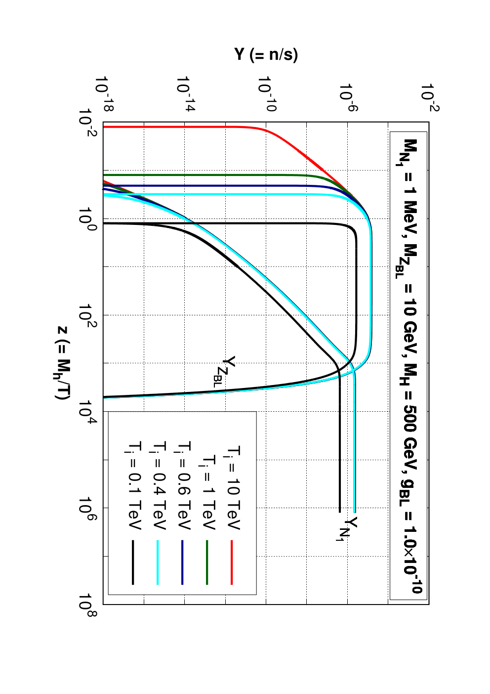
We now show the variation of Fig. 2 with different sets of chosen model parameters.

In Fig. 4(a) we show the variation of $Y_{Z_{\rm BL}}$ and $Y_{N_{1}}$ with $z$ for two different values of U(1)_B-L gauge coupling $g_{\rm BL}$. In this plot, we find that with increase in the value of $g_{\rm BL}$ the number density of $Z_{\rm BL}$ also increases initially. This is understandable, because the decay width $\Gamma_{H\rightarrow Z_{\rm BL}Z_{\rm BL}}$ increases with $g_{\rm BL}$, and hence resulting in an increased number density of the extra gauge boson. But the depletion rate of $Z_{\rm BL}$ (proportional to its total decay width) also increases with $g_{\rm BL}$, and hence will result in a faster fall of its comoving number density. This is also evident from the figure where the green line starts to fall earlier than the red one. On the other hand, the production rate of sterile neutrino dark matter ($N_{1}$) is proportional to $\Gamma_{Z_{\rm BL}\rightarrow N_{1}N_{1}}$ and $Y_{Z_{\rm BL}}$ (see Eq. ()) and both of these quantities increase with $g_{\rm BL}$. Therefore, the comoving number density of $N_{1}$ increases as the value of $g_{\rm BL}$ changes from $1\times 10^{-10}$ to $5\times 10^{-10}$.
In Fig. 4(b), we show the variation of $Y_{Z_{\rm BL}}$ and $Y_{N_{1}}$ with $z$ for two different values of $M_{H}$. Now, with a decrease in $M_{H}$, we expect a corresponding decrease in decay width $\Gamma_{H\rightarrow Z_{\rm BL}Z_{\rm BL}}$ ($Z_{\rm BL}$ production rate), and hence the initial number density of $Z_{\rm BL}$ will be smaller. This feature is seen in plot (b) where initially ($z\mathrel{\mathchoice{\vbox{\halign{\hfil$\displaystyle#$\hfil\cr<\cr\sim\cr}}}{\vbox{\halign{\hfil$\textstyle#$\hfil\cr<\cr\sim\cr}}}{\vbox{\halign{\hfil$\scriptstyle#$\hfil\cr<\cr\sim\cr}}}{\vbox{\halign{\hfil$\scriptscriptstyle#$\hfil\cr<\cr\sim\cr}}}}10^{3}$) $Y_{Z_{\rm BL}}$ for $M_{H}=500$ GeV (green line) is larger than that for $M_{H}=50$ GeV (red line). However, the total decay width of $Z_{\rm BL}$ (and consequently its depletion rate) does not depend on the mass of $H$. Hence both the red and green lines will start to fall off around the same time. Another noticeable change due to the variation of $M_{H}$ is that the width of the “plateau” becomes narrower with the decrease in mass difference between $M_{H}$ and $M_{Z_{\rm BL}}$. Further, as the $Y_{Z_{\rm BL}}$ increases with an increase in $M_{H}$, which in turn produces more $N_{1}$ (from the decay of $Z_{\rm BL}$) in the final state and hence the comoving number density $Y_{N_{1}}$ also increases with $M_{H}$.
In Fig. 4(c) we have shown the variation of $Y_{Z_{\rm BL}}$ and $Y_{N_{1}}$ for three different values of sterile neutrino dark matter mass. From this plot we find that there is not much variation in $Y_{Z_{\rm BL}}$ with changing $M_{N_{1}}$. This is because the decay width $\Gamma_{Z_{\rm BL}\rightarrow N_{1}N_{1}}$ is subdominant with respect to the other decays modes of $Z_{\rm BL}$. Increasing the mass of $N_{1}$ will lead to a further decrease of $\Gamma_{Z_{\rm BL}\rightarrow N_{1}N_{1}}$ and hence will not affect the depletion rate which is dominantly controlled by the other decay channels of $Z_{\rm BL}$. But since in this case (when other production channels of $N_{1}$ are switched off) $\Gamma_{Z_{\rm BL}\rightarrow N_{1}N_{1}}$ solely controls the production rate of $N_{1}$, $Y_{N_{1}}$ changes with $M_{N_{1}}$. It is seen from Fig. 4(c) that if we increase the sterile neutrino mass from 1 MeV to 4 GeV ($M_{N_{1}}$ tends to $M_{Z_{\rm BL}}/2$), then $Y_{N_{1}}$ decreases. The decrease in the decay width results in a corresponding decrease of $Y_{N_{1}}$ as expected. However we find no visible change in $Y_{N_{1}}$ when $M_{N_{1}}$ goes from 1 MeV to 100 MeV. This is because in both of these cases $M_{Z_{\rm BL}}\gg 2M_{N_{1}}$, therefore the decay width $\Gamma_{Z_{\rm BL}\rightarrow N_{1}N_{1}}$ and hence $Y_{N_{1}}$ is practically insensitive to $M_{N_{1}}$ ($M_{N_{1}}=$ 1 MeV to 100 MeV).
Finally, the effect of the variation of gauge boson mass $M_{Z_{\rm BL}}$ on $Y_{Z_{\rm BL}}$ and $Y_{N_{1}}$ is shown in Fig. 4(d). The increase in $M_{Z_{\rm BL}}$ results in the decrease of $\Gamma_{H\rightarrow Z_{\rm BL}Z_{\rm BL}}$ and an increase of $\Gamma_{Z_{\rm BL}\rightarrow all}$, which is manifested through a smaller rise and a faster fall of $Y_{Z_{\rm BL}}$. This nature of $Y_{Z_{\rm BL}}$ is corroborated in the plot as well, where $M_{Z_{\rm BL}}$ varies from 10 GeV (red line) to 100 GeV (green line). On the other hand the quantity $Y_{N_{1}}$ follows the evolution of $Y_{Z_{\rm BL}}$ in the usual way as discussed earlier. Since all these cases were shown to demonstrate the validity of the coupled Boltzmann equations, for simplicity the active sterile mixing angle ($\alpha$) is set to zero.

In order to compute the relic abundance ($\Omega_{N_{1}}h^{2}$) of the lightest sterile neutrino ($N_{1}$) we need to find the value of its comoving number density ($Y_{N_{1}}$) at the present epoch ($T=T_{0}$, $T_{0}\sim 2.73$ K). The value of $Y_{N_{1}}(T_{0})$ can be obtained by solving the two coupled Boltzmann equations (Eqs. (, ), which we have discussed elaborately in Section 4. The expression of $\Omega_{N_{1}}h^{2}$ in terms of $Y_{N_{1}}(T_{0})$ is given by [68],

$\displaystyle\Omega_{N_{1}}h^{2}=2.755\times 10^{8}\left(\frac{M_{N_{1}}}{\rm GeV}\right)Y_{N_{1}}(T_{0})\,\,.$

(38)

In this work, we take all decay and annihilation channels of both SM as well as BSM particles for the production of $N_{1}$. In Fig. 6 we show the relative contributions to $\Omega_{N_{1}}h^{2}$ from $W^{\pm}$ (red solid line) and $Z_{\rm BL}$ decay (green solid line) for some chosen sets of model parameters. The total relic abundance of $N_{1}$ is also shown by the blue solid line. For some combinations of model parameters we find $W^{\pm}$ decay can be the leading production channel of $N_{1}$ (plot (a)) while for some others it can be the subleading one (plot (c)). However in all three plots (a-c) of Fig. 6, the total relic density of $N_{1}$ has the saturation value $\sim 0.12$ which is in conformity with the value of dark matter relic density measured by the satellite borne experiment Planck.

In plot (b) of Fig. 6 we show a situation when the relative contributions to $\Omega_{N_{1}}h^{2}$ from both $W^{\pm}$ and $Z_{\rm BL}$ decays are equal. In this case we have adopted the following values of relevant model parameters: $g_{\rm BL}=3.07\times 10^{-11}$, $\alpha=4.74\times 10^{-10}$ rad, $M_{Z_{\rm BL}}=10$ GeV and $M_{H}=500$ GeV. For this set of model parameters we have also listed the fractional contributions to $\Omega_{N_{1}}h^{2}$ arising from all the possible decay and annihilation channels in Table 1, 2.

From Table 1 it is seen that for the small values of $g_{\rm BL}\sim 10^{-11}$ and $\alpha\sim 10^{-10}$ (which are required for the non-thermality of $N_{1}$) the contributions of other production channels of $N_{1}$ through the decays of $Z$, $H$ and $h$ are negligible. Similarly, Table 2 shows that within this adopted ranges of model parameters the annihilation processes of SM as well as BSM particles do not contribute significantly to the production of sterile neutrino dark matter $N_{1}$ and hence we can safely consider the decays of $W^{\pm}$ and $Z_{\rm BL}$ as the two most efficient production mechanisms of $N_{1}$.

In Fig. 7, we plot the allowed values of $\rm B-L$ gauge coupling $g_{\rm BL}$ and active sterile mixing angle $\alpha$ which satisfy the relic density criteria ($0.1172\leq\Omega_{N_{1}}h^{2}\leq 0.1226$) [2]. During the computation of Fig. 7 we have varied the relevant parameters in the following range.

$\displaystyle\begin{array}[]{cccccc}0.1\text{ GeV}&\leq&M_{Z_{\rm BL}}&\leq&250\text{ GeV}\,\,,\\ 1.2\text{ MeV}&\leq&M_{N_{1}}&\leq&10\text{ MeV}\,\,,\\ 10^{-8}&\leq&g_{\rm BL}&\leq&10^{-15}\,\,,\\ 10^{-7}\text{ rad}&\leq&\alpha&\leq&10^{-17}\text{ rad}\,\,,\end{array}$

and we have kept the mass of the extra Higgs boson $H$ fixed at 500 GeV. From Fig. 7, we see that for very small values of the extra gauge coupling $g_{\rm BL}$ ($\sim 10^{-12}\,\,{\rm to}\,\,10^{-15}$) the relic density condition of $N_{1}$ is always satisfied for a active-sterile mixing angle $\alpha\sim 10^{-10}$ rad. This is expected since for very small values of $g_{\rm BL}$ the production of $N_{1}$ from the decay of $Z_{\rm BL}$ is highly suppressed and in this situation decay of $W^{\pm}$ becomes the principle production channel, since the latter is not suppressed by the extra gauge coupling (see Eqs. (45), (47)). Earlier works about the non-thermal production of sterile neutrino have not touched upon this point in detail (production of $N_{1}$ from $W^{\pm}$ decay), since most of the previous authors have ignored the $N_{1}$ production mode from $W^{\pm}$ decay in their works by assuming extremely small values of active-sterile mixing angle $\alpha$. However, such an assumption needs careful attention when other couplings in the theory can also be very small. On the other hand for the higher values of $g_{\rm BL}$ ($\sim 10^{-9}\,\,{\rm to}\,\,10^{-11}$) the decay of $Z_{\rm BL}$ becomes the dominant contributor and hence in this case small values of $\alpha$ are required to suppress the contribution of $W^{\pm}$ decay to $\Omega_{N_{1}}h^{2}$ such that the total relic density of $N_{1}$ lies within the range prescribed by the Planck experiment. Since the production of sterile neutrino from $W^{\pm}$ decay depends only on the mixing angle $\alpha$, in Fig. 7 we get only a narrow band of $\alpha$ which satisfies the relic density of $N_{1}$ (for small values of $g_{\rm BL}$). But when $Z_{\rm BL}$ is the main production channel of $N_{1}$ then for a given $g_{\rm BL}$ and $\alpha$ we can make $N_{1}$ to satisfy the relic density by adjusting the $Z_{\rm BL}$ mass. Hence we get a relatively wider band of allowed values of $g_{\rm BL}$ for a fixed $\alpha$. For the chosen mass range of sterile neutrino (i.e. $\mathcal{O}$(MeV)), from Fig. 7 we find that the maximum allowed value of $\alpha$ is $\sim 10^{-10}$ rad. Such a sterile neutrino is free from all the constraints arising from X-ray and BBN as seen from Fig. 1 of Ref. [24].

The allowed region in $M_{Z_{\rm BL}}-g_{\rm BL}$ plane is shown in Fig.  8. Like the previous plot in Fig. 7, here also all the points in $M_{Z_{\rm BL}}-g_{\rm BL}$ plane produce the correct relic density of $N_{1}$ ($0.1172\leq\Omega_{N_{1}}h^{2}\leq 0.1226$). In this case we have also varied the other relevant parameters ($M_{N_{1}}$, $\alpha$) in the range given in Eq. (5). From this figure it is seen that the allowed values of $g_{\rm BL}$ increases with $M_{Z_{\rm BL}}$. This nature of $M_{Z_{\rm BL}}-g_{\rm BL}$ plane can be explained in the following way. We know that the contribution of $Z_{\rm BL}$ to $Y_{N_{1}}$ depends on both $\Gamma_{Z_{\rm BL}\rightarrow N_{1}N_{1}}$ and $Y_{Z_{\rm BL}}$ (see Eq. ()) where the latter quantity increases with $\Gamma_{H\rightarrow Z_{\rm BL}Z_{\rm BL}}$ (Eq. ()) as the extra gauge bosons $Z_{\rm BL}$ are produced mainly from the decay of $H$. However the decay width $\Gamma_{H\rightarrow Z_{\rm BL}Z_{\rm BL}}$ is suppressed by $M_{Z_{\rm BL}}^{-2}$ and thereby reducing the comoving number density of $Z_{\rm BL}$ with its mass (see Eq. (67) and Fig. 5(d)). In order to keep the contribution to $\Omega_{N_{1}}h^{2}$ arising from $Z_{\rm BL}$ decay unaltered, this decrement in $Y_{Z_{\rm BL}}$ must be compensated by a corresponding increment in $\Gamma_{Z_{\rm BL}\rightarrow N_{1}N_{1}}$ which is proportional to $g_{\rm BL}^{2}$ (Eq. (47)). Hence with an increase in $M_{Z_{\rm BL}}$, $g_{\rm BL}$ should also increase to satisfy the relic density constraint.

Simulations using the standard $\Lambda\rm CDM$ cosmology requires that most of the dark matter candidates should be cold to satisfy constraints from the structure formation [69, 70]. In our case, to get an idea about the coldness of the sterile neutrino dark matter we try to compute its free-steaming length defined by [63]:

$\displaystyle\lambda_{\rm fs}=\int_{t_{in}}^{t_{0}}\dfrac{\langle v(t)\rangle}{a(t)}\,dt\,,$

where $t_{in}$ is the initial time, $t_{0}$ is the present time, $v(t)$ is the mean velocity of the dark matter, and $a(t)$ is the scale factor of the Universe. Following Ref. [43], the hot, cold and warm dark matters are classified as:

	$\displaystyle\rm Cold\,\,Dark\,\,Matter\,\,(CDM)$	$\displaystyle:$	$\displaystyle\lambda_{\rm fs}<0.01\,\rm Mpc$
	$\displaystyle\rm Warm\,\,Dark\,\,Matter\,\,(WDM)$	$\displaystyle:$	$\displaystyle 0.01\,\rm Mpc<\lambda_{\rm fs}<0.1\,\rm Mpc$
	$\displaystyle\rm Hot\,\,Dark\,\,Matter\,\,(HDM)$	$\displaystyle:$	$\displaystyle\lambda_{\rm fs}>0.1\rm\,Mpc$

For the case where both $W^{\pm}$ and $Z_{\rm BL}$ contribute equally to the final dark matter relic density (Fig. 6b), we have calculated the free-streaming length for dark matter produced from $W^{\pm}$ as well as $Z_{\rm BL}$ decay separately. In both the cases we find that $\lambda_{\rm fs}^{W^{\pm}}\sim 0.003$ Mpc and $\lambda_{\rm fs}^{Z_{\rm BL}}\sim 0.007\,\,{\rm Mpc}$. Hence following the above classification of hot, cold and warm dark matter, we find that all of our sterile neutrino is cold and thus satisfying the structure formation constraints.

References

- [1] G. Hinshaw et al. [WMAP Collaboration], “Nine-Year Wilkinson Microwave Anisotropy Probe (WMAP) Observations: Cosmological Parameter Results”, Astrophys. J. Suppl. 208, 19 (2013) [arXiv:1212.5226 [astro-ph.CO]].
- [2] P. A. R. Ade et al. [Planck Collaboration], “Planck 2015 results. XIII. Cosmological parameters”, arXiv:1502.01589 [astro-ph.CO].
- [3] Y. Sofue and V. Rubin, “Rotation curves of spiral galaxies”, Ann. Rev. Astron. Astrophys. 39, 137 (2001) [astro-ph/0010594].
- [4] M. Bartelmann and P. Schneider, “Weak gravitational lensing”, Phys. Rept. 340, 291 (2001) [astro-ph/9912508].
- [5] D. Clowe, A. Gonzalez and M. Markevitch, “Weak lensing mass reconstruction of the interacting cluster 1E0657-558: Direct evidence for the existence of dark matter”, Astrophys. J. 604, 596 (2004) [astro-ph/0312273].
- [6] G. Jungman, M. Kamionkowski and K. Griest, “Supersymmetric dark matter”, Phys. Rept. 267, 195 (1996) [hep-ph/9506380].
- [7] D. S. Akerib et al. [LUX Collaboration], “Improved Limits on Scattering of Weakly Interacting Massive Particles from Reanalysis of 2013 LUX Data”, Phys. Rev. Lett. 116, no. 16, 161301 (2016) [arXiv:1512.03506 [astro-ph.CO]].
- [8] E. Aprile et al. [XENON100 Collaboration], “Dark Matter Results from 225 Live Days of XENON100 Data”, Phys. Rev. Lett. 109, 181301 (2012) [arXiv:1207.5988 [astro-ph.CO]].
- [9] E. Aprile et al. [XENON Collaboration], “Physics reach of the XENON1T dark matter experiment”, JCAP 1604, no. 04, 027 (2016) [arXiv:1512.07501 [physics.ins-det]].
- [10] D. S. Akerib et al. [LZ Collaboration], “LUX-ZEPLIN (LZ) Conceptual Design Report”, arXiv:1509.02910 [physics.ins-det].
- [11] C. E. Aalseth et al., “The DarkSide Multiton Detector for the Direct Dark Matter Search”, Adv. High Energy Phys. 2015, 541362 (2015).
- [12] A. Drukier and L. Stodolsky, “Principles and Applications of a Neutral Current Detector for Neutrino Physics and Astronomy”, Phys. Rev. D 30, 2295 (1984).
- [13] P. Cushman et al., “Working Group Report: WIMP Dark Matter Direct Detection”, arXiv:1310.8327 [hep-ex].
- [14] W. C. Haxton, R. G. Hamish Robertson and A. M. Serenelli, “Solar Neutrinos: Status and Prospects”, Ann. Rev. Astron. Astrophys. 51, 21 (2013) [arXiv:1208.5723 [astro-ph.SR]].
- [15] F. Mayet et al., “A review of the discovery reach of directional Dark Matter detection”, Phys. Rept. 627, 1 (2016) [arXiv:1602.03781 [astro-ph.CO]].
- [16] L. Covi, J. E. Kim and L. Roszkowski, “Axinos as cold dark matter”, Phys. Rev. Lett. 82, 4180 (1999) [hep-ph/9905212].
- [17] L. Covi, H. B. Kim, J. E. Kim and L. Roszkowski, “Axinos as dark matter”, JHEP 0105, 033 (2001) [hep-ph/0101009].
- [18] K. Y. Choi, J. E. Kim and L. Roszkowski, “Review of axino dark matter”, J. Korean Phys. Soc. 63, 1685 (2013) [arXiv:1307.3330 [astro-ph.CO]].
- [19] R. Kallosh, L. Kofman, A. D. Linde and A. Van Proeyen, “Gravitino production after inflation”, Phys. Rev. D 61, 103503 (2000) [hep-th/9907124].
- [20] G. F. Giudice, A. Riotto and I. Tkachev, “Thermal and nonthermal production of gravitinos in the early universe”, JHEP 9911, 036 (1999) [hep-ph/9911302].
- [21] E. W. Kolb, D. J. H. Chung and A. Riotto, “WIMPzillas! ”, In *Heidelberg 1998, Dark matter in astrophysics and particle physics 1998* 592-614 [hep-ph/9810361].
- [22] H. Baer, K. Y. Choi, J. E. Kim and L. Roszkowski, “Dark matter production in the early Universe: beyond the thermal WIMP paradigm”, Phys. Rept. 555, 1 (2015) [arXiv:1407.0017 [hep-ph]].
- [23] L. J. Hall, K. Jedamzik, J. March-Russell and S. M. West, “Freeze-In Production of FIMP Dark Matter”, JHEP 1003, 080 (2010) [arXiv:0911.1120 [hep-ph]].
- [24] B. Shakya, “Sterile Neutrino Dark Matter from Freeze-In”, Mod. Phys. Lett. A 31, no. 06, 1630005 (2016) [arXiv:1512.02751 [hep-ph]].
- [25] J. McDonald, “Thermally generated gauge singlet scalars as selfinteracting dark matter”, Phys. Rev. Lett. 88, 091304 (2002) [hep-ph/0106249].
- [26] C. E. Yaguna, “The Singlet Scalar as FIMP Dark Matter”, JHEP 1108, 060 (2011) [arXiv:1105.1654 [hep-ph]].
- [27] A. Biswas, D. Majumdar and P. Roy, “Nonthermal two component dark matter model for Fermi-LAT -ray excess and 3.55 keV X-ray line”, JHEP 1504, 065 (2015) [arXiv:1501.02666 [hep-ph]].
- [28] F. Elahi, C. Kolda and J. Unwin, “UltraViolet Freeze-in”, JHEP 1503, 048 (2015) [arXiv:1410.6157 [hep-ph]].
- [29] S. B. Roland, B. Shakya and J. D. Wells, “Neutrino Masses and Sterile Neutrino Dark Matter from the PeV Scale”, Phys. Rev. D 92, no. 11, 113009 (2015) [arXiv:1412.4791 [hep-ph]].
- [30] P. S. Bhupal Dev, A. Mazumdar and S. Qutub, “Constraining Non-thermal and Thermal properties of Dark Matter”, Front. in Phys. 2, 26 (2014) [arXiv:1311.5297 [hep-ph]].
- [31] M. Endo and F. Takahashi, “Non-thermal Production of Dark Matter from Late-Decaying Scalar Field at Intermediate Scale”, Phys. Rev. D 74, 063502 (2006) [hep-ph/0606075].
- [32] M. Shaposhnikov and I. Tkachev, “The nuMSM, inflation, and dark matter”, Phys. Lett. B 639, 414 (2006) [hep-ph/0604236].
- [33] N. Okada and O. Seto, “Higgs portal dark matter in the minimal gauged model”, Phys. Rev. D 82, 023507 (2010) [arXiv:1002.2525 [hep-ph]].
- [34] T. Basak and T. Mondal, “Constraining Minimal model from Dark Matter Observations”, Phys. Rev. D 89, 063527 (2014) [arXiv:1308.0023 [hep-ph]].
- [35] W. Rodejohann and C. E. Yaguna, “Scalar dark matter in the B-L model”, JCAP 1512, no. 12, 032 (2015) [arXiv:1509.04036 [hep-ph]].
- [36] A. Biswas, S. Choubey and S. Khan, “Galactic Gamma Ray Excess and Dark Matter Phenomenology in a Model”, arXiv:1604.06566 [hep-ph].
- [37] S. Dodelson and L. M. Widrow, “Sterile-neutrinos as dark matter”, Phys. Rev. Lett. 72, 17 (1994) [hep-ph/9303287].
- [38] R. Essig et al., “Constraining Light Dark Matter with Diffuse X-Ray and Gamma-Ray Observations”, JHEP 1311, 193 (2013) [arXiv:1309.4091 [hep-ph]].
- [39] X. D. Shi and G. M. Fuller, “A New dark matter candidate: Nonthermal sterile neutrinos”, Phys. Rev. Lett. 82, 2832 (1999) [astro-ph/9810076].
- [40] S. B. Roland, B. Shakya and J. D. Wells, “PeV neutrinos and a 3.5 keV x-ray line from a PeV-scale supersymmetric neutrino sector”, Phys. Rev. D 92, no. 9, 095018 (2015) [arXiv:1506.08195 [hep-ph]].
- [41] K. Kadota, “Sterile neutrino dark matter in warped extra dimensions”, Phys. Rev. D 77, 063509 (2008) [arXiv:0711.1570 [hep-ph]].
- [42] M. Frigerio and C. E. Yaguna, “Sterile Neutrino Dark Matter and Low Scale Leptogenesis from a Charged Scalar”, Eur. Phys. J. C 75, no. 1, 31 (2015) [arXiv:1409.0659 [hep-ph]].
- [43] A. Merle, V. Niro and D. Schmidt, “New Production Mechanism for keV Sterile Neutrino Dark Matter by Decays of Frozen-In Scalars”, JCAP 1403, 028 (2014) [arXiv:1306.3996 [hep-ph]].
- [44] A. Merle and M. Totzauer, “keV Sterile Neutrino Dark Matter from Singlet Scalar Decays: Basic Concepts and Subtle Features”, JCAP 1506, 011 (2015) [arXiv:1502.01011 [hep-ph]].
- [45] B. Shuve and I. Yavin, “Dark matter progenitor: Light vector boson decay into sterile neutrinos”, Phys. Rev. D 89, no. 11, 113004 (2014) [arXiv:1403.2727 [hep-ph]].
- [46] K. Kaneta, Z. Kang and H. S. Lee, “Right-handed neutrino dark matter under the B-L gauge interaction”, arXiv:1606.09317 [hep-ph].
- [47] G. Gelmini, S. Palomares-Ruiz and S. Pascoli, “Low reheating temperature and the visible sterile neutrino”, Phys. Rev. Lett. 93, 081302 (2004) [astro-ph/0403323].
- [48] G. Gelmini, E. Osoba, S. Palomares-Ruiz and S. Pascoli, “MeV sterile neutrinos in low reheating temperature cosmological scenarios”, JCAP 0810, 029 (2008) [arXiv:0803.2735 [astro-ph]].
- [49] S. Khalil and O. Seto, “Sterile neutrino dark matter in B-L extension of the standard model and galactic 511-keV line”, JCAP 0810, 024 (2008) [arXiv:0804.0336 [hep-ph]].
- [50] J. Knodlseder et al., “Early SPI / INTEGRAL contraints on the morphology of the 511 keV line emission in the 4th galactic quadrant”, Astron. Astrophys. 411, L457 (2003) [astro-ph/0309442].
- [51] G. Aad et al. [ATLAS Collaboration], “Observation of a new particle in the search for the Standard Model Higgs boson with the ATLAS detector at the LHC”, Phys. Lett. B 716, 1 (2012) [arXiv:1207.7214 [hep-ex]].
- [52] S. Chatrchyan et al. [CMS Collaboration], “Observation of a new boson at a mass of 125 GeV with the CMS experiment at the LHC”, Phys. Lett. B 716, 30 (2012) [arXiv:1207.7235 [hep-ex]].
- [53] T. Mondal and T. Basak, “Class of Higgs-portal Dark Matter models in the light of gamma-ray excess from Galactic center”, Phys. Lett. B 744, 208 (2015) [arXiv:1405.4877 [hep-ph]].
- [54] A. Hook, E. Izaguirre and J. G. Wacker, “Model Independent Bounds on Kinetic Mixing”, Adv. High Energy Phys. 2011, 859762 (2011) [arXiv:1006.0973 [hep-ph]].
- [55] L. Basso, A. Belyaev, S. Moretti and C. H. Shepherd-Themistocleous, “Phenomenology of the minimal B-L extension of the Standard model: Z’ and neutrinos”, Phys. Rev. D 80, 055030 (2009) [arXiv:0812.4313 [hep-ph]].
- [56] M. Carena, A. Daleo, B. A. Dobrescu and T. M. P. Tait, “ gauge bosons at the Tevatron”, Phys. Rev. D 70, 093009 (2004) [hep-ph/0408098].
- [57] G. Cacciapaglia, C. Csaki, G. Marandella and A. Strumia, “The Minimal Set of Electroweak Precision Parameters”, Phys. Rev. D 74, 033011 (2006) [hep-ph/0604111].
- [58] G. Aad et al. [ATLAS Collaboration], “Search for high-mass dilepton resonances in pp collisions at TeV with the ATLAS detector”, Phys. Rev. D 90, no. 5, 052005 (2014) [arXiv:1405.4123 [hep-ex]].
- [59] P. Gondolo and G. Gelmini, “Cosmic abundances of stable particles: Improved analysis”, Nucl. Phys. B 360, 145 (1991).
- [60] G. Arcadi and L. Covi, “Minimal Decaying Dark Matter and the LHC ”, JCAP 1308, 005 (2013) [arXiv:1305.6587 [hep-ph]].
- [61] K. A. Olive et al. [Particle Data Group Collaboration], “Review of Particle Physics”, Chin. Phys. C 38, 090001 (2014).
- [62] P. Bechtle, S. Heinemeyer, O. Stål, T. Stefaniak and G. Weiglein, “Probing the Standard Model with Higgs signal rates from the Tevatron, the LHC and a future ILC”, JHEP 1411, 039 (2014) [arXiv:1403.1582 [hep-ph]].
- [63] A. Boyarsky, J. Lesgourgues, O. Ruchayskiy and M. Viel, “Lyman-alpha constraints on warm and on warm-plus-cold dark matter models”, JCAP 0905, 012 (2009) [arXiv:0812.0010 [astro-ph]].
- [64] U. Seljak, A. Makarov, P. McDonald and H. Trac, “Can sterile neutrinos be the dark matter? ”, Phys. Rev. Lett. 97, 191303 (2006) [astro-ph/0602430].
- [65] A. Boyarsky, J. Lesgourgues, O. Ruchayskiy and M. Viel, “Realistic sterile neutrino dark matter with keV mass does not contradict cosmological bounds”, Phys. Rev. Lett. 102, 201304 (2009) [arXiv:0812.3256 [hep-ph]].
- [66] K. Abazajian, G. M. Fuller and M. Patel, “Sterile neutrino hot, warm, and cold dark matter”, Phys. Rev. D 64, 023501 (2001) [astro-ph/0101524].
- [67] K. S. Babu and R. N. Mohapatra, “7 keV Scalar Dark Matter and the Anomalous Galactic X-ray Spectrum”, Phys. Rev. D 89, 115011 (2014) [arXiv:1404.2220 [hep-ph]].
- [68] J. Edsjo and P. Gondolo, “Neutralino relic density including coannihilations”, Phys. Rev. D 56, 1879 (1997) [hep-ph/9704361].
- [69] J. R. Primack, “Dark matter and structure formation”, astro-ph/9707285.
- [70] J. Diemand and B. Moore, “The structure and evolution of cold dark matter halos”, Adv. Sci. Lett. 4, 297 (2011) [arXiv:0906.4340 [astro-ph.CO]].
- [71] T. Siegert et al., “Gamma-ray spectroscopy of Positron Annihilation in the Milky Way”, Astron. Astrophys. 586, A84 (2016) [arXiv:1512.00325 [astro-ph.HE]].
- [72] J. Knodlseder et al., “The All-sky distribution of 511 keV electron-positron annihilation emission”, Astron. Astrophys. 441, 513 (2005) [astro-ph/0506026].
- [73] L. Boubekeur, S. Dodelson and O. Vives, “Cold Positrons from Decaying Dark Matter”, Phys. Rev. D 86, 103520 (2012) [arXiv:1206.3076 [astro-ph.CO]].
- [74] E. J. Chun and H. B. Kim, “Axino Light Dark Matter and Neutrino Masses with R-parity Violation”, JHEP 0610, 082 (2006) [hep-ph/0607076].
- [75] D. P. Finkbeiner and N. Weiner, “Exciting Dark Matter and the INTEGRAL/SPI 511 keV signal”, Phys. Rev. D 76, 083519 (2007) [astro-ph/0702587].
- [76] D. Hooper et al., “Possible evidence for MeV dark matter in dwarf spheroidals”, Phys. Rev. Lett. 93, 161302 (2004) [astro-ph/0311150].
- [77] N. Prantzos et al., “The 511 keV emission from positron annihilation in the Galaxy”, Rev. Mod. Phys. 83, 1001 (2011) [arXiv:1009.4620 [astro-ph.HE]].
- [78] R. J. Wilkinson, A. C. Vincent, C. Boehm and C. McCabe, “Ruling out the light WIMP explanation of the galactic 511 keV line”, arXiv:1602.01114 [astro-ph.CO].
- [79] C. Picciotto and M. Pospelov, “Unstable relics as a source of galactic positrons”, Phys. Lett. B 605, 15 (2005) [hep-ph/0402178].
- [80] Y. Ascasibar, P. Jean, C. Boehm and J. Knoedlseder, “Constraints on dark matter and the shape of the Milky Way dark halo from the 511-keV line”, Mon. Not. Roy. Astron. Soc. 368, 1695 (2006) [astro-ph/0507142].
- [81] C. Boehm, D. Hooper, J. Silk, M. Casse and J. Paul, “MeV dark matter: Has it been detected? ”, Phys. Rev. Lett. 92, 101301 (2004) [astro-ph/0309686].
- [82] M. Cirelli et al., “PPPC 4 DM ID: A Poor Particle Physicist Cookbook for Dark Matter Indirect Detection”, JCAP 1103, 051 (2011) Erratum: [JCAP 1210, E01 (2012)] [arXiv:1012.4515 [hep-ph]].
- [83] A. Denner et al., “Standard Model Higgs-Boson Branching Ratios with Uncertainties”, Eur. Phys. J. C 71, 1753 (2011) [arXiv:1107.5909 [hep-ph]].