∎

Mixtures of Bivariate von Mises Distributions with Applications to Modelling of Protein Dihedral Angles

Journal: Machine Learning

Parthan Kasarapu Affiliation: Faculty of Information Technology, Monash University, VIC 3800, Australia E-mail: parthan.kasarapu@monash.edu

Abstract

The modelling of empirically observed data is commonly done using mixtures of probability distributions. In order to model angular data, directional probability distributions such as the bivariate von Mises (BVM) is typically used. The critical task involved in mixture modelling is to determine the optimal number of component probability distributions. We employ the Bayesian information-theoretic principle of minimum message length (MML) to distingush mixture models by balancing the trade-off between the model’s complexity and its goodness-of-fit to the data. We consider the problem of modelling angular data resulting from the spatial arrangement of protein structures using BVM distributions. The main contributions of the paper include the development of the mixture modelling apparatus along with the MML estimation of the parameters of the BVM distribution. We demonstrate that statistical inference using the MML framework supersedes the traditional methods and offers a mechanism to objectively determine models that are of practical significance.

Keywords:

mixture modelling directional statistics von Mises minimum message length

1 Introduction

The efficient and accurate modelling of data is crucial to support reliable analyses and to improve the solution to related problems. Mixture probability distributions are commonly used in machine learning applications to model the underlying, often unknown, distribution of the data (Titterington et al, 1985; McLachlan and Basford, 1988; Jain et al, 2000). They are widely used to describe data arising in various domains such as astronomy, biology, ecology, engineering, and economics, amongst many others (McLachlan and Peel, 2000). In order to describe the given data, the problem of selecting a suitable statistical model has to be carefully addressed.

The problem of mixture modelling is associated with the difficult task of selecting the optimal number of mixture components and estimating the parameters of the constituent probability distributions. Mixtures with varying number of component distributions differ in their model complexities and their goodness-of-fit to the data. An increase in the complexity of the mixture model, corresponding to an increase in the model parameters, leads to better quality of fit to the data. Various criteria have been proposed to address the trade-off arising due to these two conflicting objectives (Akaike, 1974; Schwarz, 1978; Rissanen, 1978; Bozdogan, 1993; Oliver et al, 1996; Roberts et al, 1998; Biernacki et al, 2000; Figueiredo and Jain, 2002). As explained in Kasarapu and Allison (2015), these methods are not completely effective in addressing this trade-off as the model complexity is approximated as a function of the number of parameters and not the actual parameters themselves. While some of the methods aim to tune the criteria used to evaluate a mixture model (Akaike, 1974; Schwarz, 1978; Rissanen, 1978; Roberts et al, 1998; Biernacki et al, 2000), they do not provide an associated search strategy to infer the optimal number of mixture components. The methods that incorporate a rigorous search method for the mixture components are based on dynamic perturbations of the mixture model (Ueda et al, 2000; Figueiredo and Jain, 2002; Kasarapu and Allison, 2015). A thorough review of the various approaches to mixture modelling methods and their limitations is outlined in Kasarapu and Allison (2015).

The strategies based on Bayesian inference, and more specifically, using the minimum message length (MML) framework have increasingly found support in mixture modelling tasks (Wallace and Boulton, 1968; Wallace, 1986; Roberts et al, 1998; Figueiredo and Jain, 2002; Kasarapu and Allison, 2015). The MML-based inference framework decomposes a modelling problem into two parts: the first part determines the model complexity by encoding all the parameters of the model, and the second part corresponds to encoding of the observed data using the chosen parameters. Thus, a two-part message length is obtained for a model under consideration. A model that results in the least total message length is then determined to be the optimal model under this framework (Oliver and Baxter, 1994).

The MML-based search method developed by Kasarapu and Allison (2015) is demonstrated to outperform the traditionally used approaches and is the current state-of-the art. Kasarapu and Allison (2015) have designed the mixture modelling apparatus to include Gaussian distributions to model data in the Euclidean space and von Mises-Fisher (vMF) distributions to model directional data distributed on the surface of a sphere. While Gaussian mixtures are ubiquitously used because of their computational tractability (McLachlan and Peel, 2000), they are ineffective to model directional data. In this context, analogues of the Gaussian distribution defined on the surfaces of the appropriate Reimannian manifolds are typically considered. The vMF is the most fundamental directional probability distribution defined on the spherical surface. It is the spherical analogue of a symmetrical Gaussian wrapped around a unit hypersphere (Fisher, 1953; Watson and Williams, 1956) and is demonstrated to be useful in large-scale text clustering (Banerjee et al, 2003; Kasarapu and Allison, 2015) and gene expression analyses (Banerjee et al, 2005). A general form of the vMF distribution is the Fisher-Bingham ( $\text{FB}_{5}$ ) distribution which is used to model asymmetrically distributed data on the spherical surface (Kent, 1982). Mixtures of $\text{FB}_{5}$ distributions have been employed by Peel et al (2001) to identify joint sets in rock masses, and by Hamelryck et al (2006) to sample random protein conformations. The $\text{FB}_{5}$ distribution has increasingly found support in machine learning tasks for structural bioinformatics (Kent and Hamelryck, 2005; Boomsma et al, 2006; Hamelryck, 2009).

A two-dimensional version of the vMF distributions called the von Mises circular is used to model data distributed on the boundary of a circle. Each data point on the circle has a domain $[-\pi,\pi)$ . If such data occur as pairs, then the resulting manifold in three dimensions would be a torus. The bivariate von Mises (BVM) distributions are used to model such data distributed on the toroidal surface and serve as the Gaussian analogue. Motivated by its practical applications in bioinformatics, the BVM distributions are widely studied. The mixtures of BVM distributions have been previously used in modelling protein dihedral angles (Dowe et al, 1996; Mardia et al, 2007; Mardia et al, 2008). However, these approaches have some limitations. Dowe et al (1996) treat the pairs of angles to be independent of each other and do not account for their correlation. This is akin to conflating two von Mises circular distributions together. As explained in Section 4, such an approximation leads to inefficient mixtures. Although Mardia et al (2007) use BVM distributions that account for the correlation between the angular pairs, they do not have a rigorous search method to determine the optimal mixtures. This limits their ability to correctly distinguish among models that, while being of different type, have the same number of model parameters.

This paper develops the mixture modelling apparatus to address these limitations using the MML framework. Further, different variants of the BVM distribution obtained by constraining some of its characterizing parameters (see Section 2). Mardia et al (2007) have evaluated the utility of these variants in the context of modelling the protein dihedral angles. We adopt the MML principle in objectively assessing the mixture distributions of these variants (see Section 4). We have developed a search method to determine the optimal number of mixture components and their parameters that describe the given data in a completely unsupervised setting. The use of the MML modelling paradigm and our proposed search method is explored on real-world data corresponding to the dihedral, that is, torsion angles of protein structures. We demonstrate that mixtures of BVM distributions facilitate the design of reliable computational models for protein structural data.

In addition to determining the optimal number of mixture components, the parameters of the individual component distributions need to be estimated. Traditionally, the optimum parameters are obtained by maximum likelihood (ML) or Bayesian maximum a posteriori probability (MAP) estimation. For a mixture distribution, the parameters are estimated by maximizing the likelihood of the data by employing an expectation-maximization (EM) algorithm that iteratively updates the mixture parameters (Dempster et al, 1977). The key differences between ML, MAP and MML-based estimation is: (1) unlike ML, MML uses a prior over the parameters and considers their precision while encoding; (2) unlike MAP, MML estimators are invariant under non-linear transformations of the parameters (Oliver and Baxter, 1994). The estimation of parameters using ML ignores the cost of stating the parameters, and MAP based estimation uses the probability density of parameters instead of their probability measure. In contrast, the MML inference process takes into account the optimal precision to which parameters should be stated and uses it to determine a corresponding probability value. Parameter estimation using the MML framework has been carried out on various probability distributions (Wallace, 2005). Kasarapu and Allison (2015) have demonstrated that the MML estimators outperform the traditionally used estimators in the case of Gaussian and vMF distributions. Furthermore, for a $\text{FB}_{5}$ distribution, Kasarapu (2015) have shown that the MML estimators have lower bias and error as compared to the ML and MAP estimators.

Contributions: The main contributions of this paper are as follows:

•

We derive the MML-based estimates of the parameters of a BVM distribution. The MML estimators are demonstrated to have lower bias and mean squared error when compared to their traditional counterparts. We consider two variants of the BVM distribution, namely the Independent (Dowe et al, 1996) and the Sine variant (Singh et al, 2002).
•

We design a search method to infer the optimal number of BVM mixture components that best describe the angular data distributed on the toroidal surface.
•

We demonstrate the utility of the MML framework in determining the suitability of the two variants of the BVM distribution in modelling the protein dihedral angle data. We show that the Sine variant that includes the correlation term explains the data much more effectively than the Independent version.
•

We demonstrate the effectiveness of the mixture modelling method by applying it to cluster protein dihedral angles. We demonstrate that the resulting mixtures closely correspond to the commonly observed secondary structural regions in protein structures.

The rest of the chapter is organized as follows: Section 2 describes the BVM distribution, the Independent and the Sine variants, and their relevance in modelling data distributed on the toroidal surface. Section 3 describes the MML framework and outlines the differences between parameter estimation using ML, MAP and MML methods. It includes the derivation of the MML estimators of the parameters of the BVM distribution. We empirically demonstrate that the MML estimators outperform the traditionally used ML and MAP estimators by having lower bias and mean squared error. Section 4 discusses the search and inference of mixtures of bivariate von Mises (BVM) distributions using the MML framework. As a specific application, we employ the mixtures to model protein dihedral angles. We demonstrate that our search method is able to infer meaningful clusters that directly correspond to frequently occuring conformations in protein structures.

2 Bivariate von Mises probability distribution

The class of bivariate von Mises (BVM) distributions was introduced by Mardia (1975a); Mardia (1975b) to model data distributed on the surface of a 3D torus. The study of these distributions has been partly motivated by biological research, where it is required to model the protein dihedral angles (see Section 4.2). The probability density function of the BVM distribution has the general form

f(\mathbf{x};\bm{\Theta})\propto\exp\{\kappa_{1}\cos(\theta_{1}-\mu_{1})+\kappa_{2}\cos(\theta_{2}-\mu_{2})+(\cos\theta_{1},\,\sin\theta_{1})\mathbf{A}(\cos\theta_{2},\,\sin\theta_{2})^{T}\}

(1)

where $\mathbf{x}=(\theta_{1},\theta_{2})$ , such that $\theta_{1},\theta_{2}\in[-\pi,\pi)$ and the parameter vector $\bm{\Theta}=(\mu_{1},\mu_{2},\kappa_{1},\kappa_{2},\mathbf{A})$ , such that $\mu_{1},\mu_{2}\in[-\pi,\pi)$ are the mean angles, $\kappa_{1}\geq 0$ and $\kappa_{2}\geq 0$ are the concentration parameters, and $\mathbf{A}$ is a $2\times 2$ real-valued matrix. The term $\exp\{\kappa_{1}\cos(\theta_{1}-\mu_{1})\}$ corresponds to a von Mises distribution on a circle characterized by the parameters $\mu_{1}$ and $\kappa_{1}$ , Hence, the BVM distribution (Equation 1) can be explained as a product of two von Mises circular distributions, with an additional exponential term involving $\mathbf{A}$ , that accounts for the correlation.

The general form of the BVM distribution has 8 free parameters. In order to draw an analogy to the bivariate Gaussian distribution (with 5 free parameters), sub-models of the BVM distribution have been proposed by restricting the values that $\mathbf{A}$ can take (Jupp and Mardia, 1980). A 6-parameter version was explored by Rivest (1988) and has the form

	$\displaystyle f(\mathbf{x};\bm{\Theta})\propto\exp\{$	$\displaystyle\kappa_{1}\cos(\theta_{1}-\mu_{1})+\kappa_{2}\cos(\theta_{2}-\mu_{2})+\alpha\cos(\theta_{1}-\mu_{1})\cos(\theta_{2}-\mu_{2})$
		$\displaystyle+\beta\sin(\theta_{1}-\mu_{1})\sin(\theta_{2}-\mu_{2})\}$		(2)

In particular, when $\alpha=0$ and $\beta=\lambda$ , the above density reduces to the following 5-parameter version, which is called the BVM Sine model (Singh et al, 2002).

f(\mathbf{x};\bm{\Theta})=c(\kappa_{1},\kappa_{2},\lambda)^{-1}\exp\{\kappa_{1}\cos(\theta_{1}-\mu_{1})+\kappa_{2}\cos(\theta_{2}-\mu_{2})+\lambda\sin(\theta_{1}-\mu_{1})\sin(\theta_{2}-\mu_{2})\}

(3)

where $c(\kappa_{1},\kappa_{2},\lambda)$ is the normalization constant of the distribution defined as

\quad c(\kappa_{1},\kappa_{2},\lambda)=4\pi^{2}\sum_{j=0}^{\infty}\binom{2j}{j}\left(\frac{\lambda^{2}}{4\kappa_{1}\kappa_{2}}\right)^{j}I_{j}(\kappa_{1})I_{j}(\kappa_{2})

(4)

and $I_{v}$ is the modified Bessel function of first kind and order $v$ . The 5-parameter vector will be $\bm{\Theta}=(\mu_{1},\mu_{2},\kappa_{1},\kappa_{2},\lambda)$ where $\lambda$ is a real number. If $\lambda=0$ , the probability density function (Equation 3) will just be the product of two independent von Mises circular distributions, and corresponds to the case when there is no correlation between the two variables $\theta_{1}$ and $\theta_{2}$ . The probability density function in such a case is given as

f(\mathbf{x};\bm{\Theta})=c(\kappa_{1},\kappa_{2})^{-1}\exp\{\kappa_{1}\cos(\theta_{1}-\mu_{1})+\kappa_{2}\cos(\theta_{2}-\mu_{2})\}

(5)

where $c(\kappa_{1},\kappa_{2})$ is the normalization constant defined as $c(\kappa_{1},\kappa_{2})=\dfrac{1}{2\pi I_{0}(\kappa_{1})}\dfrac{1}{2\pi I_{0}(\kappa_{2})}$ . and corresponds to the product of the normalization constants for the respective von Mises circular distributions.

Alternatively, when $\alpha=-\beta$ , the form of Equation 2 results in a different reduced form called the BVM Cosine model (Mardia et al, 2007). The Sine and the Cosine models serve as natural analogues of the bivariate Gaussian distribution on the 3D torus. In fact, for huge concentrations, Singh et al (2002) approximate the Sine model to a bivariate Gaussian distribution with the $2\times 2$ covariance matrix $\mathbf{C}=[c_{ij}],i,j\in\{1,2\}$ , whose elements are given by

c_{11}=\frac{\kappa_{2}}{\kappa_{1}\kappa_{2}-\lambda^{2}},\quad c_{22}=\frac{\kappa_{1}}{\kappa_{1}\kappa_{2}-\lambda^{2}},\quad c_{12}=c_{21}=\frac{\lambda}{\kappa_{1}\kappa_{2}-\lambda^{2}}

The limiting case approximation is valid when $\kappa_{1}\kappa_{2}>\lambda^{2}$ . Also, from the covariance matrix, the correlation coefficient $\rho$ can be determined as (Pearson, 1895):

\rho=\frac{c_{12}}{\sqrt{c_{11}c_{22}}}=\frac{\lambda}{\sqrt{\kappa_{1}\kappa_{2}}}\quad\text{such that}\quad|\rho|<1

(6)

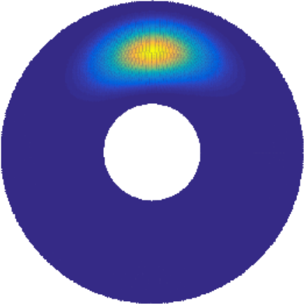
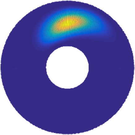
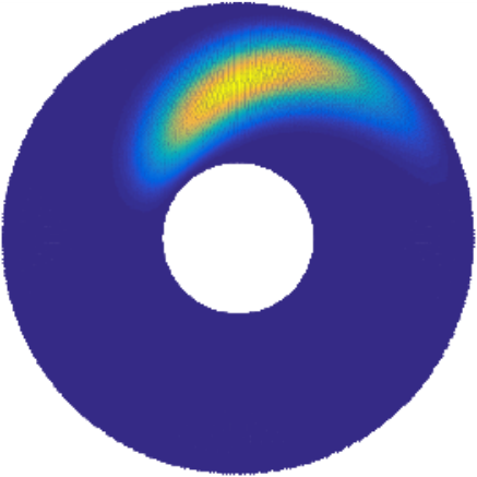
In order to better understand the interaction of $\kappa_{1},\kappa_{2},$ and the correlation coefficient $\rho$ , we provide an example in Figure 1, where the distribution is shown for values of $\rho=0.1$ (low correlation), $\rho=0.5$ (moderate correlation), and $\rho=0.9$ (high correlation). Note that $\rho$ can take negative values, in which case the resultant distribution will just be a reflection in some axis (Mardia et al, 2007).

(a)

\rho=0.1

(b)

\rho=0.5

(c)

\rho=0.9

Figure 1: BVM Sine model showing different correlations. The distribution has

\mu_{1}=\mu_{2}=\frac{\pi}{2}

and

\kappa_{1}=\kappa_{2}=10

. For each value of

\rho

, the corresponding value of

\lambda=\rho\sqrt{\kappa_{1}\kappa_{2}}

The modelling of directional data using the BVM Sine and Cosine models has been previously explored by Mardia et al (2007). For estimating the parameters of the distribution, maximum likelihood based optimization is used. We discuss ML and MAP based estimators, which are the traditionally used methods of parameter estimation.

2.1 Maximum likelihood parameter estimation

In applications involving modelling directional data using the BVM Sine distributions, the maximum likelihood (ML) estimates are typically used (Boomsma et al, 2006; Mardia et al, 2007; Mardia et al, 2008). For BVM Sine distributions, the moment and ML estimates are the same, as the BVM Sine distribution belongs to the exponential family of distributions (Mardia et al, 2008).

Given data $\mathcal{D}=\{\mathbf{x}_{1},\ldots,\mathbf{x}_{N}\}$ , where $\mathbf{x}_{i}=(\theta_{i1},\theta_{i2})$ , the ML estimates of the parameter vector $\bm{\Theta}=(\mu_{1},\mu_{2},\kappa_{1},\kappa_{2},\lambda)$ are obtained by minimizing the negative log-likelihood expression of the data given by

	$\displaystyle\mathcal{L}(\mathcal{D}\|\bm{\Theta})=$	$\displaystyle N\log c(\kappa_{1},\kappa_{2},\lambda)-\kappa_{1}\sum_{i=1}^{N}\cos(\theta_{i1}-\mu_{1})-\kappa_{2}\sum_{i=1}^{N}\cos(\theta_{i2}-\mu_{2})$
		$\displaystyle-\lambda\sum_{i=1}^{N}\sin(\theta_{i1}-\mu_{1})\sin(\theta_{i2}-\mu_{2})$		(7)

The ML estimates satisfy $\dfrac{\partial\mathcal{L}}{\partial\bm{\Theta}}=0$ . However, as no closed form soultions exist because of the complicated form of $c(\kappa_{1},\kappa_{2},\lambda)$ , an optimization library is used. We use NLopt¹¹ 1 http://ab-initio.mit.edu/nlopt, a non-linear optimization library, to compute the parameter estimates.

2.2 Maximum a posteriori probability (MAP) estimation

For an independent and identically distributed sample $\mathcal{D}$ , the MAP estimates are obtained by maximizing the posterior density $\Pr(\bm{\Theta}|\mathcal{D})$ . This requires the definition of a reasonable prior $\Pr(\bm{\Theta})$ on the parameter space. The MAP estimates are sensitive to the nature of parameterization of the probability distribution and this limitation is discussed here. We demonstrate that the MAP estimators are inconsistent and are subjective to the parameterization. We consider two alternative parameterizations in the case of the BVM Sine distribution.

Prior on the angular parameters $\mu_{1}$ and $\mu_{2}$ : Since $\mu_{1},\mu_{2}\in[-\pi,\pi)$ , a uniform prior can be assumed in this range for each of the means. Further, assuming $\mu_{1}$ and $\mu_{2}$ to be independent of each other, their joint prior will be $\Pr(\mu_{1},\mu_{2})=\dfrac{1}{4\pi^{2}}$ .

Prior on the scale parameters $\kappa_{1},\kappa_{2}$ , and $\lambda$ : As discussed for Equation 1, the BVM density function can be regarded as a product of two von Mises circular distributions with an additional term that captures the correlation. In the Bayesian analysis of the von Mises circular distribution, Wallace and Dowe (1994a) used the prior on the concentration parameter $\kappa$ as $\Pr(\kappa)=\dfrac{\kappa}{(1+\kappa^{2})^{3/2}}$ . In the current context of defining priors on $\kappa_{1}$ and $\kappa_{2}$ for a BVM distribution, we use the prior $\Pr(\kappa)$ . Assuming $\kappa_{1}$ and $\kappa_{2}$ to be independent of each other, the joint prior is given by

\Pr(\kappa_{1},\kappa_{2})=\frac{\kappa_{1}\kappa_{2}}{(1+\kappa_{1}^{2})^{3/2}(1+\kappa_{2}^{2})^{3/2}}

In order to define a reasonable prior on $\lambda$ , we use the fact that $\lambda^{2}<\kappa_{1}\kappa_{2}$ (see Equation 6). Hence, the conditional probability density of $\lambda$ is given as: $\Pr(\lambda|\kappa_{1},\kappa_{2})=\dfrac{1}{2\sqrt{\kappa_{1}\kappa_{2}}}$ . Therefore, the joint prior density of the scalar parameters $\kappa_{1},\kappa_{2}$ and $\lambda$ is

\Pr(\kappa_{1},\kappa_{2},\lambda)=\Pr(\kappa_{1},\kappa_{2})\Pr(\lambda|\kappa_{1},\kappa_{2})=\frac{\sqrt{\kappa_{1}\kappa_{2}}}{2(1+\kappa_{1}^{2})^{3/2}(1+\kappa_{2}^{2})^{3/2}}

Using the product of the priors for the angular and the scale parameters, that is, $\Pr(\mu_{1},\mu_{2})$ and $\Pr(\kappa_{1},\kappa_{2},\lambda)$ , the joint prior of the parameter vector $\bm{\Theta}$ , is given by

\Pr(\bm{\Theta})=\Pr(\mu_{1},\mu_{2},\kappa_{1},\kappa_{2},\lambda)=\frac{\sqrt{\kappa_{1}\kappa_{2}}}{8\pi^{2}(1+\kappa_{1}^{2})^{3/2}(1+\kappa_{2}^{2})^{3/2}}

(8)

The prior density $\Pr(\bm{\Theta})$ can be used along with the likelihood function to formulate the posterior density as the product of the prior and the likelihood function, that is, $\Pr(\bm{\Theta}|\mathcal{D})\propto\Pr(\bm{\Theta})\Pr(\mathcal{D}|\bm{\Theta})$ . The MAP estimates correspond to the maximized value of the posterior $\Pr(\bm{\Theta}|\mathcal{D})$ .

2.2.1 Non-linear transformations of the parameter space

We consider non-linear transformations of the parameter space, in order to demonstrate that the MAP estimates are not invariant in different parameterizations of the probability distribution. We discuss a simple non-linear transformation of the parameter space involving the correlation parameter $\lambda$ . Additionally, we also describe a parameterization that transforms all the five parameters.

An alternative parameterization involving $\lambda$ : The BVM Sine probability density function (Equation 3) can be reparameterized in terms of the correlation coefficient $\rho$ , instead of $\lambda$ , by using the relationship $\lambda=\rho\sqrt{\kappa_{1}\kappa_{2}}$ (as per Equation 6). If $\bm{\Theta}^{\prime}=(\mu_{1},\mu_{2},\kappa_{1},\kappa_{2},\rho)$ denotes the modified vector of parameters, the modified prior density $\Pr(\bm{\Theta}^{\prime})$ is obtained by dividing $\Pr(\bm{\Theta})$ with the Jacobian of the transformation $J=\dfrac{\partial\rho}{\partial\lambda}=\dfrac{1}{\sqrt{\kappa_{1}\kappa_{2}}}$ as follows

\Pr(\bm{\Theta}^{\prime})=\frac{\Pr(\mu_{1},\mu_{2},\kappa_{1},\kappa_{2},\lambda)}{J}=\frac{\kappa_{1}\kappa_{2}}{8\pi^{2}(1+\kappa_{1}^{2})^{3/2}(1+\kappa_{2}^{2})^{3/2}}

(9)

With this transformation, the posterior density $\Pr(\bm{\Theta}^{\prime}|\mathcal{D})$ can be computed, and subsequently used to determine the MAP estimates.

An alternative parameterization involving $\bm{\Theta}$ : In addition to the transformation of the correlation parameter $\lambda$ , we study another transformation that was proposed by Rosenblatt (1952). The method transforms a given continuous $k$ -variate probability distribution into the uniform distribution on the $k$ -dimensional unit hypercube. Such a transformation applied on the prior density of the parameter vector $\bm{\Theta}$ results in the prior transforming to a uniform distribution. Hence, estimation in this transformed parameter space is equivalent to the corresponding maximum likelihood estimation.

For the 5-parameter vector $\bm{\Theta}=(\mu_{1},\mu_{2},\kappa_{1},\kappa_{2},\lambda)$ , the Rosenblatt (1952) transformation to $\bm{\Theta}^{\prime\prime}=(z_{1},z_{2},z_{3},z_{4},z_{5})$ involves computing the cumulative densities $F_{i},\,\forall\,i\in\{1,\ldots,5\}$ as follows

	$\displaystyle z_{1}$	$\displaystyle=\Pr(X_{1}\leq\mu_{1})=F_{1}(\mu_{1})$
	$\displaystyle z_{2}$	$\displaystyle=\Pr(X_{2}\leq\mu_{2}\|X_{1}=\mu_{1})=F_{2}(\mu_{2}\|\mu_{1})$
	$\displaystyle z_{3}$	$\displaystyle=\Pr(X_{3}\leq\kappa_{1}\|X_{2}=\mu_{2},X_{1}=\mu_{1})=F_{3}(\kappa_{1}\|\mu_{2},\mu_{1})$
	$\displaystyle z_{4}$	$\displaystyle=\Pr(X_{4}\leq\kappa_{2}\|X_{3}=\kappa_{1},X_{2}=\mu_{2},X_{1}=\mu_{1})=F_{4}(\kappa_{2}\|\kappa_{1},\mu_{2},\mu_{1})$
	$\displaystyle z_{5}$	$\displaystyle=\Pr(X_{5}\leq\lambda\|X_{4}=\kappa_{2},X_{3}=\kappa_{1},X_{2}=\mu_{2},X_{1}=\mu_{1})=F_{5}(\lambda\|\kappa_{2},\kappa_{1},\mu_{2},\mu_{1})$

As the cumulative densities are bounded by 1, the above transformation results in $0\leq z_{i}\leq 1,\,i=\{1,\ldots,5\}$ . Further, Rosenblatt (1952) argue that each $z_{i}$ is uniformly and independently distributed on $[0,1]$ , so that the prior density in this transformed parameter space is

\Pr(\bm{\Theta}^{\prime\prime})=\Pr(z_{1},z_{2},z_{3},z_{4},z_{5})=1

(10)

In order to achieve such a transformation, we need to express $z_{i}$ in terms of the original parameters. Based on the assumptions made in the formulation of the prior $\Pr(\bm{\Theta})$ , we derive the following relationships:

z_{1}=\int_{-\pi}^{\mu_{1}}\frac{1}{2\pi}\,d\mu_{1}=\frac{\mu_{1}+\pi}{2\pi}\implies\mu_{1}=\pi(2z_{1}-1)\quad\text{and}\quad z_{2}=\frac{\mu_{2}+\pi}{2\pi}\implies\mu_{2}=\pi(2z_{2}-1)

Based on the independence assumption in the formulation of priors of angular and scale parameters, we have $z_{3}=F_{3}(\kappa_{1}|\mu_{2},\mu_{1})=F_{3}(\kappa_{1})$ , and therefore we have

	$\displaystyle z_{3}=\int_{0}^{\kappa_{1}}\Pr(\kappa)\,d\kappa=\int_{0}^{\kappa_{1}}\frac{\kappa}{(1+\kappa^{2})^{3/2}}d\kappa=1-\cos(\arctan\kappa_{1})$
	$\displaystyle\text{Hence,}\,\,\kappa_{1}=\tan(\arccos(1-z_{3}))\quad\text{and}\quad\kappa_{2}=\tan(\arccos(1-z_{4}))$

Further, $F_{5}(\lambda|\kappa_{2},\kappa_{1},\mu_{2},\mu_{1})=F_{5}(\lambda|\kappa_{2},\kappa_{1})$ , as $\lambda$ is independent of $\mu_{1}$ and $\mu_{2}$ . Hence, the invertible transformation corresponding to $\lambda$ is as follows

z_{5}=F_{5}(\lambda|\kappa_{2},\kappa_{1})=\int_{-\sqrt{\kappa_{1}\kappa_{2}}}^{\lambda}\frac{1}{2\sqrt{\kappa_{1}\kappa_{2}}}\,d\lambda=\frac{1}{2}\left(\frac{\lambda}{\sqrt{\kappa_{1}\kappa_{2}}}+1\right)

so that $\lambda$ can be expressed as a function of $z_{3},z_{4}$ , and $z_{5}$ . The transformed BVM Sine probability density function $f(\mathbf{x},\bm{\Theta}^{\prime\prime})$ is obtained by substituting the expressions of $\bm{\Theta}$ in terms of $z_{i},1\leq i\leq 5$ in $f(\mathbf{x},\bm{\Theta})$ (Equation 3).

In summary, we considered two additional parameterizations of the BVM Sine probability density. For statistical invariance, the estimates of the parameters should also be affected by the same transformation in alternative parameterizations. The MAP estimation does not satisy this property, as illustrated by the following example.

2.2.2 An example demonstrating the effects of alternative parameterizations

An example of estimating parameters using the posterior distributions resulting from the various prior densities (Equations 8 - 10) is described here. A random sample of size $N=10$ is generated from a BVM Sine distribution (Singh et al, 2002). The true parameters of the distribution are $\mu_{1}=\mu_{2}=\pi/2$ , $\kappa_{1}=\kappa_{2}=10,$ and $\lambda=9$ (corresponding to a correlation coefficient of $\rho=0.9$ ).

The MAP estimators are obtained by maximizing the posterior densities using the non-linear optimization library NLopt (Johnson, 2014) in conjunction with derivative-free optimization (Powell, 1994). The differences in the estimates are explained below.

We observe that the estimates of the angular parameters, $\mu_{1}$ and $\mu_{2}$ , are similar across the different parameterizations, with values close to 1.730 and 1.695 radians respectively. In the case of using $\bm{\Theta}^{\prime\prime}$ , the estimated values $\widehat{z}_{1}$ and $\widehat{z}_{2}$ are transformed back into $\widehat{\mu}_{1}$ and $\widehat{\mu}_{2}$ to allow comparison of similar quantities.

	$\displaystyle\widehat{\mu}_{1}=1.730,\,\,\widehat{\mu}_{2}=1.695\,\,\,\text{using }\Pr(\bm{\Theta})$
	$\displaystyle\widehat{\mu}_{1}=1.731,\,\,\widehat{\mu}_{2}=1.696\,\,\,\text{using }\Pr(\bm{\Theta}^{\prime})$
	$\displaystyle\widehat{z}_{1}=0.276,\widehat{z}_{2}=0.270\implies\widehat{\mu}_{1}=1.735,\,\,\widehat{\mu}_{2}=1.698\,\,\,\text{using }\Pr(\bm{\Theta}^{\prime\prime})$

The estimation of the scale parameters, $\kappa_{1},\kappa_{2},$ and $\lambda$ however, results in different values. We observe that, in the case of $\Pr(\bm{\Theta}^{\prime}),\widehat{\rho}=0.684$ , which translates to $\widehat{\lambda}=6.565$ . This is different from the estimated value of $\widehat{\lambda}=5.017$ using $\Pr(\bm{\Theta})$ . The values of $\widehat{\kappa}_{1}$ and $\widehat{\kappa}_{2}$ are also different. Further, with $\Pr(\bm{\Theta}^{\prime\prime})$ , the transformation of estimated $z_{i}$ into the $\bm{\Theta}$ parameter space result in different estimates.

	$\displaystyle\widehat{\kappa}_{1}=4.451,\,\,\widehat{\kappa}_{2}=14.158,\,\,\widehat{\lambda}=5.017\,\,\,\text{using }\Pr(\bm{\Theta})$
	$\displaystyle\widehat{\kappa}_{1}=5.311,\,\,\widehat{\kappa}_{2}=17.338,\,\,\widehat{\rho}=0.684\implies\widehat{\lambda}=6.565\,\,\,\text{using }\Pr(\bm{\Theta}^{\prime})$
	$\displaystyle\widehat{z}_{3}=0.900,\widehat{z}_{4}=0.970,\widehat{z}_{5}=0.924\implies\widehat{\kappa}_{1}=9.998,\,\,\widehat{\kappa}_{2}=33.931,\,\,\widehat{\lambda}=15.628\,\,\,\text{using }\Pr(\bm{\Theta}^{\prime\prime})$

The above example demonstrates a drawback of the MAP-based estimation with respect to parameter invariance. The MAP estimator corresponds to the mode of the posterior distribution. The mode is, however, not invariant under varying parameterizations. We use the above parameterizations in analyzing the behaviour of the various estimators in the experiments section (Section 3.5).

3 Minimum Message Length (MML) Inference

In this section, we describe the model selection paradigm using the Minimum Message Length criterion and proceed to give an overview of MML-based parameter estimation for any distribution.

3.1 Model selection using minimum message length criterion

Wallace and Boulton (1968) developed the first practical criterion for model selection based on information theory. As per Bayes’s theorem:

\Pr(\mathcal{H}\&\mathcal{D})=\Pr(\mathcal{H})\times\Pr(\mathcal{D}|\mathcal{H})=\Pr(\mathcal{D})\times\Pr(\mathcal{H}|\mathcal{D})

where $\mathcal{D}$ denotes observed data, and $\mathcal{H}$ some hypothesis about that data. Further, $\Pr(\mathcal{H}\&\mathcal{D})$ is the joint probability of data $\mathcal{D}$ and hypothesis $\mathcal{H}$ , $\Pr(\mathcal{H})$ and $\Pr(\mathcal{D})$ are the prior probabilities of hypothesis $\mathcal{H}$ and data $\mathcal{D}$ respectively, $\Pr(\mathcal{H}|\mathcal{D})$ is the posterior probability, and $\Pr(\mathcal{D}|\mathcal{H})$ is the likelihood.

As per Shannon (1948), given an event $E$ with probability $\Pr(E)$ , the length of the optimal lossless code to represent that event requires $I(E)=-\log_{2}(\Pr(E))$ bits. Applying Shannon’s insight to Bayes’s theorem, Wallace and Boulton (1968) got the following relationship between conditional probabilities in terms of optimal message lengths:

I(\mathcal{H}\&\mathcal{D})=I(\mathcal{H})+I(\mathcal{D}|\mathcal{H})=I(\mathcal{D})+I(\mathcal{H}|\mathcal{D})

The above equation can be intrepreted as the total cost to encode a message comprising of the following two parts:

1.

First part: the hypothesis $\mathcal{H}$ , which takes $I(\mathcal{H})$ bits,
2.

Second part: the observed data $\mathcal{D}$ using knowledge of $\mathcal{H}$ , which takes $I(\mathcal{D}|\mathcal{H})$ bits.

As a result, given two competing hypotheses $\mathcal{H}$ and $\mathcal{H}^{\prime}$ ,

	$\displaystyle\Delta I=I(\mathcal{H}\&\mathcal{D})-I(\mathcal{H}^{\prime}\&\mathcal{D})=I(\mathcal{H}\|\mathcal{D})-I(\mathcal{H}^{\prime}\|\mathcal{D})\quad\text{bits.}$
	$\displaystyle\text{Hence,}\,\Pr(\mathcal{H}^{\prime}\|\mathcal{D})=2^{\Delta I}\Pr(\mathcal{H}\|\mathcal{D})$

gives the log-odds posterior ratio between the two hypotheses. The framework provides a rigorous means to objectively compare two competing hypotheses. Clearly, the message length can vary depending on the complexity of $\mathcal{H}$ and how well it can explain $\mathcal{D}$ . A more complex $\mathcal{H}$ may explain $\mathcal{D}$ better but takes more bits to be stated itself. The trade-off comes from the fact that (hypothetically) transmitting the message requires the encoding of both the hypothesis and the data given the hypothesis, that is, the model complexity $I(\mathcal{H})$ and the goodness of fit $I(\mathcal{D}|\mathcal{H})$ .

3.2 MML-based parameter estimation

Wallace and Freeman (1987) introduced a generalized framework to estimate a set of parameters $\bm{\Theta}$ given data $\mathcal{D}$ . The method requires a reasonable prior $h(\bm{\Theta})$ on the hypothesis and evaluating the determinant of the Fisher information matrix $|\mathcal{F}(\bm{\Theta})|$ of the expected second-order partial derivatives of the negative log-likelihood function, $\mathcal{L}(D|\bm{\Theta})$ . The parameter vector $\bm{\Theta}$ that minimizes the message length expression (given by Equation 11) is the MML estimate according to Wallace and Freeman (1987).

I(\bm{\Theta},\mathcal{D})=\underbrace{\frac{d}{2}\log q_{d}-\log\left(\frac{h(\bm{\Theta})}{\sqrt{|\mathcal{F}(\bm{\Theta})|}}\right)}_{\mathrm{I(\bm{\Theta})}}+\underbrace{\mathcal{L}(\mathcal{D}|\bm{\Theta})+\frac{d}{2}}_{\mathrm{I(\mathcal{D}|\bm{\Theta})}}

(11)

where $d$ is the number of free parameters in the model, and $q_{d}$ is the $d$ -dimensional lattice quantization constant (Conway and Sloane, 1984). The total message length $I(\bm{\Theta},\mathcal{D})$ , therefore, comprises of two parts: (1) the cost of encoding the parameters, $I(\bm{\Theta})$ , and (2) the cost of encoding the data given the parameters, $I(\mathcal{D}|\bm{\Theta})$ . A concise description of the MML method is presented in Oliver and Baxter (1994).

The key differences between ML, MAP, and MML estimation techniques are as follows: in ML estimation, the encoding cost of parameters is, in effect, considered constant, and minimizing the message length corresponds to minimizing the negative log-likelihood of the data (the second part). In MAP based estimation, a probability density rather than the probability is used. It is self evident that continuous parameter values can only be stated to some finite precision; MML incorporates this in the framework by determining the region of uncertainty in which the parameter is located. The value of $V=\dfrac{q_{d}^{-d/2}}{\sqrt{|\mathcal{F}(\bm{\Theta})|}}$ gives a measure of the volume of the region of uncertainty in which the parameter $\bm{\Theta}$ is centered. This multiplied by the probability density $h(\bm{\Theta})$ gives the probability of a particular $\bm{\Theta}$ as $\Pr(\bm{\Theta})=h(\bm{\Theta})V$ . This probability is used to compute the message length associated with encoding the continuous valued parameters (to a finite precision).

3.3 MML estimation of the parameters of the BVM distribution

In this section, we outline the derivation of the MML-based parameter estimates of a BVM Sine distribution. As explained in Section 3.2, the derivation of the MML estimates requires the formulation of the message length expression (Equation 11) for encoding some observed data using the BVM Sine distribution.

The formulation requires the use of a suitable prior density on the parameters. We use the parameterization $\bm{\Theta}$ and the corresponding prior $\Pr(\bm{\Theta})$ that was formulated in the MAP analyses in Section 2.2. It is to be noted that the MML estimation is invariant to the parameterization used (Oliver and Baxter, 1994).

Notations: Before describing the MML approach, the following notations are defined as these are used in the following discussion. The partial derivatives of the normalization constant $c(\kappa_{1},\kappa_{2},\lambda)$ of the BVM Sine distribution would be required later on. The following are the notations adopted to represent them.

	$\displaystyle c(\kappa_{1},\kappa_{2},\lambda)=c,\quad c_{\kappa_{1}}=\partial c/\partial\kappa_{1},\quad c_{\kappa_{2}}=\partial c/\partial\kappa_{2},\quad c_{\lambda}=\partial c/\partial\lambda$
	$\displaystyle c_{\kappa_{1}\kappa_{1}}=\partial^{2}c/\partial\kappa_{1}^{2},\quad c_{\kappa_{2}\kappa_{2}}=\partial^{2}c/\partial\kappa_{2}^{2},\quad c_{\lambda\lambda}=\partial^{2}c/\partial\lambda^{2},$
	$\displaystyle c_{\kappa_{1}\kappa_{2}}=\partial^{2}c/\partial\kappa_{1}\partial\kappa_{2},\quad c_{\kappa_{1}\lambda}=\partial^{2}c/\partial\kappa_{1}\partial\lambda,\quad c_{\kappa_{2}\lambda}=\partial^{2}c/\partial\kappa_{2}\partial\lambda$

We also require the determinant of the Fisher information for the MML estimation of parameters. We use the above notations in the following computation of the Fisher information. The computation of these partial derivatives is explained in Section 3.4.

3.3.1 Computation of Expectations

In order to proceed with the derivation of the Fisher information, we first outline the derivation of some of the required expectation quantities. For random variables $\theta_{1},\theta_{2}$ sampled from the BVM Sine distribution (Equation 3), we compute the following quantities: $\mathbb{E}[\cos(\theta_{1}-\mu_{1})]$ , $\mathbb{E}[\cos(\theta_{2}-\mu_{2})]$ , $\mathbb{E}[\cos(\theta_{1}-\mu_{1})\cos(\theta_{2}-\mu_{2})]$ , and $\mathbb{E}[\sin(\theta_{1}-\mu_{1})\sin(\theta_{2}-\mu_{2})]$ .

Singh et al (2002) derived the normalization constant as an infinite series expansion given by Equation 4. We use the following integral form of the normalization constant to derive the above mentioned expectations, as a function of $\kappa_{1},\kappa_{2},$ and $\lambda$ .

\displaystyle c(\kappa_{1},\kappa_{2},\lambda)=\int_{-\pi}^{\pi}\int_{-\pi}^{\pi}\exp\{\kappa_{1}\cos(\theta_{1}-\mu_{1})+\kappa_{2}\cos(\theta_{2}-\mu_{2})+\lambda\sin(\theta_{1}-\mu_{1})\sin(\theta_{2}-\mu_{2})\}\,\,d\theta_{2}\,d\theta_{1}

On differentiating the above integral with respect to $\kappa_{1}$ , we get

\frac{\partial}{\partial\kappa_{1}}c(\kappa_{1},\kappa_{2},\lambda)=\int_{-\pi}^{\pi}\int_{-\pi}^{\pi}\cos(\theta_{1}-\mu_{1})\exp\{\kappa_{1}\cos(\theta_{1}-\mu_{1})+\kappa_{2}\cos(\theta_{2}-\mu_{2})+\lambda\sin(\theta_{1}-\mu_{1})\sin(\theta_{2}-\mu_{2})\}\,\,d\theta_{2}\,d\theta_{1}=c(\kappa_{1},\kappa_{2},\lambda)\,\,\mathbb{E}[\cos(\theta_{1}-\mu_{1})]

Hence, the expectation can be represented using the above defined notation as

	$\displaystyle\mathbb{E}[\sin(\theta_{1}-\mu_{1})]=0=\mathbb{E}[\sin(\theta_{2}-\mu_{2})]$
	$\displaystyle\mathbb{E}[\cos(\theta_{1}-\mu_{1})]=\frac{1}{c(\kappa_{1},\kappa_{2},\lambda)}\frac{\partial c(\kappa_{1},\kappa_{2},\lambda)}{\partial\kappa_{1}}=\frac{c_{\kappa_{1}}}{c}$
	$\displaystyle\text{Similarly,}\quad\mathbb{E}[\cos(\theta_{2}-\mu_{2})]=\frac{c_{\kappa_{2}}}{c}\quad\text{and}\quad\mathbb{E}[\sin(\theta_{1}-\mu_{1})\sin(\theta_{2}-\mu_{2})]=\frac{c_{\lambda}}{c}$		(12)

On differentiating twice the integral form of $c(\kappa_{1},\kappa_{2},\lambda)$ with respect to $\kappa_{1},\kappa_{2},$ and $\lambda$ , we get the following relationships

	$\displaystyle\mathbb{E}[\cos(\theta_{1}-\mu_{1})\cos(\theta_{2}-\mu_{2})]=\frac{c_{\kappa_{1}\kappa_{2}}}{c},$
	$\displaystyle\mathbb{E}[\cos(\theta_{1}-\mu_{1})\sin(\theta_{2}-\mu_{2})]=0=\mathbb{E}[\sin(\theta_{1}-\mu_{1})\cos(\theta_{2}-\mu_{2})]$		(13)

3.3.2 Computation of the Fisher information

As described in Section 3.2, the computation of the determinant of the Fisher information matrix requires the evaluation of the second order partial derivatives of the negative log-likelihood function with respect to the parameters of the distribution. As per the density function (Equation 3), the negative log-likelihood of a datum $\mathbf{x}=(\theta_{1},\theta_{2})$ is given by

\mathcal{L}(\mathbf{x}|\bm{\Theta})=\log c(\kappa_{1},\kappa_{2},\lambda)-\kappa_{1}\cos(\theta_{1}-\mu_{1})-\kappa_{2}\cos(\theta_{2}-\mu_{2})-\lambda\sin(\theta_{1}-\mu_{1})\sin(\theta_{2}-\mu_{2})

(14)

where $\bm{\Theta}=(\mu_{1},\mu_{2},\kappa_{1},\kappa_{2},\lambda)$ as indicated before. Let $\mathcal{F}_{1}(\bm{\Theta})$ denote the Fisher information for a single observation. the Fisher information matrix $\mathcal{F}_{1}(\bm{\Theta})$ in the case of an $\text{FB}_{5}$ distribution is a $5\times 5$ symmetric matrix. Further, the determinant $|\mathcal{F}_{1}(\bm{\Theta})|$ is decomposed as a product of $|\mathcal{F}_{A}|$ and $|\mathcal{F}_{S}|$ , where $\mathcal{F}_{A}$ is the Fisher matrix associated with the angular parameters $\mu_{1}$ and $\mu_{2}$ , and $\mathcal{F}_{S}$ is the Fisher matrix associated with the scale parameters $\kappa_{1},\kappa_{2}$ , and $\lambda$ .

Fisher matrix ( $\mathcal{F}_{A}$ ) associated with $\mu_{1},\mu_{2}$ : $\mathcal{F}_{A}$ is a $2\times 2$ symmetric matrix whose elements are the expected values of the second order partial derivatives of $\mathcal{L}$ with respect to $\mu_{1}$ and $\mu_{2}$ . On differentiating Equation 14 with respect to $\mu_{1}$ , we get

$\displaystyle\frac{\partial\mathcal{L}}{\partial\mu_{1}}$	$\displaystyle=-\kappa_{1}\sin(\theta_{1}-\mu_{1})+\lambda\cos(\theta_{1}-\mu_{1})\sin(\theta_{2}-\mu_{2})$	(15)
$\displaystyle\text{and}\quad\frac{\partial^{2}\mathcal{L}}{\partial\mu_{1}^{2}}$	$\displaystyle=\kappa_{1}\cos(\theta_{1}-\mu_{1})+\lambda\sin(\theta_{1}-\mu_{1})\sin(\theta_{2}-\mu_{2})$
$\displaystyle\text{Hence,}\quad\mathcal{F}_{\mu_{1}\mu_{1}}=\mathbb{E}\left[\frac{\partial^{2}\mathcal{L}}{\partial\mu_{1}^{2}}\right]$	$\displaystyle=\kappa_{1}\,\mathbb{E}[\cos(\theta_{1}-\mu_{1})]+\lambda\,\mathbb{E}[\sin(\theta_{1}-\mu_{1})\sin(\theta_{2}-\mu_{2})]$
	$\displaystyle=\kappa_{1}\frac{c_{\kappa_{1}}}{c}+\lambda\frac{c_{\lambda}}{c}$
$\displaystyle\text{Similarly,}\quad\mathcal{F}_{\mu_{2}\mu_{2}}=\mathbb{E}\left[\frac{\partial^{2}\mathcal{L}}{\partial\mu_{2}^{2}}\right]=$	$\displaystyle=\kappa_{2}\frac{c_{\kappa_{2}}}{c}+\lambda\frac{c_{\lambda}}{c}$	(16)

On taking the derivative of Equation 15 with respect to $\mu_{2}$ , we get

	$\displaystyle\frac{\partial^{2}\mathcal{L}}{\partial\mu_{2}\partial\mu_{1}}$	$\displaystyle=-\lambda\cos(\theta_{1}-\mu_{1})\cos(\theta_{2}-\mu_{2})$
	$\displaystyle\text{so that,}\quad\mathcal{F}_{\mu_{2}\mu_{1}}=\mathbb{E}\left[\frac{\partial^{2}\mathcal{L}}{\partial\mu_{2}\partial\mu_{1}}\right]$	$\displaystyle=-\lambda\mathbb{E}[\cos(\theta_{1}-\mu_{1})\cos(\theta_{2}-\mu_{2})]=-\lambda\frac{c_{\kappa_{1}\kappa_{2}}}{c}$		(17)

Fisher matrix ( $\mathcal{F}_{S}$ ) associated with $\kappa_{1},\kappa_{2},\lambda$ : $\mathcal{F}_{S}$ is a $3\times 3$ symmetric matrix whose elements are the expected values of the second order partial derivatives of $\mathcal{L}$ with respect to $\kappa_{1},\kappa_{2},$ and $\lambda$ . On differentiating Equation 14 with respect to $\kappa_{1},\kappa_{2},$ and $\lambda$ , we get

$\displaystyle\frac{\partial\mathcal{L}}{\partial\kappa_{1}}=\frac{c_{\kappa_{1}}}{c}-\cos(\theta_{1}-\mu_{1})$	$\displaystyle\quad\text{and}\quad\frac{\partial\mathcal{L}}{\partial\lambda}=\frac{c_{\lambda}}{c}-\sin(\theta_{1}-\mu_{1})\sin(\theta_{2}-\mu_{2})$
$\displaystyle\frac{\partial^{2}\mathcal{L}}{\partial\kappa_{1}^{2}}$	$\displaystyle=\frac{cc_{\kappa_{1}\kappa_{1}}-c_{\kappa_{1}}^{2}}{c^{2}}=\mathcal{F}_{\kappa_{1}\kappa_{1}}$
$\displaystyle\frac{\partial^{2}\mathcal{L}}{\partial\kappa_{2}^{2}}$	$\displaystyle=\frac{cc_{\kappa_{2}\kappa_{2}}-c_{\kappa_{2}}^{2}}{c^{2}}=\mathcal{F}_{\kappa_{2}\kappa_{2}}$
$\displaystyle\frac{\partial^{2}\mathcal{L}}{\partial\lambda^{2}}$	$\displaystyle=\frac{cc_{\lambda\lambda}-c_{\lambda}^{2}}{c^{2}}=\mathcal{F}_{\lambda\lambda}$
$\displaystyle\frac{\partial^{2}\mathcal{L}}{\partial\kappa_{1}\partial\kappa_{2}}$	$\displaystyle=\frac{cc_{\kappa_{1}\kappa_{2}}-c_{\kappa_{1}}c_{\kappa_{2}}}{c^{2}}=\mathcal{F}_{\kappa_{1}\kappa_{2}}$
$\displaystyle\frac{\partial^{2}\mathcal{L}}{\partial\lambda\partial\kappa_{1}}$	$\displaystyle=\frac{cc_{\lambda\kappa_{1}}-c_{\lambda}c_{\kappa_{1}}}{c^{2}}=\mathcal{F}_{\lambda\kappa_{1}}$
$\displaystyle\frac{\partial^{2}\mathcal{L}}{\partial\lambda\partial\kappa_{2}}$	$\displaystyle=\frac{cc_{\lambda\kappa_{2}}-c_{\lambda}c_{\kappa_{2}}}{c^{2}}=\mathcal{F}_{\lambda\kappa_{2}}$	(18)

Fisher matrix $\mathcal{F}(\bm{\Theta})$ associated with the 5-parameter vector $\bm{\Theta}$ : On differentiating Equation 15 with respect to $\kappa_{1}$ and computing the expectation of the differential, we get

	$\displaystyle\frac{\partial^{2}\mathcal{L}}{\partial\kappa_{1}\partial\mu_{1}}=-\sin(\theta_{1}-\mu_{1})\quad\text{and}\quad\frac{\partial^{2}\mathcal{L}}{\partial\lambda\partial\mu_{1}}=\cos(\theta_{1}-\mu_{1})\sin(\theta_{2}-\mu_{2})$
	$\displaystyle\quad\text{Hence,}\quad\mathbb{E}\left[\frac{\partial^{2}\mathcal{L}}{\partial\kappa_{1}\partial\mu_{1}}\right]=0=\mathcal{F}_{\kappa_{1}\mu_{1}}\quad\text{and}\quad\mathbb{E}\left[\frac{\partial^{2}\mathcal{L}}{\partial\lambda\partial\mu_{1}}\right]=0=\mathcal{F}_{\lambda\mu_{1}}$

This allows for the computation of $|\mathcal{F}_{1}(\bm{\Theta})|$ as the product of $|\mathcal{F}_{A}|$ and $|\mathcal{F}_{S}|$ , that is,

|\mathcal{F}_{1}(\bm{\Theta})|=\begin{vmatrix}\mathcal{F}_{\mu_{1}\mu_{1}}&\mathcal{F}_{\mu_{1}\mu_{2}}&0&0&0\\ \mathcal{F}_{\mu_{2}\mu_{1}}&\mathcal{F}_{\mu_{2}\mu_{2}}&0&0&0\\ 0&0&\mathcal{F}_{\kappa_{1}\kappa_{1}}&\mathcal{F}_{\kappa_{1}\kappa_{2}}&\mathcal{F}_{\kappa_{1}\lambda}\\ 0&0&\mathcal{F}_{\kappa_{2}\kappa_{1}}&\mathcal{F}_{\kappa_{2}\kappa_{2}}&\mathcal{F}_{\kappa_{2}\lambda}\\ 0&0&\mathcal{F}_{\lambda\kappa_{1}}&\mathcal{F}_{\lambda\kappa_{2}}&\mathcal{F}_{\lambda\lambda}\end{vmatrix}=|\mathcal{F}_{A}||\mathcal{F}_{S}|

Then, the Fisher information for some observed data $\mathcal{D}=\{\mathbf{x}_{1},\ldots,\mathbf{x}_{N}\}$ is given by

|\mathcal{F}(\bm{\Theta})|=N^{5}|\mathcal{F}_{1}(\bm{\Theta})|

(19)

as each element in $|\mathcal{F}_{1}(\bm{\Theta})|$ is multiplied by the sample size $N$ .

3.3.3 Message length formulation

The message length to encode some observed data $\mathcal{D}$ can now be formulated by substituting the prior density $\Pr(\bm{\Theta})$ (Equation 8), the Fisher information $|\mathcal{F}(\bm{\Theta})|$ and the negative log-likelihood of the data (Equation 7) in the message length expression (Equation 11). The MML parameter estimates are the ones that minimize the total message length. As there is no analytical form of the MML estimates, the solution is obtained, as for the maximum likelihood and MAP cases, by using the NLopt optimization library (Johnson, 2014). At each stage of the optimization routine, the Fisher information needs to be calculated. However, this involves the computation of complex entities such as the normalization constant $c(\kappa,\beta)$ and its partial derivatives. The computation of these intricate mathematical forms using numerical methods is discussed next in Section 3.4.

3.4 Computation of the normalization constant and its derivatives

The computation of the negative log-likelihood and the message length requires the normalization constant and its associated derivatives. In this section, the description of the methods that can be employed to efficiently compute these complex functions is explored. We will utilize the properties of Bessel functions to implement the normalization constant and the necessary partial derivatives as limiting order summations for the BVM Sine distribution.

3.4.1 Computing $\bm{\log c(\kappa_{1},\kappa_{2},\lambda)}$ and the logarithm of the partial derivatives: $\bm{c_{\kappa_{1}}},\bm{c_{\kappa_{2}}},\bm{c_{\kappa_{1}\kappa_{1}}},\bm{c_{\kappa_{2}\kappa_{2}}}$ and $\bm{c_{\kappa_{1}\kappa_{2}}}$

The expressions of $c,c_{\kappa_{1}},c_{\kappa_{2}},c_{\kappa_{1}\kappa_{1}},c_{\kappa_{2}\kappa_{2}}$ , and $c_{\kappa_{1}\kappa_{2}}$ are related to each other. These expressions are explained by defining the quantity $S^{(m,n)}_{1}$ , a logarithm sum,

S^{(m,n)}_{1}=\log\delta_{1}+\log\sum_{j=0}^{\infty}\underbrace{\binom{2j}{j}e^{j}I_{j+m}(\kappa_{1})I_{j+n}(\kappa_{2})}_{f_{j}}

(20)

where $m,n\in\{0,1,2\}$ , $\delta_{1}=4\pi^{2}$ , and $e=\dfrac{\lambda^{2}}{4\kappa_{1}\kappa_{2}}<1$ (by definition).

Computation of the series $S^{(m,n)}_{1}$ : We first establish that $f_{j+1}<f_{j}\,\forall j\geq 0$ and show that $S^{(m,n)}_{1}$ converges to a finite sum as $j\to\infty$ . Consider the logarithm of the ratio of consecutive terms $f_{j}$ and $f_{j+1}$ in $S^{(m,n)}_{1}$

\displaystyle\log\frac{f_{j+1}}{f_{j}}=\log\frac{\binom{2j+2}{j+1}}{\binom{2j}{j}}+\log e+\log\frac{I_{j+m+1}(\kappa_{1})}{I_{j+m}(\kappa_{1})}+\log\frac{I_{j+n+1}(\kappa_{2})}{I_{j+n}(\kappa_{2})}

(21)

for $p,v>0$ , $I_{p+v}<I_{p}$ , and the ratio $\frac{I_{p+v}}{I_{p}}\to 0$ as $p\to\infty$ (Amos, 1974). Further, $e<1$ implies the above equation is the sum of negative terms. Hence, $\log\frac{f_{j+1}}{f_{j}}<0$ , which means $f_{j+1}<f_{j}$ . Also,

\lim_{j\to\infty}\log\frac{f_{j+1}}{f_{j}}=\log 4+\log e+\lim_{j\to\infty}\log\frac{I_{j+m+1}(\kappa_{1})}{I_{j+m}(\kappa_{1})}+\lim_{j\to\infty}\log\frac{I_{j+n+1}(\kappa_{2})}{I_{j+n}(\kappa_{2})}=-\infty

Hence, as $\displaystyle\lim_{j\to\infty}\dfrac{f_{j+1}}{f_{j}}=0$ , $S^{(m,n)}_{1}$ is a convergent series.

For a practical implementation of the sum, we need to express $S^{(m,n)}_{1}$ as the modified summation

S^{(m,n)}_{1}=\log\delta_{1}+\log f_{0}+\log\sum_{j=0}^{\infty}t_{j}

(22)

where each $f_{j}$ is divided by the maximum term $f_{0}$ . For each $j>0,\log f_{j}$ is calculated using the previous term $\log f_{j-1}$ (Equation 21). The new term $t_{j}=f_{j}/f_{0}$ is then computed²² 2 Because of the nature of Bessel functions, $\log f_{j}$ can get very large and can result in overflow when calculating the exponent $\exp(\log f_{j})$ . However, dividing by $f_{0}$ results in $f_{j}/f_{0}<1$ . as $\exp(\log f_{j}-\log f_{0})$ . This is because computing the difference with the maximum value and then taking the exponent ensures numerical stability. The summation is terminated when the ratio $\dfrac{t_{j}}{\sum_{k=0}^{j}t_{k}}<\epsilon$ (a small threshold $\sim 10^{-6}$ ).

•

Let $S(c)=\log c(\kappa_{1},\kappa_{2},\lambda)$ : Substituting $m=0$ and $n=0$ in Equation 20 gives the logarithm of the normalization constant (given in Equation 4). Hence, $S(c)=S^{(0,0)}_{1}$ .

•

Let the $j^{th}$ term dependent on $\kappa_{1}$ in Equation 4 be represented as $g_{j}(\kappa_{1})=I_{j}/\kappa_{1}^{j}$ , where $I_{j}$ implicitly refers to $I_{j}(\kappa_{1})$ . Based on the relationship between the Bessel functions $I_{j},I_{j+1}$ , and the derivative $I^{\prime}_{j}$ in Equation 23 (Abramowitz and Stegun, 1965), the expressions for the first and second derivatives of $g_{j}(\kappa_{1})$ (Equation 24) are derived as

	$\displaystyle\kappa_{1}I^{\prime}_{j}=jI_{j}+\kappa_{1}I_{j+1}$		(23)
	$\displaystyle g_{j}^{\prime}(\kappa_{1})=\frac{I_{j+1}}{\kappa_{1}^{j}}\quad\text{and}\quad g_{j}^{\prime\prime}(\kappa_{1})=\frac{I_{j+2}}{\kappa_{1}^{j}}+\frac{1}{\kappa_{1}}.\frac{I_{j+1}}{\kappa_{1}^{j}}$		(24)

•

Let $S(c_{\kappa_{1}})=\log c_{\kappa_{1}}$ : Because of the similar forms of $g_{j}(\kappa_{1})$ and $g_{j}^{\prime}(\kappa_{1})$ , the expression for $S(c_{\kappa_{1}})$ will be similar to that of $S(c)$ with a change in order of the Bessel functions from $m=0$ in Equation 20 to $m=1$ . Hence, $S(c_{\kappa_{1}})=S^{(1,0)}_{1}$ and an expression similar to Equation 22 can be derived for $S(c_{\kappa_{1}})$ .
•

Let $S(c_{\kappa_{2}})=\log c_{\kappa_{2}}$ : Similar to the computation of $S(c_{\kappa_{1}})$ above, if we substitute $m=0,n=1$ in Equation 22, we obtain the expression for $S(c_{\kappa_{2}})=S^{(0,1)}_{1}$ .
•

Let $S(c_{\kappa_{1}\kappa_{2}})=\log c_{\kappa_{1}\kappa_{2}}$ : Similar to the above computations of $S(c_{\kappa_{1}})$ and $S(c_{\kappa_{2}})$ , if we substitute $m=1,n=1$ in Equation 22, we obtain the expression for $S(c_{\kappa_{1}\kappa_{2}})=S^{(1,1)}_{1}$ .
•

Let $S(c_{\kappa_{1}\kappa_{1}})=\log c_{\kappa_{1}\kappa_{1}}$ : Substituting $m=2,n=0$ in Equation 20 gives the logarithm sum $S^{(2,0)}_{1}$ corresponding to the series with terms $\dfrac{I_{j+2}}{\kappa_{1}^{j}}$ . Based on the nature of $g_{j}^{\prime\prime}(\kappa_{1})$ (Equation 24), and noting that $S(c_{\kappa_{1}})>S^{(2,0)}_{1}$ (as $I_{j+1}>I_{j+2}\,\forall\,j\geq 0$ ), $S(c_{\kappa_{1}\kappa_{1}})$ is formulated as

$S(c_{\kappa_{1}\kappa_{1}})=S(c_{\kappa_{1}})+\log\left(\exp(S^{(2,0)}_{1}-S(c_{\kappa_{1}}))+\frac{1}{\kappa_{1}}\right)$
•

Let $S(c_{\kappa_{2}\kappa_{2}})=\log c_{\kappa_{2}\kappa_{2}}$ : Based on the same reasoning as above, we have

$S(c_{\kappa_{2}\kappa_{2}})=S(c_{\kappa_{2}})+\log\left(\exp(S^{(0,2)}_{1}-S(c_{\kappa_{2}}))+\frac{1}{\kappa_{2}}\right)$

3.4.2 The logarithm of the partial derivatives: $\bm{c_{\lambda}}$ , $\bm{c_{\kappa_{1}\lambda}}$ , $\bm{c_{\kappa_{2}\lambda}}$ , and $\bm{c_{\lambda\lambda}}$

The expressions of $c_{\lambda},c_{\kappa_{1}\lambda},$ and $c_{\kappa_{2}\lambda}$ are related and are explained using the logarithm sum $S^{(m,n)}_{2}$

S^{(m,n)}_{2}=\log\delta_{2}+\log\sum_{j=1}^{\infty}\underbrace{\binom{2j}{j}je^{j}I_{j+m}(\kappa_{1})I_{j+n}(\kappa_{2})}_{f_{j}}

(25)

where $m,n\in\{0,1\}$ , $\delta_{2}=\dfrac{8\pi^{2}}{\lambda}$ , and $e=\dfrac{\lambda^{2}}{4\kappa_{1}\kappa_{2}}$ . Note that $S^{(m,n)}_{2}$ is a convergent series (the proof is based on the same reasoning as for $S^{(m,n)}_{1}$ ).

Let the $j^{th}$ term dependent on $\lambda,\kappa_{1}$ in Equation 4 be represented as $g_{j}(\lambda,\kappa_{1})=\lambda^{2j}\dfrac{I_{j}}{\kappa_{1}^{j}}$ . Its partial derivatives are given below. These derivatives are the terms in the series $S^{(m,n)}_{2}$ (after factoring out the common elements as $\delta_{2}$ ).

\frac{\partial g_{j}}{\partial\lambda}=2j\lambda^{2j-1}\frac{I_{j}}{\kappa_{1}^{j}}\quad\text{and}\quad\frac{\partial^{2}g_{j}}{\partial\kappa_{1}\partial\lambda}=2j\lambda^{2j-1}\frac{I_{j+1}}{\kappa_{1}^{j}}

•

Let $S(c_{\lambda})=\log c_{\lambda}$ : this is obtained by substituting $m=0$ and $n=0$ in Equation 25. Hence, $S(c_{\lambda})=S^{(0,0)}_{2}$ .
•

Similarly, $S(c_{\kappa_{1}\lambda})=\log c_{\kappa_{1}\lambda}=S^{(1,0)}_{2}$ and $S(c_{\kappa_{2}\lambda})=\log c_{\kappa_{2}\lambda}=S^{(0,1)}_{2}$ .

•

The expression to compute $S(c_{\lambda\lambda})=\log c_{\lambda\lambda}$ is given by

S(c_{\lambda\lambda})=\log\left(\frac{\delta_{2}}{\lambda}\right)+\log\sum_{j=1}^{\infty}\underbrace{\binom{2j}{j}j(2j-1)e^{j}I_{j}(\kappa_{1})I_{j}(\kappa_{2})}_{f_{j}}

The practical implementation of $S_{2}^{(m,n)}$ and $S(c_{\lambda\lambda})$ is similar to that of $S^{(m,n)}_{1}$ given by Equation 22. However, in these cases, the expressions of $f_{j}$ and consequently $t_{j}$ , are modified depending on their specific forms. Also, the series begin from $j=1$ and, hence, the respective maximum terms will correspond to $f_{1}$ .

3.5 Evaluation of the MML estimates

For a given BVM Sine distribution characterized by concentration parameters $\kappa_{1},\kappa_{2}$ and correlation coefficient $\rho$ , a random sample of size $N$ is generated using the method proposed by Mardia et al (2007). The angular parameters of the true distribution are set to $\{\mu_{1},\mu_{2}\}=\pi/2$ . The scale parameters $\kappa_{1},\kappa_{2},$ and $\rho$ are varied to obtain different BVM Sine distributions and corresponding random samples. The parameters are estimated using the sampled data and the different estimation methods. The procedure is repeated 1000 times for each combination of $N,\kappa_{1},\kappa_{2},$ and $\rho$ .

3.5.1 Methods of comparison

For every randomly generated sample from a BVM Sine distribution, we compute the the ML, MAP, and MML estimators of the parameters, and these are compared with each other across all the simulations. The results include the three versions of MAP estimates resulting from the three forms of the posterior distributions (Equations 8-10): MAP1 corresponds to the posterior with parameterization $\bm{\Theta}=(\mu_{1},\mu_{2},\kappa_{1},\kappa_{2},\lambda)$ , MAP2 corresponds to the posterior with parameterization $\bm{\Theta}^{\prime}=(\mu_{1},\mu_{2},\kappa_{1},\kappa_{2},\rho)$ , and MAP3 corresponds to the posterior with parameterization $\bm{\Theta}^{\prime\prime}=(z_{1},z_{2},z_{3},z_{4},z_{5})$ . As noted in Section 2.2, the MAP3 estimator will be the same as the ML estimator due to the Rosenblatt (1952) transformation of $\bm{\Theta}$ to $\bm{\Theta}^{\prime\prime}$ .

In order to compare the various estimators, we use the mean squared error (MSE) and Kullback-Leibler (KL) distance as the objective evaluation metrics. The estimates are also compared using statistical hypothesis testing. For a parameter vector $\bm{\Theta}$ characterizing a true BVM Sine distribution, and its estimate $\widehat{\bm{\Theta}}$ , we analyze the MSE and KL distance of $\widehat{\bm{\Theta}}$ with respect to the true parameter vector $\bm{\Theta}$ . The analytical form of the KL distance between two BVM distributions is derived in Appendix A. We analyze the percentage of times (wins) the KL distance of a particular estimator is smaller than that of others. When the KL distance of different estimates is compared, because of three different versions of MAP estimation, three separate frequency plots are presented. corresponding to the MAP1, MAP2, and MAP3 estimators.

With respect to statistical hypothesis testing, the likelihood ratio test statistic is asymptotically approximated as an $\chi^{2}$ distribution with five degrees of freedom For the various parameter estimates compared here, it is expected that at especially large sample sizes, the estimates are close to the ML estimate. In other words, the empirically determined test statistic is expected to be lower than the critical value $\tau=13.086$ , corresponding to a p-value greater than 0.01.

3.5.2 Empirical analyses

As per the experimental setup, we present the results for when the original distribution from which the data is sampled has $\kappa_{1}=1$ and $\kappa_{2}=10$ . The correlation coefficient $\rho$ is varied between 0 and 1, so that we obtain different values for the correlation parameter $\lambda$ (Equation 6). We discuss the results for varying values of sample sizes $N$ , and $\rho=0.1,0.5,0.9$ , corresponding to a low, moderate, and high correlation, respectively.

For $\boldsymbol{\rho=0.1:}$ The results are presented in Figure 2. Compared to the ML estimators, the MAP and MML estimators result in lower bias and MSE for all values of $N$ . Both the bias and MSE continue to decrease as the sample size increases, as the estimation improves with more evidence for all methods. When compared with MAP1 and MAP2, the MML estimators have greater bias and greater MSE. As with the $\text{FB}_{5}$ distribution, we observe that that MAP1 and MAP2 result in different estimators, and therefore, result in different bias and MSE values.

The KL distance with respect to MAP1 is in favour of the MAP1 estimators. The MAP1 estimates result in lower KL distance as compared to the other estimators almost 50% of the 1000 simulations for each $N$ (Figure 2c). However, the MML estimators win when the MAP2 and MAP3 versions are used. When MAP3 is used, the MML estimators have a smaller KL distance in close to 70% of the simulations (Figure 2e). Further analysis using statistical hypothesis testing illustrates that the null hypotheses corresponding to the MAP and MML estimators are accepted (p-values greater than 0.01 in Figure 2f). at the 1% significance level.

(a) Bias-squared

(b) Mean squared error

(d) KL distance (MAP version 2)

(e) KL distance (MAP version 3)

(f) Variation of test statistics

(g) Variation of p-values

Figure 2: Comparison of the parameter estimates when

\kappa_{1}=1,\kappa_{2}=10,\rho=0.1

For $\boldsymbol{\rho=0.5:}$ Similar to when $\rho=0.1$ , we observe that the bias and MSE of the MAP and MML estimators are lower than the ML estimators for different values of $N$ . In contrast to $\rho=0.1$ , the bias of the MML estimator is lower than the MAP1 estimator but higher than the MAP2 estimator (Figure 3a). As with the previous case, MAP-based estimation result in different estimators. Further analysis of the estimators using KL distance and statistical hypothesis testing follow the same pattern as when $\rho=0.1$ .

(a) Bias-squared

(b) Mean squared error

(d) KL distance (MAP version 2)

(e) KL distance (MAP version 3)

(f) Variation of test statistics

(g) Variation of p-values

Figure 3: Comparison of the parameter estimates when

\kappa_{1}=1,\kappa_{2}=10,\rho=0.5

For $\boldsymbol{\rho=0.9:}$ The results are presented in Figure 4. As with the previous two cases, we observe that the ML estimators have the greatest bias and MSE for all values of $N$ . The bias of the MML estimators is lower than all the MAP estimators. However, the MSE of the MML estimators is greater compared to the MAP1 or MAP2 estimators. Contrary to the previous two cases, we observe that the frequency of wins of KL distance for the MML estimators is lower when compared to MAP2 estimation (Figure 4e). Further, the results following the statistical hypothesis testing follow the same trend as the previous two cases. As the same size increases, the different estimators converge to the ML estimators as seen from the high p-values (Figure 4g).

(a) Bias-squared

(b) Mean squared error

(d) KL distance (MAP version 2)

(e) KL distance (MAP version 3)

(f) Variation of test statistics

(g) Variation of p-values

Figure 4: Comparison of the parameter estimates when

\kappa_{1}=1,\kappa_{2}=10,\rho=0.9

The empirical analyses of the controlled experiments discussed above indicate that the ML estimators of the parameters of a BVM distribution are biased. The same was observed with other directional probability distributions such as the vMF (Kasarapu and Allison, 2015) and $\text{FB}_{5}$ (Kasarapu, 2015). Also, we observe that the MAP estimation method result in different estimators depending on how the distribution is parameterized. We have shown that the MAP estimators are not invariant under non-linear transformations of the parameter space. In this context, the MML estimators are empirically demonstrated to have lower bias than the traditional ML estimators and are invariant to alternative parameterizations unlike the MAP estimators.

4 Mixtures of bivariate von Mises distributions

We consider two kinds of bivariate von Mises (BVM) distributions in mixture modelling. In addition to the Sine variant (Equation 3) that has the correlation parameter $\lambda$ , we also consider the independent variant obtained when $\lambda=0$ . The independent version assumes zero correlation between the data distributed on the torus (see Equation 5). We provide a comparison for the mixture models obtained using both versions of the BVM distributions.

Previous work on MML-based modelling of protein dihedral angles used independent BVM distributions (Dowe et al, 1996). Their work used the Snob mixture modelling software (Wallace and Dowe, 1994b). As pointed out by Dowe et al (1996), Snob does not have the functionality to account for the correlation between the data. We therefore study the BVM Sine distributions and demonstrate how they can be integrated with our generalized MML-based mixture modelling method.

4.1 Approach for BVM distributions

We extend the search method described in Kasarapu and Allison (2015) to infer mixtures of BVM distributions. To infer the optimal number of mixture components, the mixture modelling apparatus is now modified to handle the directional data distributed on the surface of a torus. As in the case of the vMF and $\text{FB}_{5}$ distributions, the split operation detailed in Kasarapu (2015) is tailored for the BVM mixtures. The basic idea behind splitting a parent component is to identify the means of the child components so that they are on either side of the parent mean and are reasonably apart from each other. Recall that for a Gaussian parent component, we computed the direction of maximum variance and selected the initial means, along this direction, that are one standard deviation away on either side of the parent mean. We employ the same strategy for BVM distributions. For data $\mathcal{D}=\{\mathbf{x}_{1},\ldots,\mathbf{x}_{N}\}$ , where $\mathbf{x}_{i}=(\phi_{i},\psi_{i})$ such that $\phi_{i},\psi_{i}\in[-\pi,\pi)$ , we compute the direction of maximum variance in the $(\phi,\psi)$ -space. This allows us to compute the initial means of the child components.

The delete and merge operations are carried out in the same spirit. During merging BVM components, the KL distance is evaluated to determine the closest pair. We derive the KL distance for BVM Sine and BVM Independent distributions as shown in Appendix A. Further, in all the operations, the MML estimators of the BVM Sine distribution, derived in Section 3.3 are used in the update step of the EM algorithm.

4.2 Mixture modelling of protein main chain dihedral angles

We consider the spatial orientations resulting from the interactions of the main chain atoms in protein structures. A protein main chain is comprised of a chain of amino acids, each os which is characterized by a central carbon $\text{C}_{\alpha}$ . The angular data corresponds to the spatial orientations of the the planes containing the atoms from successive amino acids. A protein main chain is characterized by a sequence of $\phi,\psi,$ and $\omega$ angles. These angles uniquely determine the geometry of the protein backbone structure (Richardson, 1981). However, in a majority of protein structures, $\omega=180^{\circ}$ and, hence the sequence of $\text{C}_{\alpha}$ -C-N- $\text{C}_{\alpha}$ atoms lie in a plane (see the dotted planar representation in Figure 5a). As a result, the angles $\phi$ and $\psi$ are typically analyzed (Ramachandran et al, 1963).

The angles $\phi$ and $\psi$ are called the dihedral angle pair corresponding to an amino acid residue with a central carbon atom $\text{C}_{\alpha}$ along the protein main chain. Geometrically, a dihedral angle is the angle between any two planes defined using four non-collinear points. In Figure 5(a), $\phi$ is the angle between the two planes formed by C-N- $\text{C}_{\alpha}$ and N- $\text{C}_{\alpha}$ -C. Similarly, $\psi$ is the angle between the two planes formed by N- $\text{C}_{\alpha}$ -C and $\text{C}_{\alpha}$ -C-N.

(a)

(b)

Figure 5: Protein main chain dihedral angles denoted by

(\phi,\psi)

The dihedral angles $\phi$ and $\psi$ are measured in a consistent manner. For example, in order to measure $\phi$ , the four atoms C-N- $\text{C}_{\alpha}$ -C are arranged such that $\phi$ is calculated as the deviation between N-C and $\text{C}_{\alpha}$ -C when viewed in some consistent orientation. As an illustration, in Figure 5(b), view the arrangement of the four atoms through the N- $\text{C}_{\alpha}$ bond such that $\text{C}_{\alpha}$ is behind the plane of the paper and N eclipses the $\text{C}_{\alpha}$ atom. Also, the C atom directly attached to N is at the 12 o’ clock position. In this orientation, $\phi$ is given as the angle of rotation required to align the N-C bond with the $\text{C}_{\alpha}$ -C bond in the plane of the paper. Further, if it is a clockwise rotation, it is considered a positive value. This ensures that $\phi\in[-\pi,\pi)$ . The dihedral angle $\psi$ is measured by following the same convention with the four atoms being N- $\text{C}_{\alpha}$ -C-N.

(a) Identifying the cross-section at

\phi

(b) Circular cross-section at

\phi

Figure 6: Representing a

(\phi,\psi)

point on the torus.

The $(\phi,\psi)$ pair measured in this way can be plotted on the surface of a 3D torus. Each $(\phi,\psi)$ pair corresponds to a point on the toroidal surface. The angle $\phi$ is used to identify a particular cross-section (circle) of a torus, while $\psi$ locates a point on this circle (see Figure 6).

We generate the entire set of dihedral angle data from the 1802 experimentally determined protein structures in the ASTRAL SCOP-40 (version 1.75) database (Murzin et al, 1995) representing the “ $\beta$ class” proteins. The number of $(\phi,\psi)$ dihedral angle pairs resulting from this data set is 253,165. We model this generated set of dihedral angles using BVM Sine distributions.

A random sample from this empirical distribution consisting of 10,000 points is shown in Figure 7. The plot is a heat map showing the density of the data distribution on the toroidal surface. Note that there are regions on the torus which are highly concentrated (yellow), corresponding to the helical regions in the protein. The ellipse-like patches (mostly in blue) roughly correspond to the $\beta$ strands in proteins. Furthermore, the data is multimodal which motivates its modelling using mixtures of BVM distributions. We consider the effects of using the BVM Sine distribution as compared to the BVM Independent variant in this context.

Figure 7: A sample of 10,000 points randomly generated from the empirical distribution of (

\phi,\psi

) pairs. The figure shows the random sample from different viewpoints.

4.2.1 Search of BVM Independent and BVM Sine mixtures

The search method inferred a 32-component BVM Independent mixture and terminated after 42 iterations involving split, delete, and merge operations. In the case of modelling using BVM Sine distributions, our search method inferred 21 components and terminated after 29 iterations. In each of these iterations, for every intermediate $K$ -component mixture, each constituent component is split, deleted, and merged (with an appropriate component) to generate improved mixtures.

The progression of the search method for the optimal BVM Independent mixture begins with a single component. The search method results in continuous split operations until the $17^{\text{th}}$ iteration when a 17-component mixture is inferred (see Figure 8a). This corresponds to a progressive increase in the first part of the message (red curve). Between the $17^{\text{th}}$ and the $21^{\text{st}}$ iterations, we observe a series of delete/merge and split operations leading to a stable 19-component mixture. The search method again continues to favour the split operations until the $28^{\text{th}}$ iteration when a 26-component mixture is inferred. Thereafter, a series of deletions and splits yield a stable 29-component mixture at the end of the $35^{\text{th}}$ iteration. The search method eventually terminates when a 32-component mixture is inferred with a characteristic step-like behaviour towards the end indicating perturbations involving split and delete/merge operations (see Figure 8a).

In the case of searching for the optimal BVM Sine mixture, our proposed search method continues to split the components thereby increasing the mixture size. This occurs until 21 iterations. At this stage, there are 21 mixture components. This can be observed in Figure 8(b), when the first part of the message (red curve) continually increases until the $21^{\text{st}}$ iteration. During this period, observe that the second part (blue) and the total message length (green) continually decrease signifying an improvement to the mixtures.

After the $21^{\text{st}}$ iteration, we observe a step-like behaviour as in the case of mixture modelling using the BVM Independent distributions. The behaviour characterizes the reduction or increase in the number of mixture components corresponding to a decrease or increase to the first part of the message. After the $24^{\text{th}}$ iteration, we observe that the mixture has 22 components. However, the final mixture stabilizes in the subsequent iterations to a 21-component mixture. After the $29^{\text{th}}$ iteration, there is no further improvement to the total message length and the search method terminates.

(a) BVM Independent

(b) BVM Sine

Figure 8: Progression of the quality of the BVM mixtures inferred by our proposed search method. Note there are two Y-axes in both (a) and (b) with different scales: the first part of the message follows the right side Y-axis (red); while the second part and total message lengths follow the left side Y-axis (black).

We observe a characteristic increase in the mixture size initially followed by some perturbations that stabilize the intermediate mixture (step-like behaviour), eventually resulting in an optimal mixture (see Figure 8). There is an initial sharp decrease in the total message length until about 7 iterations for BVM mixtures. Because of the multimodal nature of the directional data (see Figure 7), the initial increase in the number of components would explain the data distribution corresponding to those modes that are clearly distinguishable. This leads to a substantial improvement to the total message length as the minimal increase in the first part is dominated by the gain in the second part. However, towards the end of the search, when the increase in first part dominates the reduction in second part, the method stops. Thus, we see the trade-off of model complexity (as a function of the number of components and their parameters), and the goodness-of-fit being balanced using the search based on the MML inference framework.

4.3 Comparison of BVM mixture models of protein data

The existing work of MML-based mixture modelling of protein dihedral angles by Dowe et al (1996) inferred 27 clusters using the BVM Independent distributions. In contrast, our search method inferred 32 clusters. However, their data consists of only 41,731 $(\phi,\psi)$ pairs generated from the protein structures known at that time. In contrast, we have used 253,165 pairs of dihedral angles along with a different search method as explained previously (see Section 4.2). So, there is some consensus on the rough number of component distributions if the protein dihedral angles were modelled using BVM distributions assuming no correlation between $\phi$ and $\psi$ .

The visualization of the dihedral angles is commonly done by the Ramachandran plot (Ramachandran et al, 1963) who first analyzed the various possible protein configurations and represented them as a two-dimensional plot. An example of one such plot is provided in Lovell et al (2003) and reproduced here (Figure 9). Such a plot is indicative of the allowed conformations that protein structures can adopt. There are vast spaces in the dihedral angle space where few data are present. The conformations corresponding to those regions are not possible. We consider the plot to explain the similarities between our inferred mixture models and the one that is traditionally used.

Figure 9: Models of the protein main chain dihedral angles (

\phi

and

\psi

are in degrees). Plot taken from Lovell et al (2003).

Our resulting mixtures of BVM Independent and the Sine variants are shown in Figure 10. The contours of the constituent components plotted in the $(\phi,\psi)$ -space can be seen in the diagram. For visualization purposes, we display the contour of each component that corresponds to 80% of the data distribution. The data in Figure 10 corresponds to a random sample drawn from the empirical distribution (same as in Figure 7) visualized in the $(\phi,\psi)$ -space.

(a) BVM Independent MML mixture (32 components)

(b) BVM Sine MML mixture (21 components)

Figure 10: Models of the protein main chain dihedral angles (

\phi

and

\psi

are in degrees).

In Figure 9, we observe that the top-left region corresponds to the $\beta$ strands in protein structures. The empirical distribution of dihedral angles we generated also has this characterstic. We observe a concentrated mass in the top-left in Figure 10. Furthermore, our inferred mixtures are able to model this region using the appropriate components. Note that smaller or highly compact contours correspond to BVM distributions that have greater concentration parameters ( $\kappa_{1}$ and $\kappa_{2}$ in Equation 3).

We note that components numbered 1-11 (Figure 10a) and components 1-8 (Figure 10b) are used to describe this region. These correspond to the components of the BVM Independent and BVM Sine models respectively. Clearly, more number of components are required to model roughly the same amount of data (corresponding to the $\beta$ strands) using the BVM Independent mixture.

Similarly, in Figure 9, we observe another concentration of mass in the middle-left portion of the figure. This corresponds mainly to right-handed $\alpha$ -helices, which are very frequent in protein structures. In Figure 10, we have the corresponding mass and also note the dense region (bright yellow). As per our inferred mixtures, component 17 (Figure 10a) and component 12 (Figure 10b) are used to predominantly describe this dense region. The other surrounding regions in the dihedral angle space of the right-handed helices are described by components 12-19 (Figure 10a) and by components 9-13 (Figure 10b). Again, we observe that the similar data is described using 8 components by the BVM Independent mixture as opposed to 5 components by the BVM Sine mixture.

Lovell et al (2003) display another region of concentrated mass in the middle-right of Figure 9. This region corresponds to the infrequent left-handed helices in protein structures. We see a corresponding mass in the empirical distribution in Figure 10. The components 20-25 of our inferred BVM Indenpendent mixture describe this region (Figure 10a). The same region is described by components 14-16 of our inferred BVM Sine mixture (Figure 10b). Notice how this region is described by components 15 and 16. These two components describe the dense mass within this region while component 14 is responsible for mainly modelling the data that is further away from this clustered mass. We again observe that the same region is modelled by greater number of components when using BVM Independent distributions.

The remaining mixture components describe the insignificant mass present in other regions of the dihedral angle space. The ability of our inferred mixtures to identify and describe specific regions of the protein conformational space in a completely unsupervised setting is remarkable. Further, we have qualified the effects of using the BVM distributions which do not account for the correlation between the dihedral angle pairs. In this regard, the BVM Sine mixtures fare better when compared to mixtures of BVM Independent distributions. We now quantify these effects in terms of the total message length.

Our proposed search method to infer an optimal mixture involves evaluating the encoding cost of the mixture parameters or the first part (model complexity), and encoding the data using those parameters or the second part (goodness-of-fit). The progression of the search method continues until there is no improvement to the total message length. We observe that the resulting 21-component BVM Sine mixture has a first part of 966 bits and a corresponding second part of 5.735 million bits (see Table 1). A BVM Independent mixture with the same number of components has a first part of 872 bits and a corresponding second part of 5.751 million bits. Although the model complexity is lower for the BVM Independent mixture (difference of $\sim 94$ bits), the BVM Sine mixture has an additional compression of $\sim 16,000$ bits in its goodness-of-fit. Thus, the significant gain in the second part dominates the minimal increase in the first part of the BVM Sine mixture.

Further, if we compare the 21-component BVM Independent mixture with the inferred 32-component BVM Independent mixture, we observe that the first part is more in the 32-component case. This is expected because there are more number of mixture parameters to encode in the 32-component mixture. There is a difference of $1292-872=420$ bits (see Table 1). However, the 32-component mixture results in an extra compression of $\sim 15,000$ bits. So, the total message length is lower for the 32-component mixture, and is therefore, preferred to the 21-component BVM Independent mixture.

Table 1: Message lengths of the BVM mixtures inferred on the protein dihedral angles.

Mixture	Number of	First part	Second part	Total message length
model	components	(thousands of bits)	(millions of bits)
Independent	21	0.872	5.751	5.752
Independent	32	1.292	5.736	5.737
Sine	21	0.966	5.735	5.736

When the inferred 32-component BVM Independent and the 21-component BVM Sine mixtures are compared, we observe that the total message length is lower for the BVM Sine mixture. In this case, both the first and second parts are lower for the Sine mixture leading to an overall gain of about $\sim 1000$ bits. Thus, the BVM Sine mixture is more appropriate as compared to the BVM Independent mixture in describing the protein dihedral angles. This exercise shows how an optimal mixture model is selected by achieving a balance between the trade-off due to the complexity and the goodness-of-fit to the data.

Furthermore, as in the case of the vMF and $\text{FB}_{5}$ distributions, we can devise null model descriptions of protein dihedral angles based on the BVM mixtures. For comparison, we consider a uniform distribution on the torus, which is referred to as the uniform null model in the equation below.

\text{Uniform Null}=-\log_{2}\left(\frac{\epsilon^{2}}{4\pi^{2}Rr}\right)=2\log_{2}(2\pi)-\log_{2}\left(\frac{\epsilon^{2}}{Rr}\right)\quad{\text{bits.}}

where $R$ and $r$ are the radii that define the size of the torus (see Figure 6). When $R=r=1$ , the surface area of the torus is $1/4\pi^{2}$ . The null models based on the BVM mixtures have the same form as the vMF and $\text{FB}_{5}$ mixtures given as mixture distributions (Kasarapu, 2015) with the number of respective components being $K=32$ and $K=21$ corresponding to the Independent and the Sine variants respectively.

Compared to the uniform model, both the BVM mixtures result in additional compression (see Table 2). The message length to encode the entire collection of 253,165 dihedral angle pairs using the uniform null model is 6.388 million bits which amounts to 25.234 bits per residue. In comparison, the BVM Independent mixture results in a compression of 5.735 million bits which amounts to 22.656 bits per residue. The additional compression is therefore, close to 2.58 bits per residue (on average). The BVM Sine mixture further leads to an additional compression of 323 bits over the BVM Independent mixture. This is equivalent to an additional saving of 0.0013 bits per residue (on average).

Table 2: Comparison of the null model encoding lengths based on the uniform distribution on the torus, the 32-component BVM Independent and the 21-component BVM Sine mixtures.

Null model	Message length	Bits per
Null model	(in bits)	residue
Uniform	6,388,508	25.2346
BVM Independent mixture	5,735,711	22.6560
BVM Sine mixture	5,735,388	22.6547

These results indicate that the BVM mixtures are superior compared to the uniform model. This can be argued from the fact that the empirical distribution (see Figure 7) has empty regions in the dihedral angle space. This is also confirmed from the Ramachandran plot (Figure 9). However, the BVM Independent and the BVM Sine variants are in close competition with each other. Noting that we need more mixture components in the Independent case and because the Sine mixture can describe the data more effectively, we conclude that the BVM Sine mixture supersedes the BVM Independent mixture. The ability of the BVM Sine mixture to model correlated data leads to improved description of the protein dihedral angles.

5 Conclusion

We have considered the problem of modelling directional data using the bivariate von Mises distributions. We have demonstrated that the MML-based estimation results in parameters that have a lower bias and MSE compared to the traditional ML estimators, and contrast to MAP estimators, they are invariant to transformations of the parameter space. To model empirically distributed data with multiple modes, we have used mixtures of BVM distributions. We have addressed the important problems of selecting optimal number of mixture components along with their parameters using the MML inference framework. We employed the designed framework to model protein dihedral angles using mixtures of BVM distributions. The empirical distribution of the pairs of dihedral angles represented on a toroidal surface clearly suggests correlation between the angle pairs. As such, the BVM Sine mixtures are shown to be appropriate. Both the BVM Independent and the Sine mixtures effectively model the dihedral angle space. The ability of the search method to correctly identify components corresponding to the regions of critical protein configurations is remarkable. This is more so because our search method does not rely on any prior information and infers the mixtures in a completely unsupervised setting.

References

Abramowitz and Stegun (1965) Abramowitz M, Stegun IA (1965) Handbook of Mathematical Functions. Dover, New York
Akaike (1974) Akaike H (1974) A new look at the statistical model identification. IEEE Transactions on Automatic Control 19(6):716–723
Amos (1974) Amos DE (1974) Computation of modified Bessel functions and their ratios. Mathematics of Computation 28(125):239–251
Banerjee et al (2003) Banerjee A, Dhillon I, Ghosh J, Sra S (2003) Generative model-based clustering of directional data. In: Proceedings of the Ninth International Conference on Knowledge Discovery and Data Mining, New York, pp 19–28
Banerjee et al (2005) Banerjee A, Dhillon I, Ghosh J, Sra S (2005) Clustering on the unit hypersphere using von Mises-Fisher distributions. Journal of Machine Learning Research 6:1345–1382
Biernacki et al (2000) Biernacki C, Celeux G, Govaert G (2000) Assessing a mixture model for clustering with the integrated completed likelihood. IEEE Transactions on Pattern Analysis and Machine Intelligence 22(7):719–725
Boomsma et al (2006) Boomsma W, Kent JT, Mardia KV, Taylor CC, Hamelryck T (2006) Graphical models and directional statistics capture protein structure. Interdisciplinary Statistics and Bioinformatics 25:91–94
Bozdogan (1993) Bozdogan H (1993) Choosing the number of component clusters in the mixture-model using a new informational complexity criterion of the inverse-fisher information matrix. In: Information and Classification, Studies in Classification, Data Analysis and Knowledge Organization, Springer Berlin Heidelberg, pp 40–54
Conway and Sloane (1984) Conway JH, Sloane NJA (1984) On the Voronoi regions of certain lattices. SIAM Journal on Algebraic and Discrete Methods 5:294–305
Dempster et al (1977) Dempster AP, Laird NM, Rubin DB (1977) Maximum likelihood from incomplete data via the EM algorithm. Journal of the Royal Statistical Society: Series B (Methodological) 39(1):1–38
Dowe et al (1996) Dowe DL, Allison L, Dix TI, Hunter L, Wallace CS, Edgoose T (1996) Circular clustering of protein dihedral angles by minimum message length. In: Pacific Symposium on Biocomputing, vol 96, pp 242–255
Figueiredo and Jain (2002) Figueiredo MAT, Jain AK (2002) Unsupervised learning of finite mixture models. IEEE Transactions on Pattern Analysis and Machine Intelligence 24(3):381–396
Fisher (1953) Fisher R (1953) Dispersion on a sphere. Proceedings of the Royal Society of London A: Mathematical, Physical and Engineering Sciences 217(1130):295–305
Hamelryck (2009) Hamelryck T (2009) Probabilistic models and machine learning in structural bioinformatics. Statistical Methods in Medical Research 18(5):505–526
Hamelryck et al (2006) Hamelryck T, Kent JT, Krogh A (2006) Sampling realistic protein conformations using local structural bias. PLoS Computational Biology 2(9):e131
Jain et al (2000) Jain AK, Duin RPW, Mao J (2000) Statistical Pattern Recognition: A Review. IEEE Transactions on Pattern Analysis and Machine Intelligence 22(1):4–37
Johnson (2014) Johnson SG (2014) The NLopt nonlinear-optimization package. http://ab-initio.mit.edu/nlopt
Jupp and Mardia (1980) Jupp PE, Mardia KV (1980) A general correlation coefficient for directional data and related regression problems. Biometrika 67(1):163–173
Kasarapu (2015) Kasarapu P (2015) Modelling of directional data using Kent distributions. http://arxiv.org/abs/1506.08105
Kasarapu and Allison (2015) Kasarapu P, Allison L (2015) Minimum message length estimation of mixtures of multivariate Gaussian and von Mises-Fisher distributions. Machine Learning 100(2-3):333–378
Kent (1982) Kent JT (1982) The Fisher-Bingham distribution on the sphere. Journal of the Royal Statistical Society: Series B (Methodological) 44(1):71–80
Kent and Hamelryck (2005) Kent JT, Hamelryck T (2005) Using the Fisher-Bingham distribution in stochastic models for protein structure. Quantitative Biology, Shape Analysis, and Wavelets 24:57–60
Lovell et al (2003) Lovell SC, Davis IW, Arendall WB, de Bakker PIW, Word JM, Prisant MG, Richardson JS, Richardson DC (2003) Structure validation by C $\alpha$ geometry: $\phi$ , $\psi$ and C $\beta$ deviation. Proteins: Structure, Function, and Genetics 50(3):437–450
Mardia (1975a) Mardia KV (1975a) Characterizations of Directional Distributions. In: A Modern Course on Statistical Distributions in Scientific Work, vol 17, Springer, Netherlands, pp 365–385
Mardia (1975b) Mardia KV (1975b) Statistics of directional data (with discussion). Journal of the Royal Statistical Society: Series B (Methodological) 37:349–393
Mardia et al (2007) Mardia KV, Taylor CC, Subramaniam GK (2007) Protein bioinformatics and mixtures of bivariate von Mises distributions for angular data. Biometrics 63(2):505–512
Mardia et al (2008) Mardia KV, Hughes G, Taylor CC, Singh H (2008) A multivariate von Mises distribution with applications to bioinformatics. Canadian Journal of Statistics 36(1):99–109
McLachlan and Basford (1988) McLachlan GJ, Basford KE (1988) Mixture models: Inference and Applications to Clustering (Statistics: Textbooks and Monographs). Dekker, New York
McLachlan and Peel (2000) McLachlan GJ, Peel D (2000) Finite Mixture Models. Wiley, New York
Murzin et al (1995) Murzin AG, Brenner SE, Hubbard T, Chothia C (1995) SCOP: a structural classification of proteins database for the investigation of sequences and structures. Journal of Molecular Biology 247(4):536–540
Oliver and Baxter (1994) Oliver JJ, Baxter RA (1994) MDL and MML: Similarities and differences (introduction to minimum encoding inference). Tech. rep., Monash University
Oliver et al (1996) Oliver JJ, Baxter RA, Wallace CS (1996) Unsupervised learning using MML. In: Proceedings of the Thirteenthth International Conference on Machine Learning, Morgan Kaufmann Publishers, pp 364–372
Pearson (1895) Pearson K (1895) Note on Regression and Inheritance in the Case of Two Parents. Proceedings of the Royal Society of London 58(347-352):240–242
Peel et al (2001) Peel D, Whiten WJ, McLachlan GJ (2001) Fitting mixtures of Kent distributions to aid in joint set identification. Journal of the American Statistical Association 96(453):56–63
Powell (1994) Powell MJD (1994) A direct search optimization method that models the objective and constraint functions by linear interpolation. In: Advances in Optimization and Numerical Analysis, Kluwer Academic Publishers, Dordrecht, Netherlands, pp 51–67
Ramachandran et al (1963) Ramachandran GN, Ramakrishnan CT, Sasisekharan V (1963) Stereochemistry of polypeptide chain configurations. Journal of Molecular Biology 7(1):95–99
Richardson (1981) Richardson JS (1981) The anatomy and taxonomy of protein structure. Advances in Protein Chemistry, vol 34, pp 167 – 339
Rissanen (1978) Rissanen J (1978) Modeling by shortest data description. Automatica 14(5):465–471
Rivest (1988) Rivest LP (1988) A distribution for dependent unit vectors. Communications in Statistics-Theory and Methods 17(2):461–483
Roberts et al (1998) Roberts SJ, Husmeier D, Rezek I, Penny W (1998) Bayesian approaches to Gaussian mixture modeling. IEEE Transactions on Pattern Analysis and Machine Intelligence 20(11):1133–1142
Rosenblatt (1952) Rosenblatt M (1952) Remarks on a multivariate transformation. The Annals of Mathematical Statistics 23(3):470–472
Schwarz (1978) Schwarz G (1978) Estimating the dimension of a model. The Annals of Statistics 6(2):461–464
Shannon (1948) Shannon CE (1948) A mathematical theory of communication. The Bell System Technical Journal 27:379–423
Singh et al (2002) Singh H, Hnizdo V, Demchuk E (2002) Probabilistic model for two dependent circular variables. Biometrika 89(3):719–723
Titterington et al (1985) Titterington DM, Smith AFM, Makov UE (1985) Statistical Analysis of Finite Mixture Distributions. Wiley, New York
Ueda et al (2000) Ueda N, Nakano R, Ghahramani Z, Hinton GE (2000) SMEM algorithm for mixture models. Neural Computation 12(9):2109–2128
Wallace (1986) Wallace CS (1986) An improved program for classification. In: Proceedings of the Ninth Australian Computer Science Conference, pp 357–366
Wallace (2005) Wallace CS (2005) Statistical and Inductive Inference using Minimum Message Length. Springer-Verlag, Secaucus, NJ, USA
Wallace and Boulton (1968) Wallace CS, Boulton DM (1968) An information measure for classification. The Computer Journal 11(2):185–194
Wallace and Dowe (1994a) Wallace CS, Dowe DL (1994a) Estimation of the von Mises concentration parameter using minimum message length. In: Proceedings of the 12th Australian Statistical Society Conference, Monash University, Australia
Wallace and Dowe (1994b) Wallace CS, Dowe DL (1994b) Intrinsic Classification by MML – the Snob Program. In: Proceedings of the Seventh Australian Joint Conference on Artificial Intelligence, World Scientific, pp 37–44
Wallace and Freeman (1987) Wallace CS, Freeman PR (1987) Estimation and inference by compact coding. Journal of the Royal Statistical Society: Series B (Methodological) 49(3):240–265
Watson and Williams (1956) Watson GS, Williams EJ (1956) On the construction of significance tests on the circle and the sphere. Biometrika 43(3-4):344–352

Appendix A Derivation of the KL distance between two BVM Sine distributions

The analytical form of the KL distance between two BVM Sine distributions is derived below. For a datum $\mathbf{x}=(\theta_{1},\theta_{2})$ , where $\theta_{1},\theta_{2}\in[0,2\pi)$ , let $f_{a}(\mathbf{x})=\text{BVM}(\mu_{a1},\mu_{a2},\kappa_{a1},\kappa_{a2},\lambda_{a})$ and $f_{b}(\mathbf{x})=\text{BVM}(\mu_{b1},\mu_{b2},\kappa_{b1},\kappa_{b2},\lambda_{b}))$ be two BVM Sine distributions whose probability density functions are given by Equation 3. Let $c_{a}$ and $c_{b}$ be their respective normalization constants, whose expressions are given by Equation 4. The computation of the BVM Sine normalization constant is presented in Section 3.4.

The KL distance between two probability distributions $f_{a}$ and $f_{b}$ is defined by $\mathbb{E}_{a}\left[\log\dfrac{f_{a}(\mathbf{x})}{f_{b}(\mathbf{x})}\right]$ . Using the density function in Equation 3, we have

\mathbb{E}_{a}[\log f_{a}(\mathbf{x})]=-\log c_{a}+\kappa_{a1}\mathbb{E}_{a}[\cos(\theta_{1}-\mu_{a1})]+\kappa_{a2}\mathbb{E}_{a}[\cos(\theta_{2}-\mu_{a2})]+\lambda_{a}\mathbb{E}_{a}[\sin(\theta_{1}-\mu_{a1})\sin(\theta_{2}-\mu_{a2})]

The expressions for the above expectation terms $\mathbb{E}_{a}[\cos(\theta_{1}-\mu_{a1})]$ , $\mathbb{E}_{a}[\cos(\theta_{2}-\mu_{a2})]$ and $\mathbb{E}_{a}[\sin(\theta_{1}-\mu_{a1})\sin(\theta_{2}-\mu_{a2})]$ can be computed and are given by Equation 12. Similarly, the expectation of $\log f_{b}(\mathbf{x})$ is

\mathbb{E}_{a}[\log f_{b}(\mathbf{x})]=-\log c_{b}+\kappa_{b1}\mathbb{E}_{a}[\cos(\theta_{1}-\mu_{b1})]+\kappa_{b2}\mathbb{E}_{a}[\cos(\theta_{2}-\mu_{b2})]+\lambda_{b}\mathbb{E}_{a}[\sin(\theta_{1}-\mu_{b1})\sin(\theta_{2}-\mu_{b2})]

In order to compute $\mathbb{E}_{a}[\cos(\theta_{1}-\mu_{b1})]$ , we express $\cos(\theta_{1}-\mu_{b1})$ as

	$\displaystyle\cos(\theta_{1}-\mu_{b1})$	$\displaystyle=\cos(\theta_{1}-\mu_{a1}+\mu_{a1}-\mu_{b1})$
		$\displaystyle=\cos(\theta_{1}-\mu_{a1})\cos(\mu_{a1}-\mu_{b1})-\sin(\theta_{1}-\mu_{a1})\sin(\mu_{a1}-\mu_{b1})$

Given that $\mathbb{E}_{a}[\sin(\theta_{1}-\mu_{a1})]=0$ (Equation 12), we have

	$\displaystyle\mathbb{E}_{a}[\cos(\theta_{1}-\mu_{b1})]$	$\displaystyle=\cos(\mu_{a1}-\mu_{b1})\,\mathbb{E}_{a}[\cos(\theta_{1}-\mu_{a1})]$
	$\displaystyle\text{Similarly,}\,\,\mathbb{E}_{a}[\cos(\theta_{2}-\mu_{b2})]$	$\displaystyle=\cos(\mu_{a2}-\mu_{b2})\,\mathbb{E}_{a}[\cos(\theta_{2}-\mu_{a2})]$

In order to compute $\mathbb{E}_{a}[\sin(\theta_{1}-\mu_{b1})\sin(\theta_{2}-\mu_{b2})]$ , we express the product of the sine terms as

\sin(\theta_{1}-\mu_{b1})\sin(\theta_{2}-\mu_{b2})=\sin(\theta_{1}-\mu_{a1}+\mu_{a1}-\mu_{b1})\sin(\theta_{2}-\mu_{a2}+\mu_{a2}-\mu_{b2})

Further, using the property that $\mathbb{E}_{a}[\cos(\theta_{1}-\mu_{a1})\sin(\theta_{2}-\mu_{a2})]=\mathbb{E}[\sin(\theta_{1}-\mu_{a1})\cos(\theta_{2}-\mu_{a2})]=0$ (Equation 13), we have

	$\displaystyle\mathbb{E}_{a}[\sin(\theta_{1}-\mu_{b1})\sin(\theta_{2}-\mu_{b2})]$	$\displaystyle=\cos(\mu_{a1}-\mu_{b1})\cos(\mu_{a2}-\mu_{b2})\mathbb{E}_{a}[\sin(\theta_{1}-\mu_{a1})\sin(\theta_{2}-\mu_{a2})]$
		$\displaystyle+\sin(\mu_{a1}-\mu_{b1})\sin(\mu_{a2}-\mu_{b2})\mathbb{E}_{a}[\cos(\theta_{1}-\mu_{a1})\cos(\theta_{2}-\mu_{a2})]$

Then, the KL distance between the two distributions $f_{a}$ and $f_{b}$ is derived as

$\displaystyle\mathbb{E}_{a}\left[\log\frac{f_{a}(\mathbf{x})}{f_{b}(\mathbf{x})}\right]$	$\displaystyle=\log\frac{c_{b}}{c_{a}}+\{\kappa_{a1}-\kappa_{b1}\cos(\mu_{a1}-\mu_{b1})\}\,\mathbb{E}_{a}[\cos(\theta_{1}-\mu_{a1})]$
	$\displaystyle+\{\kappa_{a2}-\kappa_{b2}\cos(\mu_{a2}-\mu_{b2})\}\,\mathbb{E}_{a}[\cos(\theta_{2}-\mu_{a2})]$
	$\displaystyle+\{\lambda_{a}-\lambda_{b}\cos(\mu_{a1}-\mu_{b1})\cos(\mu_{a2}-\mu_{b2})\}\,\mathbb{E}_{a}[\sin(\theta_{1}-\mu_{a1})\sin(\theta_{2}-\mu_{a2})]$
	$\displaystyle-\lambda_{b}\sin(\mu_{a1}-\mu_{b1})\sin(\mu_{a2}-\mu_{b2})$	(26)

gives the analytical form of the KL distance of two BVM Sine distributions.

Special case ( $\lambda=0$ ): The BVM Sine distribution reduces to the product of two individual von Mises circular distributions given by Equation 5. To compute the KL distance between two BVM Independent distributions, we can use Equation 26, with $\lambda=0$ . Note that for the von Mises circular distribution, the normalization constant is $C(\kappa)=\dfrac{1}{2\pi I_{0}(\kappa)}$ , where $I_{0}(\kappa)$ and $I_{1}(\kappa)$ are the modified Bessel functions. The KL distance between the BVM Independent distributions $f_{a}$ and $f_{b}$ is then given by

	$\displaystyle\mathbb{E}_{a}\left[\log\frac{f_{a}(\mathbf{x})}{f_{b}(\mathbf{x})}\right]$	$\displaystyle=\log\frac{I_{0}(\kappa_{b1})}{I_{0}(\kappa_{a1})}+\frac{I_{1}(\kappa_{a1})}{I_{0}(\kappa_{a1})}\{\kappa_{a1}-\kappa_{b1}\cos(\mu_{a1}-\mu_{b1})\}$
		$\displaystyle+\log\frac{I_{0}(\kappa_{b2})}{I_{0}(\kappa_{a2})}+\frac{I_{1}(\kappa_{a2})}{I_{0}(\kappa_{a2})}\{\kappa_{a2}-\kappa_{b2}\cos(\mu_{a2}-\mu_{b2})\}$		(27)

Mixtures of Bivariate von Mises Distributions with Applications to Modelling of Protein Dihedral Angles

Abstract

Keywords:

1 Introduction

2 Bivariate von Mises probability distribution

2.1 Maximum likelihood parameter estimation

2.2 Maximum a posteriori probability (MAP) estimation

2.2.1 Non-linear transformations of the parameter space

2.2.2 An example demonstrating the effects of alternative parameterizations

3 Minimum Message Length (MML) Inference

3.1 Model selection using minimum message length criterion

3.2 MML-based parameter estimation

3.3 MML estimation of the parameters of the BVM distribution

3.3.1 Computation of Expectations

3.3.2 Computation of the Fisher information

3.3.3 Message length formulation

3.4 Computation of the normalization constant and its derivatives

3.4.2 The logarithm of the partial derivatives: 𝒄𝝀\bm{c_{\lambda}}, 𝒄𝜿𝟏​𝝀\bm{c_{\kappa_{1}\lambda}}, 𝒄𝜿𝟐​𝝀\bm{c_{\kappa_{2}\lambda}}, and 𝒄𝝀​𝝀\bm{c_{\lambda\lambda}}

3.5 Evaluation of the MML estimates

3.5.1 Methods of comparison

3.5.2 Empirical analyses

4 Mixtures of bivariate von Mises distributions

4.1 Approach for BVM distributions

4.2 Mixture modelling of protein main chain dihedral angles

4.2.1 Search of BVM Independent and BVM Sine mixtures

4.3 Comparison of BVM mixture models of protein data

5 Conclusion

References

Appendix A Derivation of the KL distance between two BVM Sine distributions

3.4.2 The logarithm of the partial derivatives: $\bm{c_{\lambda}}$ , $\bm{c_{\kappa_{1}\lambda}}$ , $\bm{c_{\kappa_{2}\lambda}}$ , and $\bm{c_{\lambda\lambda}}$