Revealing non-classicality of inaccessible objects
Abstract
Some physical objects are hardly accessible to direct experimentation. It is then desirable to infer their properties based solely on the interactions they have with systems over which we have control. In this spirit, here we introduce schemes for assessing the non-classicality of the inaccessible objects as characterised by quantum discord. We consider two probes individually interacting with the inaccessible object, but not with each other. The schemes are based on monitoring entanglement dynamics between the probes. Our method is robust and experimentally friendly as it allows the probes and the object to be open systems, makes no assumptions about the initial state, dimensionality of involved Hilbert spaces and details of the probe-object Hamiltonian. We apply our scheme to a membrane-in-the-middle optomechanical system, to detect system-environment correlations in open system dynamics as well as non-classicality of the environment, and we foresee potential benefits for the inference of the non-classical nature of gravity.
What should be known about an inaccessible object to conclude that it is “not classical”? Here we show, inspired by quantum communication scenarios, that it is sufficient to verify whether such object can be used to increase quantum entanglement between remote probe-particles that individually interact with it, but are not directly coupled to each other.
Specifically, we prove that such gain in quantum entanglement is only possible if, during its evolution, the object shares with the probes quantum correlations in the form of quantum discord [1, 2, 3, 4, 5]. In turn, the presence of quantum discord between the probes and the object entails a non-classical feature of the object itself. According to the definition of discord, two or more subsystems share quantum correlations if there is no von Neumann measurement on one of them that keeps the total state unchanged. This can only happen when non-orthogonal (indistinguishable) states are involved in the description of the physical configuration of the measured subsystem. This indistinguishability is the non-classical feature that we aim to detect. We formulate analytical criteria revealing such non-classicality based on operations performed only on the probes, and without any detailed modelling of the inaccessible object in question.
We emphasise that the non-classicality is revealed under a set of minimal assumptions. Namely: (i) The object may remain inaccessible at all times, i.e. it needs not be directly measured. In particular its quantum state and Hilbert space dimension can remain unknown throughout the whole assessment. Our method is thus valid when the object is an elementary system or an arbitrarily complex one; (ii) The details of the interaction between the object and the probes may also remain unspecified; (iii) Every party can be open to its own local environment. These properties make our method applicable to a large number of experimentally relevant situations.
We demonstrate the revealing power of our criteria for non-classicality through the study of an optomechanical system, which is a platform of enormous experimental interest. This is clearly not the only situation that can benefit from the results of our investigation. We conclude the paper with a discussion of a set of physical problems, from the revelation of system-environment correlations in open system dynamics to the quest for the possible quantum nature of gravity, that would be fully suited to the framework presented here.

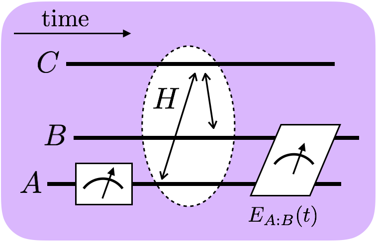
The formal criteria. Consider the scenario depicted in Fig. 1. System is assumed to be the inaccessible object and to mediate the interaction between two remote probes, labeled and . Therefore, from now on, we refer to system as the mediator. It is essential for our method that the probes are not directly coupled and only interact via the mediator. Therefore, the Hamiltonian for the process under scrutiny can be written as , with the interaction Hamiltonian between the mediator and probe . Our work is developed in the context of entanglement distribution with continuous interactions [6]. We first focus on the partition and demonstrate a result which will be instrumental to design our criteria for the inference of non-classicality of based on entanglement dynamics in only. Previous studies on the resources allowing for entanglement distribution showed that any three-body density matrix, i.e. the state of at any time in the present context, satisfies the inequality [7, 8]:
| (1) |
Here is the relative entropy of entanglement in the partition [9], and is the relative entropy of discord [10], also known as the one-way quantum deficit [11]. Note that relative entropy of discord is in general not symmetric, i.e. . Eq. (1) shows that the change in entanglement due to the relocation of is bounded by the quantum discord carried by it.
Let us start from the simple case where the overall probes-mediator system is closed (which allows us to ignore for now the grey-colored shadows in Fig. 1). If the interaction Hamiltonians satisfy , the evolution operator from the initial time to some finite time is just , where and we set . This situation is equivalent to first interacting with and then with (or in reversed order). However, note that the density matrix obtained by “evolving” the initial state through only does not describe the state of the system at . Nevertheless, we now show the relevance of the properties of state for entanglement gain.
Consider the following forms of Eq. (1) written for the initial state and the instrumental state , respectively
| (2) | ||||
Note that , because is local in this partition. The state at time is given by , and thus , this time owing to being local. Summing the above inequalities we obtain a bound on the entanglement gain
| (3) |
This opens up the possibility to create entanglement at time without producing discord at both and , but rather by utilising non-classicality in the instrumental state. In other words, the gain of entanglement in could be mediated by object , which gets non-classically correlated by and then decorrelated by . Therefore, is only classically correlated at times and . We now give a concrete example of this type of entanglement creation.
Consider the interaction Hamiltonian
| (4) |
where is the Pauli- matrix. As initial state we choose the classically correlated state
| (5) |
where e.g. . One can now readily check that the relative entropy of entanglement grows from to in the timespan from to , whereas discord remains zero at these two times. The gain is indeed due to non-classical correlations of the instrumental state: applying only for a time produces discord .
For general non-commuting interaction Hamiltonians, one can pursue a similar analysis with the help of the Suzuki-Trotter expansion. The evolution operator is now discretised into short-time interactions of with and then (or the reversed order) as
| (6) |
where . Accordingly, Eq. (3) holds with replaced by . It is now natural to ask if a scenario exists where entanglement could be increased via interactions with a classical at all times by exploiting the discord in the instrumental state. The example given above is not of this sort because, although we have at and , it is non-zero for . It turns out that, for short evolution times, the discord of the instrumental state cannot be exploited as the following Theorem demonstrates.
Theorem.
For three open systems , , with Hamiltonian and each coupled to its own local environment, the entanglement satisfies the condition if at any time .
Proof.
The proof is presented in Appendix A. ∎
We emphasise the generality of this Theorem, where both mediator and probes are open to their own local environments. This matches a large number of experimentally relevant situations, some of them being addressed in the last part of this paper. The setup where , , and are closed systems is then a special case of the Theorem above in which we have if (see Appendix A). Such Theorem extends the monotonicity of entanglement under local operations and classical communication (LOCC) [12] to the case of continuous interactions. In general, zero-discord states are good models for classical communication as they allow for continuous projective measurements on that do not disturb the whole multipartite state.
We are now in a position to study the presence of discord from observing only. In light of the Theorem above, a promising candidate for this goal is the entanglement gain. However, we now show that some features of the initial tripartite state need to be ensured, but they can be guaranteed by only operating on .
Let us consider Eq. (4) and choose the initial state
| (7) |
where , and and are two Bell states between subsystems . As the initial state in Eq. (7) contains the eigenstates of , the system remains classical, as measured on , at all times. Furthermore, the classical basis is the same at all times. Yet, one can verify that the relative entropy of entanglement between the probes is given by , where is the von Neumann entropy of the state at time , and oscillates between and . Hence, in general, entanglement gain in the partition does not signify the non-classicality of (non-zero ).
Similar considerations have been presented in Ref. [13] to provide a counter-example of the impossibility of entanglement gain via LOCC. However, the partition is entangled already from the beginning (in our example we have ). The subsequent evolution only localises such entanglement to the partition. This example emphasises that the ancillary particles within the framework of LOCC, here , are not allowed to be initially correlated with the principal system, here , even if the correlations are classical.
Furthermore, the only way of gaining entanglement in subsystem via classical is to localise it from the already present entanglement in . This is a consequence of our Theorem and reinforces its role as a proper generalisation of the monotonicity of entanglement to continuous interactions. Namely,
| (8) |
Now, if we ensure by operating on the probes only that the initial entanglements coincide, i.e. , entanglement gain in system is only possible due to non-zero discord . As we are interested in observing entanglement gain, it is natural to start with as small entanglement as possible. This leads us to propose the application of an entanglement-breaking channel to one of the available systems, at time . Indeed, after application of the channel, we have . In a more concrete example, the channel is a von Neumann measurement. An arbitrary measurement is allowed and experimentalist should choose the one having potential for biggest entanglement gain. Note that the measurement results need not be known. Our main detection method is illustrated and summarised in Fig. 2. We stress that entanglement estimation in step (iii) can be realised with entanglement witnesses [14, 15], rendering state tomography unnecessary. (See Appendix B for a criterion based on comparison between entanglement and initial purities of the probes.)
Optomechanics. We address now the practical implications of our criteria for scenarios of current technological relevance. In particular, we consider experiments of cavity optomechanics [16] as the paradigm of an open mesoscopic quantum system for which the criteria identified above hold the potential to be practically significant. In fact, one of the goals of optomechanics is to infer the non-classicality of the state of a massive mechanical system without affecting its (in general fragile) state. A possible setting for such a task is given by a so-called membrane-in-the-middle configuration, where a mechanical oscillator (a membrane) is suspended at the centre of a two-sided optical cavity [17]. By driving the cavity with laser fields from both its input mirrors, respectively, we realise a situation completely analogous to that in Fig. 1 (cf. Fig. 3). We now show that our scheme detects non-classicality of the membrane without measuring it.

The interaction Hamiltonian for the setup in Fig. 3 reads [17]
| (9) |
This is complemented by local terms affecting each subsystem individually (cf. Appendix C). Here and are the annihilation operators for the respective fields, is the dimensionless position-like quadrature of the membrane, and represents the strength of the coupling between field () and the membrane. All the other interactions are local, i.e. () is coupled to its own environment () and is coupled to its thermal phonon reservoir , responsible for the Brownian motion of the membrane. Thus, our Theorem directly applies here and we can implement the detection method of Fig. 2.
In order to independently confirm the non-classicality of the membrane and demonstrate that there is considerable entanglement to be detected we now calculate the ensuing entanglement dynamics. We choose the logarithmic negativity to quantify entanglement. Starting from the experimentally natural state where is in a thermal state and and are coherent states, we calculate the dynamics of and . As initially there is no entanglement, the first step in Fig. 2 can be omitted. The results of our analysis are presented in Fig. 4 for varying power of the right laser. The parameters used in our simulations all adhere to present-day technology [18]. We see that non-zero is always accompanied by non-zero at some time . Note that entanglement is a stronger type of quantum correlations than discord. We have also performed similar calculations by varying the power of the left laser as well as the frequencies of the lasers within experimentally accessible ranges and observed consistent results (see Appendix C).

System-environment correlations. As a second relevant application of our study, let us consider again a closed-system dynamics and, in line with the assumed inaccessibility of the mediator, focus the attention to the probes only. We could thus think of as an environment in contact with the open system . A vast body of literature exists on the study of the influence of initial system-environment correlations (SECs) on the evolution of the open system [19]. Proposals for the detection of SECs based on monitoring the dynamics of distinguishability [20, 21, 22, 23, 24] or purity [25, 26] of the open system have been put forward. Such proposals have been implemented experimentally by means of quantum tomography [27, 28]. Moreover, the possible non-classical nature of SECs was linked to the impossibility of describing the evolution of an open system through completely positive maps [29]. Hence detection schemes of quantum discord in the initial system-environment state have been proposed [30, 31] and recently assessed experimentally [32, 33, 34].
Our scheme of Fig. 2 can also be used to reveal SECs, with the advantage that state tomography is not necessary. This is achieved by dividing the open system into and parts and monitoring the presence of entanglement between them. If one is only interested in the detection of correlations between and , regardless of whether they are classical or not, the entanglement-breaking channel in Fig. 2 can be omitted. Indeed, for the initially uncorrelated state , we have , and no entanglement gain in is possible via classical . Therefore, if one observes a gain, it would either be or at some time. Both cases show correlations between and . Finally, we note that previous schemes detect the non-classicality of the system [30, 31], i.e. presence of , whereas our schemes ascertain the non-classicality of the environment, , which is perhaps a prime example of an inaccessible object.
Other applications. A similar analysis can be done for remote quantum dots in a solid-state substrate [35] or spin-chain systems like in Ref. [36], as their physics also naturally distinguishes a mediating object that is inaccessible, e.g. locations of unpaired spins are unknown in a sample [36]. In a visionary perspective, system could even be a gravitational field coupling massive systems and , which are mutually non-interacting. By determining experimentally the entanglement gain between and one would conclude, according to our scheme, the non-classical nature of the gravitational field between them. That is, if we were to embed into the quantum formalism description of the masses and the field, there would have to be non-orthogonal states in the Hilbert space of the field as this is required for the quantum discord to be non-zero.
Conclusions. We have proposed an entanglement-based criteria for the inference of non-classicality of an inaccessible object. Our protocols are fully non-disruptive of the state of the system to probe, and rely on only weak assumptions on the nature of the interactions involved. They are also robust against decoherence. These features make our proposal suitable to address non-classicality at many levels, from experimentally relevant technological platforms such as quantum optomechanics, to fundamental problems on the nature of gravity.
Acknowledgments. We thank Č. Brukner, K. Modi, M. Piani and A. Winter for stimulating discussions. This work is supported by the National Research Foundation and Singapore Ministry of Education Academic Research Fund Tier 2 project MOE2015-T2-2-034. MP acknowledges support from the EU project TherMiQ, the John Templeton Foundation (grant nr. 43467), the Julian Schwinger Foundation (grant nr. JSF-14-7-0000).
Appendix A Proof of the theorem
Theorem.
For three open systems , , with hamiltonian and each coupled to its own local environment, the entanglement satisfies the condition if at any time .
Proof.
Without loss of generality we take the hamiltonians as and . The same steps can be applied to the general hamiltonians and . As we are assuming vanishing discord (when is measured) at , we can write the initial state as
| (10) |
After a time , the evolved state will be isomorphic to and will read
| (11) |
where both and form orthonormal bases. We assume local environments inducing Markovian dynamics. The evolution can thus be described by the following master equation in Lindblad form (which we write, for convenience, in a coarse-grained time form)
| (12) |
where the last term is the incoherent part of the evolution resulting from interactions with local environments, and we have taken (in light of the declared Lindblad form of the master equation) , where ’s act on system only. We now consider the following conditional state
| (13) | |||||
We go to continuous time by taking , which implies that all terms proportional to can be ignored. Therefore, throughout this proof the symbol “” should be read as “equal up to ”. In this limit, the basis states of can only change as , with orthogonal to and proportional to . This implies that , and thus .
As the commutator in Eq. (13) is multiplied by , the terms in proportional to can already be ignored. One thus finds that
| (14) |
where is the mean energy . Hence the coherent part of the evolution splits into the sum of effective local interactions.
Next, there are three terms for the incoherent part of the evolution. The first two are local in and respectively, and they are proportional to
| (15) |
The last term can be written as
| (16) | |||||
Therefore, we obtain the following explicit form of the conditional state
| (17) | |||||
where we have defined
| (18) | |||||
Accordingly, the state is obtained from by applying Lindblad master equation describing independent local evolutions of subsystems and . The probability can be recovered by noting that the trace of Eq. (17) equals unity. In particular,
| (19) | |||||
where we have used the cyclic property of trace. Note that the numbers multiplying states and in Eq. (17) are all non-negative and sum up to unity, i.e. they form a probability distribution.
Finally, we have
| (20) | |||||
| (21) | |||||
| (22) |
where the involved steps are justified as follows. In the first line we use the flags condition [37]. The inequality follows from applying convexity of the relative entropy of entanglement to and next monotonicity of entanglement under local operations and classical communication . By inserting in between and in the second line of (21) and exchanging dummy indices , one finds that it cancels the third line, giving Eq. (22). In the last step we again use the flags condition, this time to the initial state. The theorem is apparent by evolving the system successively from to and having at anytime . ∎
A special case worth noticing is when the three systems are closed, i.e. we have unitary evolution with hamiltonian . In this case, it follows that the conditional state reads
| (23) |
where . Taking the trace of Eq. (23) gives us and . The conditional state evolves under effective local unitary transformations, hence entanglement in the partition stays the same. By utilising the flags condition as in the proof of the theorem given above, one can show that .
Appendix B A simple criterion based on purity
An elegant criterion for revealing the non-classicality can be derived in terms of the initial purity of probes. Here we take the purity to be given by the von Neumann entropy. Our starting point is Eq. (8) of the main text, which is here repeated for convenience:
| (24) |
We will now bound the initial entanglement by the purity of the probes only. The relative entropy of entanglement is upper bounded by the mutual information [10]. From the sub-additivity of entropy for the subsystem we have , and as the state of is assumed to be classical, , we get . Accordingly,
| (25) |
Any violation of this inequality reveals the non-classicality of , i.e. non-zero at some time during the evolution.
Appendix C Detailed assessment of the optomechanical application
The hamiltonian of the setup (Fig. 3 in the main text) in a rotating frame with frequency of the lasers can be written as where [16]:
| (26) | |||||
and
| (27) |
where the annihilation (creation) operator of field is denoted by () with , and are dimensionless quadratures of the membrane with , is the driving strength of laser with , where is the laser power and denotes its frequency. is decay rate of cavity with finesse . Cavity-laser detuning is defined as , where is the frequency of the cavity and represents field-membrane coupling strength, where is the length of the cavity, is the mass of the membrane and is its natural frequency. Note that is local in partition and the two terms in represent coupling in the partition and respectively.
The dynamics of the operators, adding into account noise and damping terms (also local), can be well written by a set of Langevin equations in Heisenberg picture
| (28) |
where is damping rate of the membrane. Also is input noise of field associated with cavity-input mirror interface and has only correlation function [38], whereas is Brownian noise of the membrane and has correlation function in the limit of interest that is large mechanical quality of the membrane, i.e. [39, 40]. The mean phonon number of the membrane reads .
The linearised Langevin equations can be obtained by splitting the operators into steady state values and fluctuating terms. In particular we write , , and . By inserting these into Eq. (28) and ignoring nonlinear terms and one gets a set of linear Langevin equations for the fluctuation of the quadratures
| (29) |
where effective detuning , , and effective coupling . The steady state values are given by , , and . The quadratures of the field and are related to the field operator through . This relation also applies for the input noise, i.e. .
For simplicity one can re-write Eq. (29) as a single matrix equation where the vector , , and
| (30) |
The solution to linearised Langevin equation is then where .
The quantum state of the fluctuations is fully characterised by covariance matrix . Note that the Gaussian nature of the initial state is maintained since we have linear dynamics and the noises involved are zero-mean Gaussian noises. One can show that the covariance matrix at time is where . A more explicit solution of the covariance matrix, after integration, is given by
| (31) | |||||
which is linear and can easily be solved numerically. As mentioned in the main text we take the initial state to be thermal state for and coherent state for field , this gives . If one is only interested in steady state solution, it is guaranteed when all real parts of eigenvalues of are negative, giving such that the steady state covariance matrix can be calculated from a simpler equation .
The covariance matrix describing our three-mode optomechanical system can be written in block form
| (32) |
where for the block component is a matrix describing local mode correlation when and intermodal correlation when . An -mode covariance matrix has symplectic eigenvalues that can be computed from the spectrum of matrix [41] where
| (33) |
For a physical covariance matrix [42]. For an entangled system, e.g. in the partition , the covariance matrix will not be physical after partial transposition with respect to mode (this is equivalent to flipping the sign of the membrane’s momentum fluctuation operator in ). For our system, this unphysical is shown by one of its three symplectic eigenvalues . Entanglement is then quantified by logarithmic negativity as follows [43, 44]. Note that the separability condition, when has , is sufficient and necessary for mode partition [45]. Entanglement is calculated in similar manner by only considering system where the covariance matrix is now
| (34) |
For our calculations we vary laser power and laser-cavity detuning . Other parameters have been fixed such that this setup is viable with present-day technology [18]. This includes , , , and . Finesse of each cavity is .
The dynamics of entanglement quantified by logarithmic negativity is shown in Fig. 4 in the main text. It is clear that nonzero implies non-classicality of the membrane. If one is interested only in the steady state regime, Fig. 5 shows the corresponding entanglement while is zero in this range (not shown). Note that red colour has been used in the plots for parameters that do not correspond to steady state solution.

References
- [1] L. Henderson and V. Vedral, Classical, quantum and total correlations, J. Phys. A 34, 6899 (2001).
- [2] H. Ollivier and W. H. Zurek, Quantum discord: a measure of the quantumness of correlations, Phys. Rev. Lett. 88, 017901 (2001).
- [3] L. C. Celeri, J. Maziero, and R. M. Serra, Theoretical and experimental aspects of quantum discord and related measures, Int. J. Quant. Inf. 9, 1837 (2011).
- [4] K. Modi, A. Brodutch, H. Cable, T. Paterek, and V. Vedral, The classical-quantum boundary for correlations: discord and related measures, Rev. Mod. Phys. 84, 1655 (2012).
- [5] G. Adesso, T. R. Bromley, and M. Cianciaruso, Measures and applications of quantum correlations, J. Phys. A 49, 473001 (2016).
- [6] T. S. Cubitt, F. Verstraete, W. Dür, and J. I. Cirac, Separable states can be used to distribute entanglement, Phys. Rev. Lett. 91, 037902 (2003).
- [7] A. Streltsov, H. Kampermann, and D. Bruß, Quantum cost for sending entanglement, Phys. Rev. Lett. 108, 250501 (2012).
- [8] T. K. Chuan, J. Maillard, K. Modi, T. Paterek, M. Paternostro, and M. Piani, Quantum discord bounds the amount of distributed entanglement, Phys. Rev. Lett. 109, 070501 (2012).
- [9] V. Vedral, M. B. Plenio, M. A. Rippin, and P. L. Knight, Quantifying entanglement, Phys. Rev. Lett. 78, 2275 (1997).
- [10] K. Modi, T. Paterek, W. Son, V. Vedral, and M. Williamson, Unified view of quantum and classical correlations, Phys. Rev. Lett. 104, 080501 (2010).
- [11] M. Horodecki, P. Horodecki, R. Horodecki, J. Oppenheim, A. Sen, U. Sen, and B. Synak-Radtke, Local versus nonlocal information in quantum-information theory: formalism and phenomena, Phys. Rev. A 71, 062307 (2005).
- [12] C. H. Bennett, D. P. DiVincenzo, J. A. Smolin, and W. K. Wootters, Mixed-state entanglement and quantum error correction, Phys. Rev. A 54, 3824 (1996).
- [13] L. Gyongyosi, The correlation conversion property of quantum channels, Quant. Inf. Proc. 13, 467 (2014).
- [14] M. Horodecki, P. Horodecki, and R. Horodecki, Separability of mixed states: necessary and sufficient conditions, Phys. Lett. A 223, 1 (1996).
- [15] R. Horodecki, P. Horodecki, M. Horodecki, and K. Horodecki, Quantum entanglement, Rev. Mod. Phys. 81, 865 (2009).
- [16] M. Aspelmeyer, T. J. Kippenberg, and F. Marquardt, Cavity optomechanics, Rev. Mod. Phys. 86, 1391 (2014).
- [17] M. Paternostro, D. Vitali, S. Gigan, M. S. Kim, C. Brukner, J. Eisert, and M. Aspelmeyer, Creating and probing multipartite macroscopic entanglement with light, Phys. Rev. Lett. 99, 250401 (2007).
- [18] S. Gröblacher, K. Hammerer, M. R. Vanner, and M. Aspelmeyer, Observation of strong coupling between a micromechanical resonator and an optical cavity field, Nature 460, 724 (2009).
- [19] H. P. Breuer and F. Petruccione, The theory of open quantum systems. (Oxford University Press, 2002).
- [20] E. M. Laine, J. Piilo, and H. P. Breuer, Witness for initial system-environment correlations in open-system dynamics, Europhys. Lett. 92, 60010 (2011).
- [21] A. Smirne, H. P. Breuer, J. Piilo, and B. Vacchini, Initial correlations in open-systems dynamics: the Jaynes-Cummings model, Phys. Rev. A 82, 062114 (2010).
- [22] J. Dajka and J. Łuczka, Distance growth of quantum states due to initial system-environment correlations, Phys. Rev. A 82, 012341 (2010).
- [23] J. Dajka, J. Łuczka, and P. Hänggi, Distance between quantum states in the presence of initial qubit-environment correlations: A comparative study, Phys. Rev. A 84, 032120 (2011).
- [24] S. Wißmann, B. Leggio, and H. P. Breuer, Detecting initial system-environment correlations: Performance of various distance measures for quantum states, Phys. Rev. A 88, 022108 (2013).
- [25] G. Kimura, H. Ohno, and H. Hayashi, How to detect a possible correlation from the information of a subsystem in quantum-mechanical systems, Phys. Rev. A 76, 042123 (2007).
- [26] D. Z. Rossatto, T. Werlang, L. K. Castelano, C. J. Villas-Boas, and F. F. Fanchini, Purity as a witness for initial system-environment correlations in open-system dynamics, Phys. Rev. A 84, 042113 (2011).
- [27] A. Smirne, D. Brivio, S. Cialdi, B. Vacchini, and M. G. A. Paris, Experimental investigation of initial system-environment correlations via trace-distance evolution, Phys. Rev. A 84, 032112 (2011).
- [28] C. F. Li, J. S. Tang, Y. L. Li, and G. C. Guo, Experimentally witnessing the initial correlation between an open quantum system and its environment, Phys. Rev. A 83, 064102 (2011).
- [29] C. A. Rodríguez-Rosario, K. Modi, A. M. Kuah, A. Shaji, and E. C. G. Sudarshan, Completely positive maps and classical correlations, J. Phys. A 41, 205301 (2008).
- [30] M. Gessner and H. P. Breuer, Detecting nonclassical system-environment correlations by local operations, Phys. Rev. Lett. 107, 180402 (2011).
- [31] M. Gessner and H. P. Breuer, Local witness for bipartite quantum discord, Phys. Rev. A 87, 042107 (2013).
- [32] M. Gessner, M. Ramm, T. Pruttivarasin, A. Buchleitner, H. P. Breuer, and H. Häffner, Local detection of quantum correlations with a single trapped ion, Nature Phys. 10, 105 (2014).
- [33] J. S. Tang, Y. T. Wang, G. Chen, Y. Zou, C. F. Li, G. C. Guo, Y. Yu, M. F. Li, G. W. Zha, H. Q. Ni, and Z. C. Niu, Experimental detection of polarization-frequency quantum correlations in a photonic quantum channel by local operations, Optica 2, 1014 (2015).
- [34] S. Cialdi, A. Smirne, M. G. A. Paris, S. Olivares, and B. Vacchini, Two-step procedure to discriminate discordant from classical correlated or factorized states, Phys. Rev. A 90, 050301 (2014).
- [35] T. A. Baart, T. Fujita, C. Reichl, W. Wegscheider, and L. M. K. Vandersypen, Coherent spin-exchange via a quantum mediator, Nature Nanotech. 12, 26 (2017).
- [36] S. Sahling, G. Remeny, C. Paulsen, P. Monceau, V. Saligrama, C. Marin, A. Revcolevschi, L. P. Regnault, S. Raymond, and J. E. Lorenzo, Experimental realization of long-distance entanglement between spins in antiferromagnetic quantum spin chains, Nature Phys. 11, 255 (2015).
- [37] M. Horodecki, Simplifying monotonicity conditions for entanglement measures, Open Sys. Inf. Dyn. 12, 231 (2005).
- [38] D. F. Walls and G. J. Milburn, Quantum optics. (Springer Science & Business Media, 2007).
- [39] V. Giovannetti and D. Vitali, Phase-noise measurement in a cavity with a movable mirror undergoing quantum brownian motion. Phys. Rev. A 63, 023812 (2001).
- [40] R. Benguria and M. Kac, Quantum Langevin equation. Phys. Rev. Lett. 46, 1 (1981).
- [41] C. Weedbrook, S. Pirandola, R. García-Patrón, N. J. Cerf, T. C. Ralph, J. H. Shapiro, and S. Lloyd, Gaussian quantum information. Rev. Mod. Phys. 84, 621 (2012).
- [42] In Ref. [41] the condition is . The absence of the factor of is due to the setting of .
- [43] G. Vidal and R. F. Werner, Computable measure of entanglement. Phys. Rev. A 65, 032314 (2002).
- [44] G. Adesso, A. Serafini, and F. Illuminati, Extremal entanglement and mixedness in continuous variable systems. Phys. Rev. A 70, 022318 (2004).
- [45] R. F. Werner and M. M. Wolf, Bound entangled gaussian states. Phys. Rev. Lett. 86, 3658 (2001).