Approach to Chandrasekhar-Kendall-Woltjer State in a Chiral Plasma
Abstract
We study the time evolution of the magnetic field in a plasma with a chiral magnetic current. The Vector Spherical Harmonic functions (VSH) are used to expand all fields. We define a measure for the Chandrasekhar-Kendall-Woltjer (CKW) state, which has a simple form in VSH expansion. We propose the conditions for a general class of initial momentum spectra that will evolve into the CKW state. For this class of initial conditions, to approach the CKW state, (i) a non-vanishing chiral magnetic conductivity is necessary, and (ii) the time integration of the product of the electric resistivity and chiral magnetic conductivity must grow faster than the time integration of the resistivity. We give a few examples to test these conditions numerically which work very well.
I Introduction
In high energy heavy-ion collisions, two heavy nuclei are accelerated to almost the speed of light and produce very strong electric and magnetic fields at the moment of the collision [1, 2, 3, 4, 5, 6, 7, 8, 9, 10]. The magnitude of magnetic fields can be estimated as , where and are the proton number and the radius of the nucleus respectively, is the the velocity of the nucleus and is the Lorentz contraction factor ( is the nucleon mass and is the collision energy per nucleon). In Au+Au collisions at the Relativistic Heavy Ion Collider (RHIC) with GeV, the peak value of the magnetic field at the moment of the collision is about ( is the pion mass) or Gauss. In Pb+Pb collisions at the Large Hadron Collider (LHC) with TeV, the peak value of the magnetic field can be 10 times as large as at RHIC. Such high magnetic fields enter strong interaction regime and may have observable effects on the hadronic events. The chiral magnetic effect (CME) is one of them which is the generation of an electric current induced by magnetic fields from of the imbalance of chiral fermions [1, 11, 12]. The CME and other related effects have been widely studied in quark-gluon plasma produced in heavy-ion collisions. The charge separation effect observed in STAR [13, 14] and ALICE [15] experiments are consistent to the CME predictions, although there may be other sources such as collective flows that contribute to the charge separation [16]. The CME has recently been confirmed to exist in materials such as Dirac and Weyl semi-metals [17, 18, 19].
In hot and dense matter an imbalance in the number of right-handed quarks and left-handed quarks may be produced through transitions between vacua of different Chern-Simons numbers in some domains of the matter. This is called chiral anomaly and is described by the anomalous conservation law for the axial current,
| (1) |
where denotes the axial 4-vector current with being the chiral charge, and are the number of colors and flavors of quarks respectively, is the electric charge (in the unit of electron charge ) of the quark with flavor , denotes the field strength of the electromagnetic field and is its dual, is the strong coupling constant, denotes the field strength of the -th gluon with and is its dual. The first term on the right-hand-side of Eq. (1) is the anomaly term from electromagnetic fields while the second one is from gluonic fields. In Eq. (1) we have neglected quark masses. For electromagnetic fields we can write in the 3-vector form using , where and are the electric and magnetic 3-vector field respectively.
The axial current breaks the parity locally and may appear in one event, but it is vanishing when taking event average. With such an imbalance, an electric current can be induced along the magnetic field, so the total electric current can be written as
| (2) |
where and are the electric and chiral conductivity respectively. Note that is proportional to the difference between the number of right-handed quarks and left-handed quarks which breaks the parity but conserves the time reversal symmetry. This is in contrast with the electric conductivity which breaks the time reversal symmetry but conserves the parity. So the Ohm’s current is dissipative (with heat production) while the chiral magnetic current is non-dissipative.
We consider a system of charged fermions in electromagnetic fields. The term of or in Eq. (1) is actually related to the magnetic helicity . Then we can take volume integration of Eq. (1) and obtain
| (3) |
where the total helicity is defined by combining the magnetic helicity and the chiral charge ,
| (4) |
where . This means that the magnetic helicity and the chiral charge of fermions can be transferred into each other.
The Chandrasekhar-Kendall-Woltjer (CKW) state is a state of the magnetic field which satisfies the following equation
| (5) |
where is a constant. The CKW state was first studied by Chandrasekhar, Kendall and Woltjer [20, 21, 22, 23] as a force free state. We notice that in a plasma with the chiral magnetic current (2), if the Ohm’s current is absent, the system reaches a special CKW state with following the Ampere’s law. To our knowledge, this idea was first proposed in [24]. But with the Ohm’s current, can the CKW state still be reached? This question can be re-phrased as: what are the conditions under which the CKW state can be reached in a plasma with chiral magnetic currents? In this paper we will answer this question by studying the evolution of magnetic fields with the Maxwell-Chern-Simons equations.
In classical plasma physics, a state satisfying Eq. (5) is called the Taylor state or the Woltjer-Taylor state. It was first found by Woltjer [23] that the CKW state minimizes the magnetic energy for a fixed magnetic helicity. In toroidal plasma devices, such a state is often observed as a self-generated state called reverse field pinch with the distinct feature that the toroidal fields in the center and the edge point to opposite directions. Taylor [25, 26] first argued that the minimization of magnetic energy with a fix magnetic helicity is realized as a selective decay process in a weakly dissipative plasma when the dynamics is dominated by short wavelength structures. Taylor’s theory has been questioned and debated intensely, and alternative theories has been proposed [27, 28]. It is certainly interesting that both classical plasmas and chiral plasmas have the tendency to evolve towards such a state, which suggests that the two systems may share certain dynamics features responsible for the emerging of the state. A brief discussion in this aspect is given in the paper as well.
The paper is organized as follows. In Section II, we start with the Maxwell-Chern-Simons equations and define a global measure for the CKW state by the magnetic field and the electric current. In Section III, we expand all fields in Vector Spherical Harmonic (VSH) functions. The inner products have simple forms in the VSH expansion. The parity of a quantity can be easily identified in the VSH form. We give in Section IV the solution to the Maxwell-Chern-Simons equations for each mode in the VSH expansion. The conditions for the CKW state are given in Section V. In Section VI we test these conditions by examples including the ones with constant and self-consistently determined . We also generalize the momentum spectra at the initial time from a power to a polynomial pre-factor of scalar momentum in Section VII. The summary and conclusions are made in the last section.
II Maxwell-Chern-Simons equations and CKW state
We start from Maxwell-Chern-Simons equations or anomalous Maxwell equations,
| (6) | ||||
| (7) | ||||
| (8) | ||||
| (9) |
where we have included the induced current and neglected the displacement current . We have also dropped the external charge and current density. We assume that and depend on only.
Taking curl of Eq. (6) and using Eqs. (7,8), we obtain
| (10) |
A similar equation for can also be derived but we will not consider it in the current study. To measure whether the CKW state is reached in the evolution of the magnetic field, we introduce the quantity
| (11) |
where we have used the notation for the inner product for any vector field and . According to the Cauchy-Schwartz inequality
| (12) |
we have , where the equality holds only in the case of when the CKW state is reached [28]. We assume that is a smooth function of . The condition that the CKW state is reached can be given by
| (13) |
Note that should not exactly be equal to 1, since is a smooth function of and bounded by the upper limit 1.
To see the time evolution of , it is helpful to write inner products in simple forms, which we will do in the next section.
III Expansion in vector spherical harmonic functions
In this section, we will expand all fields in the basis of Vector Spherical Harmonic function (VSH), with which we can put inner products into a simple and symmetric form.
III.1 Expansion in VSH
The quantities we use to express in Eq. (11) are and . We can extend the series to include more curls,
| (14) |
So the inner products can be written as with and are non-negative integers. To find an unified form for the fields in this series, we can expand in the Coulomb gauge in VSH
| (15) |
where is the scalar momentum and are the quantum number of the angular momentum and the angular momentum along a particular direction respectively. are divergence-free vector fields which can be expressed in term of VSH [29]. The explicit form of can be found in, e.g., Ref. [30, 31]. The orthogonal basis functions satisfy the following orthogonality relations,
| (16) |
where . Note that themselves are CKW states satisfying
| (17) |
and are divergence-free, , so we can expand any divergence-free vector fields in . We note that is real while and are complex.
III.2 Inner products
We can put the general inner products into a simple form by using the orthogonality relation (16),
| (20) |
where are defined by
| (21) |
We note that are positive definite. In deriving Eq. (20) we have used the fact that is real so that . For convenience, we use the following short-hand notation for the integral
| (22) |
From Eq. (20) it is easy to verify
| (23) |
for . This is consistent to the identity . In Table (1), we list the VSH forms of some inner products that we are going to study later in this paper.
| Quantity | VSH form | Short-hand | Parity |
|---|---|---|---|
| even | |||
| odd | |||
| even | |||
| odd |
III.3 Parity and helicity
From Eq. (17), the parity transformation is equivalent to the interchange of the and mode. In the series (14), the quantity is parity-even/parity-odd (P-even/P-odd) for odd/even . For instance, , and are P-odd, P-even and P-odd respectively.
Also the inner product is P-even/P-odd for even/odd , see the last column of Table (1) where the magnetic helicity is P-odd, and the magnetic energy is P-even.
For a momentum spectrum containing only , the helicity is positive. If such a magnetic field can approach the CKW state, it means because is also positive for mode. In contrast it would mean for a momentum spectrum containing only .
IV Solving Maxwell-Chern-Simons equations in VSH
The evolution equation of in (10) can be transformed into equations for or equivalently with Eqs. (19,16),
| (24) |
where is the electric resistivity.
The solution of is in the form
| (25) |
where denote the values at the initial time , and and are defined by
| (26) |
Note that both and are positive.
Alternatively we can rescale time by using as a new evolution parameter, and rewrite , i.e., is the integrated value of from to .
There is a competition between and for approaching or departing the CKW state. Large values of is favored for the CKW state. We will show that it is indeed determined by the increasing ratio of to .
Note that in Eq. (25) changing is equivalent to interchanging the positive and negative modes, therefore we can assume in this paper without loss of generality.
V Conditions for CKW state
In this section we will study the evolution of the fields in the basis of VSH and look for the conditions for the CKW state.
From Eq. (11) we obtain in VSH,
| (27) |
To verify , it is better to rewrite in a more symmetric form,
| (28) |
The difference between the denominator and numerator is
| (29) |
where we have used in the first inequality. From the inequality (29) it is obvious that , where the equality holds for and one of and is zero.
Therefore we have two conditions under which is satisfied:
| (30) |
where is the central momentum of during evolution. Both conditions can be physically understood. The first condition is actually the presence of (we have assumed ), which makes positive modes grow with time while negative modes decay away. It means that the CKW state should contain only positive (or negative) helicity mode only, which is reasonable because the CKW state is the eigenstate of the curl operator. For the second condition, we notice that bases themselves are CKW states from Eq. (17), therefore one single mode in the expansion (19) is natually the CKW state. The authors of Ref. [30] observed in the evolution to the CKW state. However, the delta function is not well defined mathematically, so the second condition is hard to implement and we must find a better one to replace it.
With the solutions for in Eq. (25), we obtain the time behavior of from Eq. (27)
| (31) |
where the time functions are defined by
| (32) |
Here are the powers of in the integrals for , and , respectively.
If the initial spectrum functions contain only ( is a real number), or ( and are real constants), the integrals are just Gaussian-like integrals and easy to deal with. In this paper we assume that take the following form
| (33) |
A typical example of magnetic fields expressed in such a form is the Hopf state [32]. Although this assumption narrows the scope of , it is still general enough: these three kinds of functions are widely used in other fields of physics. It is natural to combine with in the integrand of and re-define the time function as
| (34) |
where is the power of in the initial spectrum functions . Note that does not converge, so we assume . By changing the integral variable where is always positive by definition, we can rewrite in the form
| (35) |
where are defined by
| (36) |
with the time functions by
| (37) |
We rewrite in Eq. (31) as a function of through ,
| (38) |
We give relevant properties of in Appendix A. One property is that are monotonically increasing functions of , which approach zero at , but rise sharply to at . By Eq. (37), if grows faster than with , we have as . As time goes on, associated with positive modes will grow up but associated with negative modes will decay away. At , Eq. (38) becomes
| (39) |
This fulfills the first condition for the CKW state in (30), i.e. only the positive modes survive at the end of the time evolution.
We also show in Appendix A that the right hand side of Eq. (39) tend to 1 if and only if . To make at requires , or
| (40) |
So we can summarize the conditions for the CKW state to be reached in time evolution:
| (41) |
Note that or plays an essential role: it makes negative modes more and more suppressed while making positive modes blow up as time goes on. At the same time it makes at so that .
In heavy-ion collisions, and are decreasing functions of as the result of the expansion of the QGP matter. It is natural to assume that and fall with time in power laws [33], and , where . This can be justified by the fact that MeV [34] and [35], where both the temperature and the chiral chemical potential decrease with time in power laws in expansion. In this case we have , following Eq. (26), and , the condition for the CKW state now becomes
| (42) |
The above condition is very easy to check and it is one of the most useful and practical criteria in this paper.
The fact that a large will bring the system to the CKW state shows that a non-Ohmic current may play a crucial role in the process of reaching the CKW state. This suggests that in classical plasmas systems, a non-Ohmic current, e.g., the Hall current, could produce the same effect. In a classical system with the Hall current and negligible flow velocity, the evolution of the magnetic field is governed by
| (43) |
where is the density of the plasma, is electron charge, and the last is the Hall current term. Obviously, with a small resistivity, the system approaches equilibrium when the CKW state is reached.
VI Examples and tests of conditions
In this section we will look at examples of the CKW state to test the conditions we propose in the last section.
VI.1 With only
As the first example, let us consider an initial spectrum with only without . We assume has the following form,
| (44) |
where characterizes the length scale of the magnetic field, is the initial magnetic helicity. The normalization constant is chosen to be which gives the initial magnetic helicity of the spectrum,
| (45) |
From Eq. (39) we obtain
| (46) |
where
| (47) |
is given by Eq. (37) with and . Here we have suppressed the superscript of and simply denote .
To verify our conditions for the CKW state, we consider following cases:
| a) | ||||
| b) | ||||
| c) | ||||
| d) | (48) |
In case a) both and are constants, which is used in Refs. [9, 10] to calculate the magnetic field in medium. In this case, we have and in late time which satisfies the condition , and we can see the effect of non-vanishing constant . Such an effect can be seen by comparing with case b) in which we switch off . In case c) is still a constant as same as case a), but is chosen to break the condition with and . In case d), the values and are used in Refs. [33, 36], which are thought to be more reasonable in heavy-ion collisions. But we note that in real situations of heavy-ion collisions, the time behaviors of and can be very complicated (may not follow power laws), but our conditions in (41) are still applicable.
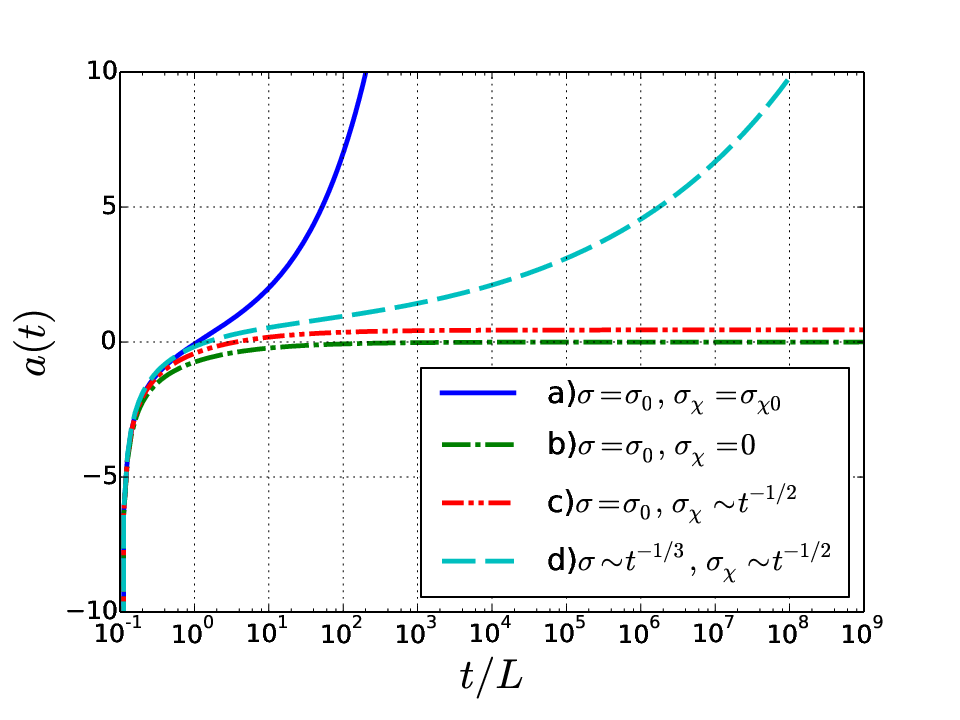

For numerical simulation, we choose and . The results are shown in Fig. 1. Indeed in case a) and d), the CKW state can be reached. As goes from to , according to Eqs. (46, 47, 66), evolves from to , and evolves from 0.8 to 1. In case b) and c) the condition (42) is not satisfied, the CKW state is inaccessible. Indeed the simulation shows that it is true since tends toward 0 and in case b) and c) at , respectively. Even though and increase with , we have and at corresponding to and respectively. All these results show that the conditions work well.
But we should point out that constant and or even the power law decayed and may not be physical since once persists for a long time, growing faster than will make some physical quantities diverge. We look at the magnetic helicity and the magnetic energy ,
| (49) |
The numerical results of the magnetic helicity are shown in Fig. 2. The results of the magnetic energy are similar. In case b) and c), since and converge to constants, but keeps growing, both and finally decay to zero following Eq. (49). However in case a) and d), and increase to in late time, and from Eq (65) grow much faster than to make and blow up.

From Eq. (24), we see that the spectrum grows exponentially in time for , such an instability has been discussed in [9, 37], see also [38]. This instability is the source of the divergence of and . Such an unphysical inflation can be understood: the appearance of in the induced current leads to the positive feedback that the magnetic field itself induces the magnetic field. If we put no constraint on , as the result, the magnetic field will keep growing and finally blow up at some time. This of course breaks conservation laws. One way to avoid such divergences is to implement conservation laws in the system. This is the topic of the next subsection.
VI.2 With only and dynamical
We now consider imposing the total helicity conservation in Eq. (4). This has been implemented in Ref. [37, 30]. Here we focus on the approach to the CKW state in evolution. For simplicity, we can parameterize as
| (50) |
where and (total helicity) are constants. From Eq. (50), we see that the requirement leads to . The initial spectrum is assumed to be the same as Eq. (44), so we have . The parameters are chosen to be , , and , where is given by Eq. (45). Since is a constant, we have . We can solve self-consistently through ,
| (51) |
where we have used and that depends on through in Eq. (49).

The numerical results for , and are presented in Fig. 3. For comparison, we also show the result for constant with . In both cases, at the beginning, is not large enough to make grows faster than , which makes in Eq. (49) decrease with time. After grows large enough as time goes on, starts to increase after reaching a minimum. In the case of dynamical , according to Eq. (50), and are complementary to each other to make up a seesaw system. In this system, the decreasing of at the beginning raises the value of and makes and grow faster. As the result, the turning point comes earlier than the case of constant . As keeps growing, drops down leading to slower increase of , which makes grows slower. At the end, is saturated to instead of blowing up.
Let us look at the asymptotic time behavior of as . As the magnetic helicity is saturated to following Eq. (49), with and at late time, we obtain
| (52) |
where and is called product logarithm, which is the inverse function of . From , we obtain at very large ,
| (53) |
Since the term increases with , is always growing faster than . Thus the conditions are satisfied and the CKW state can be reached.
Taking a derivative of with respect to , we obtain at late time from Eq. (53),
| (54) |
The asymptotic behavior of is which decays slower than . We show the result from Eq. (54) in the black short dashed line in Fig. 3, which agrees with the numerical result very well.
We have also looked at a general spectrum for at initial time,
| (55) |
where the normalization constant is determined by the initial magnetic helicity . We assume obeying the power law decay in time, which gives . In this case, solving Eq. (51) gives the late time asymptotic behavior,
| (56) |
Again we see that grows faster than and the CKW state can be finally reached.
VI.3 With mixed helicity
In this example we consider both positive and negative modes. We will show that only the positive mode survives while the negative mode decays away in late time. Let us consider the most extreme case in which the initial spectra of the positive and negative modes are the same. We take the following initial spectra for ,
| (57) |
It is obvious that the initial magnetic helicity is zero. Since , is given by Eq. (38) with and . Obviously at the initial time we have because .
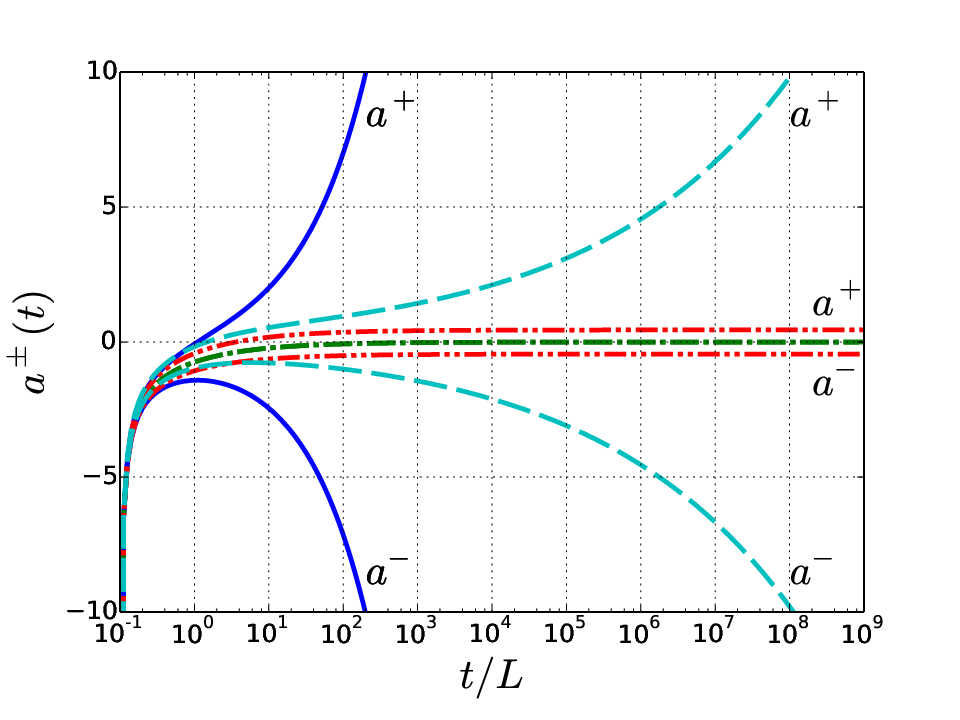
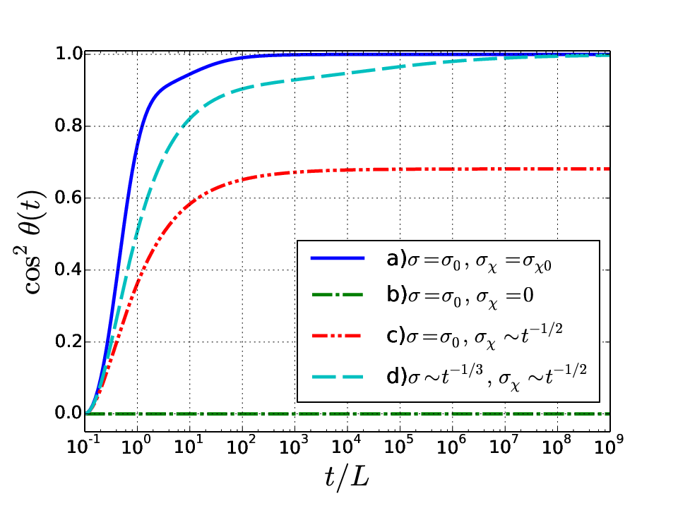
We consider again the cases a)-d) as in (48). The results are shown in Fig. 4. The CKW state can be approached in case a) and d). As is shown in the left panel of Fig. 4, grow to respectively, therefore at very late time the negative mode becomes highly suppressed and the positive mode survives, leading to approach 1. However in case b) we have and in late time. In this case the negative/positive modes are identical in the time evolution, which results in . In case c) we have which breaks the conditions for the CKW state. In this case, do not go to at , instead they approach the limits . We see that keeps growing with time till it gets saturation, . All these results are consistent with our expectations.
VII More general momentum spectra
The power pre-factor of initial momentum spectra in (33) can be generalized to a polynomial,
| (58) |
where for any due to the fact that must be positive. Here are real numbers with . Ignoring negative modes, we obtain from Eq. (39),
| (59) |
where . According to Eq. (65), the -th term is dominant at , while the -th term is dominant at . We can prove that in Eq. (59) tends toward at by Eq. (66). From Eq. (68), at large positive the ratio can be approximated by . Hence the right-hand-side of Eq. (59) dominated by is also approximately at large positive and reaches 1 for . So our conditions for the CKW state are applicable to the initial momentum spectrum (58) with a polynomial pre-factor.
As examples we consider following initial momentum spectra , and . We compare them with the power pre-factor we considered in the last section. We use Eq. (59) for . In all these cases we have and .

We plot as functions of in Fig. 5. The results show that at , all curves are near 0.8 which implies the -th term is dominant. For moderate values of , the curves for different initial momentum spectra diverge significantly. At large positive , they converge again and approach as expected.
VIII Summary and conclusions
We investigate the Chandrasekhar-Kendall-Woltjer (CKW) state in a plasma with currents induced by chiral anomaly in magnetic fields. We solve the Maxwell-Chern-Simons equations and propose the conditions at which the CKW state can be finally realized in time evolution. We decompose the vector potential and the magnetic field into vector spherical harmonic modes. These modes are labeled by scalar momentum , quantum numbers of orbital angluar momentum and angular momentum along specific direction , and the photon (electromagnetic field) helicity . For each mode, there is an ordinary differential equation in time whose solution can be easily found.
We define a quantity for the CKW state, where can be regarded as the average angle between and . If , the CKW state is reached. In the real world the CKW state cannot be exactly reached but only be approached asymptotically, i.e. . In the bases of vector spherical harmonic functions, a general inner product of two vector fields can be put into a uniform integral, from which we can express in a simple form.
We propose the conditions that the CKW state can be reached in time evolution for a general class of initial momentum spectra: (i) the presence of and (ii) grows faster in time than , where and are integrations over of and of respectively.
We take some examples to test these conditions. The numerical results agree with these conditions very well. In numerical calculations, we set different values for the parameters , , , , and the powers of in initial momentum spectra. We find that in cases of constant and some power law decaying functions, although the CKW state can be approached but the magnetic helicity and magnetic energy will blow up. Such a problem can be avoided with dynamical determined self-consistently with a helicity bound and a negative feedback. The critical decaying behavior of given in Eq. (54) is found both numerically and analytically. The CKW state can be reached at the end of time evolution.
Acknowledgments. QW and XLX thank H. Li and Y.G. Yang for helpful discussions. QW is supported in part by the Major State Basic Research Development Program (MSBRD) in China under Grant 2015CB856902 and 2014CB845402 respectively and by the National Natural Science Foundation of China (NSFC) under the Grant 11535012.
Appendix A Properties of function
We give some useful properties of the function in Eq. (36). For convenience we simply denote this function as in this appendix. We formally define as
| (60) |
where is any real number larger than .
By definition can be integrated as
| (61) |
where is the gamma function and is the confluent hypergeometric function of the first kind. The above formula is applicable for any real number . For being integer, can also be determined recursively by
| (62) |
with
| (63) |
where is the complementary error function, .
From the definition Eq. (60), it is straightforward to have
| (64) |
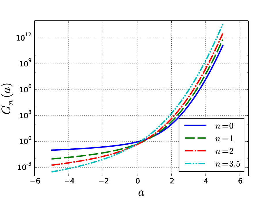
Since are always positive, are monotonically increasing functions of . We plot in Fig. 6 for being integers and a real number as examples. They all approach zero at , but rise sharply to at .

For the purpose of this paper, we are concerned with the asymptotic behavior of at . From Eq. (61) we have found that
| (65) |
This means approach and at respectively, and implies that
| (66) |
We plot the quantity in Fig. 6 for . It shows that they increase with in S-shape from to 1 in the range .
To obtain the asymptote of at , we expand for large to the next to leading order in ,
| (67) |
So the asymptote of the the ratio is
| (68) |
Fig. 6 shows that all the quantity approach the asymptote for large . We see with the larger , they deviate the asymptote further. At very large , they fit very well. We also see tend toward 1 if and only if .
References
- [1] D. E. Kharzeev, L. D. McLerran, and H. J. Warringa, Nucl. Phys. A803, 227 (2008), eprint 0711.0950.
- [2] V. Skokov, A. Yu. Illarionov, and V. Toneev, Int. J. Mod. Phys. A24, 5925 (2009), eprint 0907.1396.
- [3] V. Voronyuk, V. D. Toneev, W. Cassing, E. L. Bratkovskaya, V. P. Konchakovski, and S. A. Voloshin, Phys. Rev. C83, 054911 (2011), eprint 1103.4239.
- [4] W.-T. Deng and X.-G. Huang, Phys. Rev. C85, 044907 (2012), eprint 1201.5108.
- [5] J. Bloczynski, X.-G. Huang, X. Zhang, and J. Liao, Phys. Lett. B718, 1529 (2013), eprint 1209.6594.
- [6] L. McLerran and V. Skokov, Nucl. Phys. A929, 184 (2014), eprint 1305.0774.
- [7] U. Gursoy, D. Kharzeev, and K. Rajagopal, Phys. Rev. C89, 054905 (2014), eprint 1401.3805.
- [8] V. Roy and S. Pu, Phys. Rev. C92, 064902 (2015), eprint 1508.03761.
- [9] K. Tuchin, Phys. Rev. C91, 064902 (2015), eprint 1411.1363.
- [10] H. Li, X.-l. Sheng, and Q. Wang (2016a), eprint 1602.02223.
- [11] K. Fukushima, D. E. Kharzeev, and H. J. Warringa, Phys. Rev. D78, 074033 (2008), eprint 0808.3382.
- [12] D. E. Kharzeev, J. Liao, S. A. Voloshin, and G. Wang, Prog. Part. Nucl. Phys. 88, 1 (2016), eprint 1511.04050.
- [13] B. I. Abelev et al. (STAR), Phys. Rev. Lett. 103, 251601 (2009), eprint 0909.1739.
- [14] B. I. Abelev et al. (STAR), Phys. Rev. C81, 054908 (2010), eprint 0909.1717.
- [15] B. Abelev et al. (ALICE), Phys. Rev. Lett. 110, 012301 (2013), eprint 1207.0900.
- [16] X.-G. Huang, Y. Yin, and J. Liao, in 25th International Conference on Ultra-Relativistic Nucleus-Nucleus Collisions (Quark Matter 2015) Kobe, Japan, September 27-October 3, 2015 (2015), eprint 1512.06602, URL https://inspirehep.net/record/1410880/files/arXiv:1512.06602.pdf.
- [17] D. T. Son and B. Z. Spivak, Phys. Rev. B88, 104412 (2013), eprint 1206.1627.
- [18] G. Basar, D. E. Kharzeev, and H.-U. Yee, Phys. Rev. B89, 035142 (2014), eprint 1305.6338.
- [19] Q. Li, D. E. Kharzeev, C. Zhang, Y. Huang, I. Pletikosic, A. V. Fedorov, R. D. Zhong, J. A. Schneeloch, G. D. Gu, and T. Valla, Nature Phys. 12, 550 (2016b), eprint 1412.6543.
- [20] S. Chandrasekhar, Proceedings of the National Academy of Sciences 42, 1 (1956).
- [21] S. Chandrasekhar and P. Kendall, The Astrophysical Journal 126, 457 (1957).
- [22] S. Chandrasekhar and L. Woltjer, Proceedings of the National Academy of Sciences 44, 285 (1958).
- [23] L. Woltjer, Proceedings of the National Academy of Sciences 44, 489 (1958).
- [24] M. N. Chernodub (2010), eprint 1002.1473.
- [25] J. B. Taylor, Phys. Rev. Lett. 33, 1139 (1974).
- [26] J. B. Taylor, Reviews of Modern Physics 58, 741 (1986).
- [27] S. Ortolani and D. D. Schnack, Magnetohydrodynamics of Plasma Relaxation (World Scientific, Singapore, 1993), p. 56.
- [28] H. Qin, W. Liu, H. Li, and J. Squire, Phy. Rev. Lett. 109, 235001 (2012).
- [29] J. D. Jackson, Classical electrodynamics (Wiley, 1999).
- [30] Y. Hirono, D. Kharzeev, and Y. Yin, Phys. Rev. D92, 125031 (2015), eprint 1509.07790.
- [31] K. Tuchin, Phys. Rev. C93, 054903 (2016), eprint 1601.05399.
- [32] W. T. Irvine and D. Bouwmeester, Nature Physics 4, 716 (2008).
- [33] K. Tuchin, Adv. High Energy Phys. 2013, 490495 (2013), eprint 1301.0099.
- [34] H. T. Ding, A. Francis, O. Kaczmarek, F. Karsch, E. Laermann, and W. Soeldner, Phys. Rev. D83, 034504 (2011), eprint 1012.4963.
- [35] D. E. Kharzeev and H. J. Warringa, Phys. Rev. D80, 034028 (2009), eprint 0907.5007.
- [36] N. Yamamoto, Phys. Rev. D93, 125016 (2016), eprint 1603.08864.
- [37] C. Manuel and J. M. Torres-Rincon, Phys. Rev. D92, 074018 (2015), eprint 1501.07608.
- [38] Y. Akamatsu and N. Yamamoto, Phys. Rev. Lett. 111, 052002 (2013), eprint 1302.2125.