跳到论文正文
W Papers独立论文阅读器 arXiv:1607.01048 论文正文 计算阅读时间 · 0%
引用这篇论文根据当前论文元数据生成,正式投稿前建议核对。


License: arXiv.org perpetual non-exclusive license
arXiv:1607.01048v2 [cs.IT] 10 Feb 2017

Capacity of Gaussian Many-Access ChannelsThanks: X. Chen was with the Department of Electrical Engineering and Computer Science, Northwestern University, Evanston, IL. He is now with Apple Inc., Cupertino, CA. T.-Y. Chen was with the Department of Electrical Engineering and Computer Science, Northwestern University, Evanston, IL. He is now with SpiderCloud Wireless Inc., San Jose, CA. D. Guo is with the Department of Electrical Engineering and Computer Science, Northwestern University, Evanston, IL. dGuo@Northwestern.edu. This work was presented in part at the 2013 IEEE Information Theory Workshop, Sevilla, Spain [1] and the 2014 IEEE International Symposium on Information Theory, Honolulu, HI [2]. This work was supported in part by the National Science Foundation under Grant Nos. ECCS-1231828 and CCF-1423040.

Xu Chen, Tsung-Yi Chen, and Dongning Guo Affiliation: 
Abstract

Classical multiuser information theory studies the fundamental limits of models with a fixed (often small) number of users as the coding blocklength goes to infinity. This work proposes a new paradigm, referred to as many-user information theory, where the number of users is allowed to grow with the blocklength. This paradigm is motivated by emerging systems with a massive number of users in an area, such as the Internet of Things. The focus of the current paper is the many-access channel model, which consists of a single receiver and many transmitters, whose number increases unboundedly with the blocklength. Moreover, an unknown subset of transmitters may transmit in a given block and need to be identified as well as decoded by the receiver. A new notion of capacity is introduced and characterized for the Gaussian many-access channel with random user activities. The capacity can be achieved by first detecting the set of active users and then decoding their messages. The minimum cost of identifying the active users is also quantified.

I Introduction

Classical information theory characterizes the fundamental limits of communication systems by studying the asymptotic regime of infinite coding blocklength. The prevailing models in multiuser information theory assume a fixed (usually small) number of users, where fundamental limits as the coding blocklength goes to infinity are studied. Even in the large-system analysis of multiuser systems [3, 4, 5], the blocklength is sent to infinity before the number of users is sent to infinity.11 1 The same can be said of the many-user broadcast coding strategy for the point-to-point channel proposed in [6], and the CEO problem [7]. In some sensor networks and emerging Internet of Things, a massive and ever-increasing number of wireless devices with sporadic traffic may need to share the spectrum in a given area. This motivates us to rethink the assumption of fixed population of fully buffered users. Here we propose a new many-user paradigm, where the number of users is allowed to increase without bound with the blocklength.22 2 The only existing model of this nature is found in [8], in which the authors sought for uniquely-decodable codes for a noiseless binary adder channel where the number of users increases with the blocklength.

In this paper, we introduce the many-access channel (MnAC) to model systems consisting of a single receiver and many transmitters, the number of which is comparable to or even larger than the blocklength [1, 2]. We study the asymptotic regime where the number of transmitting devices (kk) increases as the blocklength (nn) tends to infinity. The model also accommodates random access, namely, it allows each transmitter to be active with certain probability in each block. We assume synchronous transmission in the model.33 3 A recent follow-up work [9] has studied the capacity of strong asynchronous MnACs.

In general, the classical theory does not apply to systems where the number of users is comparable or larger than the blocklength, such as in a machine-to-machine communication system with many thousands of devices in a given cell. One key reason is that, for many functions of two variables ff, limk→∞limn→∞f⁡(k,n)≠limn→∞f⁡(kn,n)\lim_{k\to\infty}\lim_{n\to\infty}f(k,n)\neq\lim_{n\to\infty}f(k_{n},n), i.e., letting k→∞k\to\infty after n→∞n\to\infty may yield a different result than letting nn and k=knk=k_{n} (as a function of nn) simultaneously tend to infinity. Moreover, the traditional notion of rate in bits per channel use is ill-suited for the task in the many-user regime as noted (for the Gaussian multiaccess channel) in [10, pp. 546–547] by Cover and Thomas, “when the total number of senders is very large, so that there is a lot of interference, we can still send a total amount of information that is arbitrary large even though the rate per individual sender goes to 0.”

Capacity of the conventional multiaccess channel is well understood [11, 12, 13]. The achievable error exponent and capacity region of a random multiaccess channel were derived in [14]. Packet-based random multiaccess communication systems with collision detection have also been studied from the perspective of information theory in [15, 16]. The capacity of the conventional multiaccess channel can be established using the fact that joint typicality is satisfied with probability 1 as the blocklength grows to infinity. This argument, however, does not directly apply to models where the number of users also goes to infinity. Specifically, joint typicality requires the simultaneous convergence of the empirical joint entropy of every subset of the input and output random variables to the corresponding joint entropy. Even though convergence holds for every subset due to the law of large numbers, the asymptotic equipartition property is not guaranteed because the number of those subsets increases exponentially with the number of users [17]. Resorting to strong typicality does not resolve this because the empirical distribution over an increasing alphabet (due to increasing number of users) does not converge.

In general, the received signal of the Gaussian MnAC is a noisy superposition of the codewords chosen by the active users from their respective codebooks. The detection problem boils down to identifying codewords based on their superposition. It is closely related to sparse recovery, also known as compressed sensing, which has been studied in a large body of works [18, 19, 20, 21, 22, 23, 24, 25, 26, 27]. Information-theoretic limits of exact support recovery was considered in [21], and stronger necessary and sufficient conditions have been derived subsequently [23, 24, 27]. Using existing results in the sparse recovery literature, it can be shown that the message length (in bits) that can be transmitted reliably by each user through the MnAC should be in the order of Θ⁡(n⁡(log⁡kn)/kn)\Theta(n(\log k_{n})/k_{n}).

In this paper, we provide a sharp characterization of the capacity of Gaussian many-access channels as well as the user identification cost. As an achievable scheme, each user’s transmission consists of a signature that identifies the user, followed by a message-bearing codeword. The decoder first identifies the set of active users based on the superposition of their unique signatures. (This is in fact a compressed sensing problem [28, 29].) It then decodes the messages from the identified active users. The length of the signature matches the capacity penalty due to user activity uncertainty. The proof techniques find their roots in Gallager’s error exponent analysis [30]. Also studied is a more general setup where groups of users have heterogeneous channel gains and activity patterns. Again, separate identification and decoding is shown to achieve the capacity region. While the exact capacity of the MnAC with given large finite user population and blocklength remains a hard open problem, this paper offers a new asymptotic theory that has a better explanatory power for random massive access than the classical theory.

Unless otherwise noted, we use the following notational conventions: xx denotes a scalar, 𝒙{\boldsymbol{x}} denotes a column vector, and 𝒙¯{\underline{\boldsymbol{x}}} denotes a matrix. The corresponding uppercase letters XX, 𝑿{\boldsymbol{X}}, and 𝑿¯{\underline{\boldsymbol{X}}} denote the corresponding random scalar, random vector and random matrix, respectively. Given a set AA, let 𝒙A=(xi)i∈A{\boldsymbol{x}}_{A}=(x_{i})_{i\in A} denote the subset of variables of 𝒙{\boldsymbol{x}} whose indices are in AA and let 𝒙¯A=(𝒙i)i∈A{\underline{\boldsymbol{x}}}_{A}=({\boldsymbol{x}}_{i})_{i\in A} be the matrix formed by columns of 𝒙¯{\underline{\boldsymbol{x}}} whose indices are in AA. Let xn≤nynx_{n}\leq_{n}y_{n} denote lim supn→∞(xn−yn)≤0\limsup_{n\to\infty}(x_{n}-y_{n})\leq 0. That is, xnx_{n} is essentially asymptotically dominated by yny_{n}. All logarithms are natural. The binary entropy function is denoted as H2​(p)=−p​log⁡p−(1−p)​log⁡(1−p)H_{2}(p)=-p\log p-(1-p)\log(1-p).

The rest of this paper is organized as follows. Section II presents the system model and main results. Section III proves the converse part of the MnAC capacity result. Section IV quantifies the user identification cost. Section V proves the achievability part of the MnAC capacity result. Section VI discusses successive decoding techniques for MnAC. Section VII analyzes the capacity of MnAC with heterogeneous user groups. Concluding remarks are given in Section VIII.

II System Model and Main Results

Let nn denote the number of channel uses, i.e., the blocklength. Let the total number of users be tied to the blocklength and be denoted as ℓn\ell_{n}, which is a function of nn. The received symbols in a block form a column vector of length nn:

𝒀=∑k=1ℓn𝑺k​(wk)+𝒁\displaystyle{\boldsymbol{Y}}=\sum_{k=1}^{\ell_{n}}{\boldsymbol{S}}_{k}(w_{k})+{\boldsymbol{Z}} (1)

where wkw_{k} is the message of user kk, 𝑺k​(wk)∈ℝn{\boldsymbol{S}}_{k}(w_{k})\in\mathbb{R}^{n} is the corresponding nn-symbol codeword, and 𝒁{\boldsymbol{Z}} is a Gaussian noise vector with independent standard Gaussian entries. Suppose each user accesses the channel independently with identical probability αn\alpha_{n} during any given block. If user kk is inactive, it is thought of as transmitting the all-zero codeword 𝒔k​(0)=𝟎{\boldsymbol{s}}_{k}(0)=\mathbf{0}.

Definition 1

Let 𝒮k\mathcal{S}_{k} and 𝒴\mathcal{Y} denote the input alphabet of user kk and the output alphabet of the MnAC, respectively. An (M,n)(M,n) symmetric code with power constraint PP for the MnAC channel (𝒮1×𝒮2×⋯×𝒮ℓn,pY|S1,⋯,Sℓn,𝒴)(\mathcal{S}_{1}\times\mathcal{S}_{2}\times\cdots\times\mathcal{S}_{\ell_{n}},p_{Y|S_{1},\cdots,S_{\ell_{n}}},\mathcal{Y}) consists of the following mappings:

  1. 1.

    The encoding functions ℰk:{0,1,…,M}→𝒮kn\mathcal{E}_{k}:\{0,1,\dots,M\}\rightarrow\mathcal{S}_{k}^{n} for every user k∈{1,⋯,ℓn}k\in\{1,\cdots,\ell_{n}\}, which maps any message ww to the codeword 𝒔k​(w)=[sk​1​(w),⋯,sk​n​(w)]T{\boldsymbol{s}}_{k}(w)=[s_{k1}(w),\cdots,s_{kn}(w)]^{T}. In particular, 𝒔k​(0)=𝟎{\boldsymbol{s}}_{k}(0)=\mathbf{0}, for every kk. Every codeword 𝒔k​(w){\boldsymbol{s}}_{k}(w) satisfies the power constraint:

    1n​∑i=1nsk​i2​(w)≤P.\displaystyle\frac{1}{n}\sum_{i=1}^{n}s_{ki}^{2}(w)\leq P. (2)
  2. 2.

    Decoding function 𝒟:𝒴n→{0,1,…,M}ℓn\mathcal{D}:\mathcal{Y}^{n}\rightarrow\{0,1,\dots,M\}^{\ell_{n}}, which is a deterministic rule assigning a decision on the messages to each possible received vector.

The average error probability of the (M,n)(M,n) code is:

𝖯e(n)=𝖯{𝒟(𝒀)≠(W1,…,Wℓn)},\displaystyle\mathsf{P}_{e}^{(n)}=\mathsf{P}\left\{\mathcal{D}({\boldsymbol{Y}})\neq(W_{1},\dots,W_{\ell_{n}})\right\}, (3)

where the messages W1,⋯,WℓnW_{1},\cdots,W_{\ell_{n}} are independent, and for k∈{1,⋯,ℓn}k\in\{1,\cdots,\ell_{n}\}, the message’s distribution is

𝖯{Wk=w}={1−αn,w=0,αnM,w∈{1,…,M}.\displaystyle\mathsf{P}\left\{W_{k}=w\right\}=\begin{cases}1-\alpha_{n},\quad&w=0,\\ \frac{\alpha_{n}}{M},\quad&w\in\{1,\dots,M\}.\end{cases} (4)

The code is said to be symmetric because the message length is the same for all users. (We extend to an asymmetric case in Section VII.) The preceding model reduces to the conventional ℓ\ell-user multiaccess channel in the special case where ℓn=ℓ\ell_{n}=\ell is fixed and αn=1\alpha_{n}=1 as the blocklength nn varies.

II-A The Message-Length Capacity

Definition 2 (Asymptotically achievable message length)

We say a positive nondecreasing sequence of message lengths {v⁡(n)}n=1∞\left\{v(n)\right\}_{n=1}^{\infty}, or simply, v⁡(⋅)v(\cdot), is asymptotically achievable for the MnAC if there exists a sequence of (⌈exp⁡(v⁡(n))⌉,n)(\lceil\exp(v(n))\rceil,n) codes according to Definition 1 such that the average error probability 𝖯e(n)\mathsf{P}_{e}^{(n)} given by (3) vanishes as n→∞n\to\infty.

It should be clear that by asymptotically achievable message length we really mean a function of the blocklength. The base of exp⁡(⋅)\exp(\cdot) should be consistent with the unit of the message length. If the base of exp⁡(⋅)\exp(\cdot) is 2 (resp. ee), then the message length is measured in bits (resp. nats).

Definition 3 (Symmetric message-length capacity)

For the MnAC channel described by (1), a positive nondecreasing function B⁡(n)B(n) of the blocklength nn is said to be a symmetric message-length capacity of the MnAC channel if, for any 0<ϵ<10<\epsilon<1, (1−ϵ)​B​(n)(1-\epsilon)B(n) is an asymptotically achievable message length according to Definition 2, whereas (1+ϵ)​B​(n)(1+\epsilon)B(n) is not asymptotically achievable.

For the special case of a (conventional) multiaccess channel, the symmetric capacity B⁡(n)B(n) in Definition 3 is asymptotically linear in nn, so that limn→∞B⁡(n)/n\lim_{n\to\infty}B(n)/n is equal to the symmetric capacity of the multiaccess channel (in, e.g., bits per channel use). From this point on, by “capacity” we mean the message-length capacity in contrast to the conventional capacity.

Definition 3 is only concerned with the asymptotics of the message length. If B⁡(n)B(n) is a capacity, then so is B⁡(n)+o⁡(B⁡(n))B(n)+o(B(n)). Hence the capacity expression is not unique. In general, the message-length capacity B⁡(n)B(n) need not grow linearly with the blocklength.

Let 𝑺¯k=[𝑺k​(1),⋯,𝑺k​(M)]{\underline{\boldsymbol{S}}}_{k}=[{\boldsymbol{S}}_{k}(1),\cdots,{\boldsymbol{S}}_{k}(M)] denote the matrix consisting of all but the first all-zero codeword of user kk. Let 𝑺¯=[𝑺¯1,⋯,𝑺¯ℓn]∈ℝn×(M​ℓn){\underline{\boldsymbol{S}}}=[{\underline{\boldsymbol{S}}}_{1},\cdots,{\underline{\boldsymbol{S}}}_{\ell_{n}}]\in\mathbb{R}^{n\times(M\ell_{n})} denote the concatenation of the codebooks of all users. For ease of analysis, we often use the following equivalent model for the Gaussian MnAC (1):

𝒀=𝑺¯​𝑿+𝒁,\displaystyle{\boldsymbol{Y}}={\underline{\boldsymbol{S}}}{\boldsymbol{X}}+{\boldsymbol{Z}}, (5)

where 𝒁{\boldsymbol{Z}} is defined as in (1) and 𝑿∈ℝM​ℓn{\boldsymbol{X}}\in\mathbb{R}^{M\ell_{n}} is a vector indicating the codewords transmitted by the users. Specifically, 𝑿=[𝑿1T,𝑿2T,⋯,𝑿ℓnT]T{\boldsymbol{X}}=[{\boldsymbol{X}}_{1}^{T},{\boldsymbol{X}}_{2}^{T},\cdots,{\boldsymbol{X}}_{\ell_{n}}^{T}]^{T}, where 𝑿k∈ℝM{\boldsymbol{X}}_{k}\in\mathbb{R}^{M} indicates the codeword transmitted by user kk, k=1,⋯,ℓnk=1,\cdots,\ell_{n}, i.e.,

𝑿k={𝟎 with probability ​1−αn𝒆m with probability ​αnM,m=1,…,M\displaystyle{\boldsymbol{X}}_{k}=\begin{cases}\mathbf{0}\;\;&\text{ with probability }1-\alpha_{n}\\ {\boldsymbol{e}}_{m}&\text{ with probability }\frac{\alpha_{n}}{M},\enskip m=1,\dots,M\end{cases} (6)

where 𝒆m{\boldsymbol{e}}_{m} is the binary column MM-vector with a single 1 at the mm-th entry. Let

𝒳ℓm={𝒙=[𝒙1T,⋯,𝒙ℓT]T:𝒙i∈{𝟎,𝒆1,⋯,𝒆m},for every i∈{1,⋯,ℓ}}.\displaystyle\begin{split}\mathcal{X}^{\ell}_{m}=\left\{{\boldsymbol{x}}=\left[{\boldsymbol{x}}_{1}^{T},\cdots,{\boldsymbol{x}}_{\ell}^{T}\right]^{T}:{\boldsymbol{x}}_{i}\in\left\{\mathbf{0},{\boldsymbol{e}}_{1},\cdots,{\boldsymbol{e}}_{m}\right\},\right.\\ \left.\text{for every }i\in\{1,\cdots,\ell\}\right.\Big\}.\end{split} (7)

The signal 𝑿{\boldsymbol{X}} must take its values in 𝒳Mℓn\mathcal{X}^{\ell_{n}}_{M}.

The following theorem is a main result of the paper.

Theorem 1 (Symmetric capacity of the Gaussian many-access channel)

Let nn denote the coding blocklength, ℓn\ell_{n} denote the total number of users, and αn\alpha_{n} denote the probability a user is active, independent of other users. Suppose ℓn\ell_{n} is nondecreasing with nn and

limn→∞αn=α∈[0,1].\displaystyle\lim_{n\to\infty}\alpha_{n}=\alpha\in[0,1]. (8)

Denote the average number of active users as

kn=αn​ℓn.\displaystyle k_{n}=\alpha_{n}\ell_{n}. (9)

Then the symmetric message-length capacity B⁡(n)B(n) of the Gaussian many-access channel (1), with every user’s signal-to-noise ratio (SNR) constrained by PP, is characterized as:

  1. Case 1)

    ℓn\ell_{n} and knk_{n} are both unbounded, kn=O⁡(n)k_{n}=O(n), and

    ℓn​e−δ​kn→0\displaystyle\ell_{n}e^{-\delta k_{n}}\to 0 (10)

    for all δ>0\delta>0: Let θ\theta denote the limit of

    θn=2​ℓn​H2​(αn)n​log⁡(1+kn​P),\displaystyle\theta_{n}=\frac{2\ell_{n}H_{2}(\alpha_{n})}{n\log(1+k_{n}P)}, (11)

    which may be ∞\infty.

    • •

      If θ<1\theta<1, then

      B⁡(n)=n2​kn​log⁡(1+kn​P)−H2​(αn)αn.\displaystyle B(n)=\frac{n}{2k_{n}}\log(1+k_{n}P)-\frac{H_{2}(\alpha_{n})}{\alpha_{n}}. (12)
    • •

      If θ>1\theta>1, then a user cannot send even 1 bit reliably.

    • •

      If θ=1\theta=1, then the message length ϵ​n2​kn​log⁡(1+kn​P)\frac{\epsilon n}{2k_{n}}\log(1+k_{n}P) is not achievable for any ϵ>0\epsilon>0.

  2. Case 2)

    ℓn\ell_{n} is unbounded and knk_{n} is bounded: B⁡(n)B(n) must be sublinear, i.e., the message length ϵ​n\epsilon n is not achievable for any ϵ>0\epsilon>0.

  3. Case 3)

    ℓn\ell_{n} is bounded, i.e., ℓn=ℓ<∞\ell_{n}=\ell<\infty for large enough nn:

    B⁡(n)={n2​log⁡(1+P) if ​α=0,n2​ℓ​log⁡(1+ℓ​P) if ​α>0.\displaystyle B(n)=\begin{cases}\frac{n}{2}\log(1+P)&\text{ if }\alpha=0,\\ \frac{n}{2\ell}\log(1+\ell P)&\text{ if }\alpha>0.\end{cases} (13)

A heuristic understanding of (12) is as follows: If a genie revealed the set of the active users to the receiver, the total number of bits that can be communicated through the MnAC with knk_{n} users would be approximately (n/2)​log⁡(1+kn​P)(n/2)\log(1+k_{n}P), hence the symmetric capacity is:

B1​(n)=n2​kn​log⁡(1+kn​P).\displaystyle B_{1}(n)=\frac{n}{2k_{n}}\log(1+k_{n}P). (14)

The total uncertainty in the activity of all ℓn\ell_{n} users is ℓn​H2​(αn)=kn​H2​(αn)/αn\ell_{n}H_{2}(\alpha_{n})=k_{n}H_{2}(\alpha_{n})/\alpha_{n}, so the capacity penalty on each of the knk_{n} active users is H2​(αn)/αnH_{2}(\alpha_{n})/\alpha_{n}. If every user is always active, i.e., αn=1\alpha_{n}=1, the penalty term is zero and the capacity resembles that of a multiaccess channel.

Because log⁡(1+kn​P)=log⁡kn+o⁡(log⁡kn)\log(1+k_{n}P)=\log k_{n}+o(\log k_{n}), the symmetric capacity (12) can be reduced to

B′​(n)=n2​kn​log⁡kn−H2​(αn)αn.\displaystyle B^{\prime}(n)=\frac{n}{2k_{n}}\log k_{n}-\frac{H_{2}(\alpha_{n})}{\alpha_{n}}. (15)

We prefer the form of (12) for its connection to the original capacity formula for the Gaussian multiaccess channel.

Refer to caption
Fig. 1: Plot of B⁡(n)B(n) given by (12), where P=10P=10, kn=n/4k_{n}=n/4.

Fig. 1 illustrates the message length B⁡(n)B(n) given by (12) with P=10P=10 (i.e., the SNR is 10 dB), kn=n/4k_{n}=n/4, and different scalings of the user number ℓn\ell_{n}. Evidently, B⁡(n)B(n) is sub-linear in nn, and it depends on the scaling of knk_{n} and ℓn\ell_{n}, whose effects cannot be captured by the conventional multiaccess channel capacity result. In particular, if ℓn\ell_{n} grows too quickly (e.g., ℓn=n3\ell_{n}=n^{3}), a typical user cannot transmit a single bit reliably.

We have the following result on the “overhead factor” θn\theta_{n}, which is easily established by letting n→∞n\to\infty in (11):

Proposition 1

Let θn\theta_{n} be defined as in (11). Consider the regime kn=Θ⁡(n)k_{n}=\Theta(n). The following holds as n→∞n\to\infty:

  1. Case 1)

    If ℓn=⌈a​n⌉\ell_{n}=\lceil an\rceil for some constant a>0a>0, then limn→∞θn=0\lim_{n\to\infty}\theta_{n}=0.

  2. Case 2)

    If ℓn=⌈a​nd⌉\ell_{n}=\lceil an^{d}\rceil for some constant a>0a>0, d>1d>1 and c=limn→∞kn/nc=\lim_{n\to\infty}k_{n}/n, then θn→2​c​(d−1)\theta_{n}\to 2c(d-1).

Proposition 1 demonstrates the overhead of active user identification as a function of the growth rate of ℓn\ell_{n}. When ℓn\ell_{n} grows linearly in nn, the cost of detecting the set of active users is negligible when amortized over a large number of channel uses. On the other hand, when ℓn\ell_{n} grows too quickly in nn, θn\theta_{n} could be larger than 1. For user identification not to use up all channel uses, we need

d<1+12​lim supn→∞nkn.\displaystyle d<1+\frac{1}{2}\limsup_{n\to\infty}\frac{n}{k_{n}}. (16)

In Theorem 1, the assumptions in Case 1 preclude two uninteresting sub-cases: i) the total number of users ℓn\ell_{n} grows exponentially in nn; and ii) the average number of active users knk_{n} grows faster than linear in the blocklength nn. For example, if kn=n​(log⁡n)2k_{n}=n(\log n)^{2}, a typical user will not be able to transmit a single bit reliably as nn increases to infinity.

Time sharing with power allocation, which can achieve the capacity of the conventional multiaccess channel [10], is inadequate for the MnAC in general. For example, if kn=2​nk_{n}=2n, it cannot be guaranteed that every active user has at least one channel use. Moreover, if kn=nk_{n}=n and each user applies all energy in a single exclusive channel use, the resulting data rate is generally poor.

II-B The User Identification Cost

As a by-product in the proof of Theorem 1, we can derive the fundamental limits of user identification (without data transmission), where every user is active with certain probability and the receiver aims to detect the set of active users. To quantify the cost of user identification, we denote the total number of users as ℓ\ell and let other parameters depend on ℓ\ell. (This is in contrast to the setting in Section II-A.) The probability of a user being active is denoted as αℓ\alpha_{\ell}, and the average number of active users is denoted as kℓ=αℓ​ℓk_{\ell}=\alpha_{\ell}\ell. Suppose n0n_{0} symbols are used for user identification purpose. Let 𝑿a∈ℝℓ{\boldsymbol{X}}^{a}\in\mathbb{R}^{\ell} be a random vector, which consists of independent and identically distributed (i.i.d.) Bernoulli entries with mean αℓ\alpha_{\ell}. Then the received signal is

𝒀a=𝑺¯a​𝑿a+𝒁a,\displaystyle{\boldsymbol{Y}}^{a}={\underline{\boldsymbol{S}}}^{a}{\boldsymbol{X}}^{a}+{\boldsymbol{Z}}^{a}, (17)

where 𝒁a{\boldsymbol{Z}}^{a} consists of n0n_{0} i.i.d. standard Gaussian entries, and 𝑺¯a=[𝑺1a⋯,𝑺ℓa]{\underline{\boldsymbol{S}}}^{a}=[{\boldsymbol{S}}^{a}_{1}\cdots,{\boldsymbol{S}}^{a}_{\ell}] with 𝑺ja∈ℝn0{\boldsymbol{S}}^{a}_{j}\in\mathbb{R}^{n_{0}} being the signature of user jj. Moreover, the realization of the signature must satisfy the following power constraint:

1n0​∑i=1n0(𝒔k​ia)2≤P.\displaystyle\frac{1}{n_{0}}\sum_{i=1}^{n_{0}}({\boldsymbol{s}}^{a}_{ki})^{2}\leq P. (18)
Definition 4 (Minimum user identification cost)

We say the identification is erroneous in case of any miss or false alarm. For the channel described by (17), the minimum user identification cost is said to be n⁡(ℓ)n(\ell) if n⁡(ℓ)>0n(\ell)>0 and for every 0<ϵ<10<\epsilon<1, there exists a signature code of length n0=(1+ϵ)​n​(ℓ)n_{0}=(1+\epsilon)n(\ell) such that the probability of erroneous identification vanishes as ℓ→∞\ell\to\infty, whereas the error probability is strictly bounded away from zero if n0=(1−ϵ)​n​(ℓ)n_{0}=(1-\epsilon)n(\ell).

As in the case of capacity, the definition focuses on the asymptotics, so the minimum cost function n⁡(⋅)n(\cdot) is not unique. The random user identification problem has been studied in the context of compressed sensing problem [21, 31]. The following theorem gives a sharp characterization of how many channel uses n0n_{0} are needed for reliable identification.

Theorem 2 (Minimum identification cost through the Gaussian many-access channel)

Let the total number of users be ℓ\ell, where each user is active with the same probability. Suppose the average number of active users kℓk_{\ell} satisfies

limℓ→∞ℓ​e−δ​kℓ=0\displaystyle\lim_{\ell\to\infty}\ell e^{-\delta k_{\ell}}=0 (19)

for all δ>0\delta>0. Let

n⁡(ℓ)=ℓ​H2​(kℓ/ℓ)12​log⁡(1+kℓ​P).\displaystyle n(\ell)=\frac{\ell H_{2}(k_{\ell}/\ell)}{\frac{1}{2}\log(1+k_{\ell}P)}. (20)

The asymptotic identification cost is characterized as follows:

  1. Case 1)

    As kℓ→∞k_{\ell}\to\infty, n⁡(ℓ)/kℓn(\ell)/k_{\ell} converges to a strictly positive number or goes to +∞+\infty: The minimum user identification cost is n⁡(ℓ)n(\ell).

  2. Case 2)

    limkℓ→∞n⁡(ℓ)/kℓ=0\lim_{k_{\ell}\to\infty}n(\ell)/k_{\ell}=0: A signature length of n0=ϵ​kℓn_{0}=\epsilon k_{\ell} yields vanishing error probability for any ϵ>0\epsilon>0; on the other hand, if n0≤(1−ϵ)​n​(ℓ)n_{0}\leq(1-\epsilon)n(\ell), then the identification error cannot vanish as ℓ→∞\ell\to\infty.

Note that (19) implies kℓ→∞k_{\ell}\to\infty as ℓ→∞\ell\to\infty. In the special case where kℓ=⌈ℓ1/d⌉k_{\ell}=\lceil{\ell}^{1/d}\rceil for some d>1d>1, the minimum user identification cost is n⁡(ℓ)=2​(d−1)​kℓ+o⁡(kℓ)n(\ell)=2(d-1)k_{\ell}+o(k_{\ell}), which is linear in the number of active users. The minimum cost function n⁡(ℓ)n(\ell) is illustrated in Fig. 2.

Refer to caption
Fig. 2: Plot of n⁡(ℓ)n(\ell) specified in Theorem 2, where P=10P=10, i.e., SNR = 10 dB.

In Sections III–V, we first prove the converse part of Theorem 1, which can be particularized to prove the converse part of Theorem 2. We then prove the achievability part of Theorem 2, which is a crucial step leading to the achievability part of Theorem 1.

III Converse of Theorem 1 (MnAC Capacity)

In this section, we prove the converse for the three cases in Theorem 1.

III-A Converse for Case 1: unbounded ℓn\ell_{n} and unbounded knk_{n}

This proof requires more work than a straightforward use of Fano’s inequality, because the size of the joint input alphabet may increase rapidly with the blocklength. To overcome this difficulty, define for every given δ∈(0,1)\delta\in(0,1),

ℬmℓ​(δ,k)={𝒙∈𝒳mℓ:1≤‖𝒙‖0≤(1+δ)​k},\displaystyle\mathcal{B}_{m}^{\ell}(\delta,k)=\left\{{\boldsymbol{x}}\in\mathcal{X}_{m}^{\ell}:1\leq\|{\boldsymbol{x}}\|_{0}\leq(1+\delta)k\right\}, (21)

which can be thought of as an ℓ0\ell_{0} ball but the origin. Since 𝑿{\boldsymbol{X}} in (5) is a binary vector, whose expected support size is knk_{n}, it is found in ℬMℓn​(δ,kn)\mathcal{B}_{M}^{\ell_{n}}(\delta,k_{n}) with high probability for large nn.

Based on the input distribution described in Section II,

H⁡(𝑿)\displaystyle H({\boldsymbol{X}}) =ℓn​H​(𝑿1)=ℓn​(H2​(αn)+αn​log⁡M).\displaystyle=\ell_{n}H({\boldsymbol{X}}_{1})=\ell_{n}(H_{2}(\alpha_{n})+\alpha_{n}\log M). (22)

Let E=1{𝑿^≠𝑿}E=1\{\hat{{\boldsymbol{X}}}\neq{\boldsymbol{X}}\} indicate whether the receiver makes an error, where 𝑿^\hat{{\boldsymbol{X}}} is the estimation of 𝑿{\boldsymbol{X}}. Consider an (M,n)(M,n) code satisfying the power constraint (2) with 𝖯e(n)=𝖯{E=1}\mathsf{P}_{e}^{(n)}=\mathsf{P}\{E=1\}. The input entropy H⁡(𝑿)H({\boldsymbol{X}}) can be calculated as

H⁡(𝑿)=H⁡(𝑿|𝒀)+I⁡(𝑿,𝒀)\displaystyle H({\boldsymbol{X}})=H({\boldsymbol{X}}|{\boldsymbol{Y}})+I({\boldsymbol{X}};{\boldsymbol{Y}}) (23)
=H(𝑿,1{𝑿∈ℬMℓn(δ,kn)}|𝒀)+I(𝑿;𝒀)\displaystyle\quad=H\left({\boldsymbol{X}},1\left\{{\boldsymbol{X}}\in\mathcal{B}_{M}^{\ell_{n}}(\delta,k_{n})\right\}|{\boldsymbol{Y}}\right)+I({\boldsymbol{X}};{\boldsymbol{Y}}) (24)
=H(1{𝑿∈ℬMℓn(δ,kn)}|𝒀)+\displaystyle\quad=H\left(1\left\{{\boldsymbol{X}}\in\mathcal{B}_{M}^{\ell_{n}}(\delta,k_{n})\right\}|{\boldsymbol{Y}}\right)+
H(𝑿|1{𝑿∈ℬMℓn(δ,kn)},𝒀)+I(𝑿;𝒀),\displaystyle\qquad H\left({\boldsymbol{X}}|1\left\{{\boldsymbol{X}}\in\mathcal{B}_{M}^{\ell_{n}}(\delta,k_{n})\right\},{\boldsymbol{Y}}\right)+I({\boldsymbol{X}};{\boldsymbol{Y}}), (25)

where we used the chain rule of the entropy to obtain (25). Because the error indicator EE is determined by 𝑿{\boldsymbol{X}} and 𝒀{\boldsymbol{Y}}, we can further obtain

H(𝑿)=H(1{𝑿∈ℬMℓn(δ,kn)}|𝒀)+\displaystyle H({\boldsymbol{X}})=H\left(1\left\{{\boldsymbol{X}}\in\mathcal{B}_{M}^{\ell_{n}}(\delta,k_{n})\right\}|{\boldsymbol{Y}}\right)+
H(𝑿,E|𝒀,1{𝑿∈ℬMℓn(δ,kn)})+I(𝑿;𝒀)\displaystyle\qquad H\left({\boldsymbol{X}},E|{\boldsymbol{Y}},1\left\{{\boldsymbol{X}}\in\mathcal{B}_{M}^{\ell_{n}}(\delta,k_{n})\right\}\right)+I({\boldsymbol{X}};{\boldsymbol{Y}}) (26)
=H(1{𝑿∈ℬMℓn(δ,kn)}|𝒀)+\displaystyle=H\left(1\left\{{\boldsymbol{X}}\in\mathcal{B}_{M}^{\ell_{n}}(\delta,k_{n})\right\}|{\boldsymbol{Y}}\right)+
H(E|𝒀,1{𝑿∈ℬMℓn(δ,kn)})+\displaystyle\qquad H\left(E|{\boldsymbol{Y}},1\left\{{\boldsymbol{X}}\in\mathcal{B}_{M}^{\ell_{n}}(\delta,k_{n})\right\}\right)+
H(𝑿|E,𝒀,1{𝑿∈ℬMℓn(δ,kn)})+I(𝑿;𝒀)\displaystyle\qquad H\left({\boldsymbol{X}}|E,{\boldsymbol{Y}},1\left\{{\boldsymbol{X}}\in\mathcal{B}_{M}^{\ell_{n}}(\delta,k_{n})\right\}\right)+I({\boldsymbol{X}};{\boldsymbol{Y}}) (27)
≤H2(P{𝑿∈ℬMℓn(δ,kn)})+H2(𝖯e(n))+\displaystyle\leq H_{2}\left(P\left\{{\boldsymbol{X}}\in\mathcal{B}_{M}^{\ell_{n}}(\delta,k_{n})\right\}\right)+H_{2}\left(\mathsf{P}_{e}^{(n)}\right)+
H(𝑿|E,𝒀,1{𝑿∈ℬMℓn(δ,kn)})+I(𝑿;𝒀)\displaystyle\quad H\left({\boldsymbol{X}}|E,{\boldsymbol{Y}},1\left\{{\boldsymbol{X}}\in\mathcal{B}_{M}^{\ell_{n}}(\delta,k_{n})\right\}\right)+I({\boldsymbol{X}};{\boldsymbol{Y}}) (28)
≤2log2+H(𝑿|E,𝒀,1{𝑿∈ℬMℓn(δ,kn)})\displaystyle\leq 2\log 2+H\left({\boldsymbol{X}}|E,{\boldsymbol{Y}},1\left\{{\boldsymbol{X}}\in\mathcal{B}_{M}^{\ell_{n}}(\delta,k_{n})\right\}\right)
+I⁡(𝑿,𝒀).\displaystyle\qquad+I({\boldsymbol{X}};{\boldsymbol{Y}}). (29)

In the following, we will upper bound I⁡(𝑿,𝒀)I({\boldsymbol{X}};{\boldsymbol{Y}}) and H(𝑿|E,𝒀,1{𝑿∈ℬMℓn(δ,kn)})H\left({\boldsymbol{X}}|E,{\boldsymbol{Y}},1\left\{{\boldsymbol{X}}\in\mathcal{B}_{M}^{\ell_{n}}(\delta,k_{n})\right\}\right).

Lemma 1

Suppose 𝐗{\boldsymbol{X}} and 𝐘{\boldsymbol{Y}} follow the distribution described by (5), then

I⁡(𝑿,𝒀)≤n2​log⁡(1+kn​P).\displaystyle I({\boldsymbol{X}};{\boldsymbol{Y}})\leq\frac{n}{2}\log\left(1+k_{n}P\right). (30)
Proof:

See Appendix A. ∎

Lemma 2

Suppose 𝐗{\boldsymbol{X}} and 𝐘{\boldsymbol{Y}} follow the distribution described by (5). If knk_{n} is an unbounded sequence satisfying (10), then for large enough nn,

H(𝑿|E,𝒀,1{𝑿∈ℬMℓn(δ,kn)})≤4​𝖯e(n)​(kn​log⁡M+kn+ℓn​H2​(αn))+log⁡M.\displaystyle\begin{split}H&\left({\boldsymbol{X}}|E,{\boldsymbol{Y}},1\left\{{\boldsymbol{X}}\in\mathcal{B}_{M}^{\ell_{n}}(\delta,k_{n})\right\}\right)\leq\\ &4\mathsf{P}_{e}^{(n)}\left(k_{n}\log M+k_{n}+\ell_{n}H_{2}(\alpha_{n})\right)+\log M.\end{split} (31)
Proof:

See Appendix B. ∎

Combining (22), (29), and Lemmas 1 and 2, we can obtain

ℓn​H2​(αn)+kn​log⁡M≤log⁡(4​M)+n2​log⁡(1+kn​P)+4​𝖯e(n)​(kn​log⁡M+kn+ℓn​H2​(αn)).\displaystyle\begin{split}\ell_{n}H_{2}(\alpha_{n})&+k_{n}\log M\leq\log(4M)+\frac{n}{2}\log(1+k_{n}P)\\ &+4\mathsf{P}_{e}^{(n)}(k_{n}\log M+k_{n}+\ell_{n}H_{2}(\alpha_{n})).\end{split} (32)

Dividing both sides of (32) by knk_{n} and rearranging the terms, we have

(1−4​𝖯e(n))​log⁡M−1kn​log⁡M+(1−4​𝖯e(n))​H2​(αn)αn\displaystyle\left(1-4\mathsf{P}_{e}^{(n)}\right)\log M-\frac{1}{k_{n}}\log M+\left(1-4\mathsf{P}_{e}^{(n)}\right)\frac{H_{2}(\alpha_{n})}{\alpha_{n}}
≤B1​(n)+log⁡4kn+4​𝖯e(n),\displaystyle\qquad\leq B_{1}(n)+\frac{\log 4}{k_{n}}+4\mathsf{P}_{e}^{(n)}, (33)

where B1​(n)B_{1}(n) is defined as (14). Since kn→∞k_{n}\to\infty, we have for large enough nn,

(1−4​𝖯e(n)−1kn)​(log⁡M+H2​(αn)αn)≤B1​(n)+δ+4​𝖯e(n).\displaystyle\begin{split}\left(1-4\mathsf{P}_{e}^{(n)}-\frac{1}{k_{n}}\right)\left(\log M+\frac{H_{2}(\alpha_{n})}{\alpha_{n}}\right)\quad\\ \quad\leq B_{1}(n)+\delta+4\mathsf{P}_{e}^{(n)}.\end{split} (34)

Since 𝖯e(n)\mathsf{P}_{e}^{(n)} vanishes and kn→∞k_{n}\to\infty as nn increases and δ\delta can be chosen arbitrarily small, according to (34), given any ϵ>0\epsilon>0, there exists some δ\delta and for large enough nn such that

log⁡M\displaystyle\log M ≤(1+ϵ)​B1​(n)−H2​(αn)αn\displaystyle\leq(1+\epsilon)B_{1}(n)-\frac{H_{2}(\alpha_{n})}{\alpha_{n}} (35)
=(1+ϵ−θn)​B1​(n),\displaystyle=(1+\epsilon-\theta_{n})B_{1}(n), (36)

where θn\theta_{n} is defined as (11), whose limit is denoted as θ\theta. Since (36) holds for arbitrary ϵ\epsilon, if θ>1\theta>1, there exists a small enough ϵ\epsilon such that log⁡M<0\log M<0 for large enough nn. It implies B⁡(n)=0B(n)=0, meaning that an average user cannot send a single bit of information reliably. If θ=1\theta=1, then (36) implies that for large enough nn, log⁡M<ϵ​B1​(n)\log M<\epsilon B_{1}(n) for any ϵ>0\epsilon>0.

If θ<1\theta<1, B⁡(n)B(n) given by (12) can be written as

B⁡(n)=(1−θn)​B1​(n).\displaystyle B(n)=(1-\theta_{n})B_{1}(n). (37)

The message length can be further upper bounded as

log⁡M≤(1+ϵ1−θn)​B​(n),\displaystyle\log M\leq\left(1+\frac{\epsilon}{1-\theta_{n}}\right)B(n), (38)

which implies log⁡M≤(1+ϵ)​B​(n)\log M\leq(1+\epsilon)B(n) for any arbitrarily small ϵ\epsilon. Thus, the converse for Case 1 is established.

III-B Converse for Case 2: unbounded ℓn\ell_{n} and bounded knk_{n}

The converse claim is basically that no linear growth in message length is achievable. Suppose that, to the contrary, lim supn→∞B⁡(n)/n=C\limsup_{n\to\infty}B(n)/n=C for some C>0C>0. There must exist some k0≥1k_{0}\geq 1 such that 12​k0​log⁡(1+k0​P)<C\frac{1}{2k_{0}}\log(1+k_{0}P)<C. Then CC is at least the symmetric capacity of the conventional multiaccess channel with k0k_{0} users. However, as n→∞n\to\infty, there is a nonvanishing probability that the number of active users is greater than 2​k02k_{0}. In this case, from the result of conventional multiaccess channel capacity, the symmetric capacity must be no greater than 14​k0​log⁡(1+2​k0​P)\frac{1}{4k_{0}}\log(1+2k_{0}P). Letting each user transmit a message length of B⁡(n)B(n), which is greater than 14​k0​log⁡(1+2​k0​P)\frac{1}{4k_{0}}\log(1+2k_{0}P), would yield a strictly positive error probability. Hence the converse is proved.

III-C Converse for Case 3: bounded ℓn\ell_{n}

If αn→0\alpha_{n}\to 0, a transmitting user sees no interference with probability (1−αn)ℓn−1→1(1-\alpha_{n})^{\ell_{n}-1}\to 1. The converse is obvious because 12​log⁡(1+P)\frac{1}{2}\log(1+P) is the conventional capacity for the point-to-point channel. The achievable message length cannot exceed n2​log⁡(1+P)\frac{n}{2}\log(1+P) asymptotically.

If αn→α>0\alpha_{n}\to\alpha>0, the number of active users is a binomial random variable. (The channel is nonergodic.) The probability that all ℓ\ell users are active is αℓ>0\alpha^{\ell}>0. Hence the converse follows from the symmetric rate 12​ℓ​log⁡(1+ℓ​P)\frac{1}{2\ell}\log(1+\ell P) for the conventional multiaccess channel with ℓ\ell users.

IV Proof of Theorem 2 (the Identification Cost)

In this section, we prove the converse and achievability of the minimum user identification cost.

IV-A Converse of Theorem 2

In either of the two cases in Theorem 2, it suffices to show that the probability of error cannot vanish if n0=(1−ϵ)​n​(ℓ)n_{0}=(1-\epsilon)n(\ell) for any 0<ϵ<10<\epsilon<1. The converse of Theorem 2 follows exactly from that of Theorem 1 by replacing M=1M=1 and letting n=n0n=n_{0}. According to (35), in order to achieve vanishing error probability for random user identification, for any 0<ϵ<10<\epsilon<1,

(1+ϵ)​n02​kℓ​log⁡(1+kℓ​P)≥H2​(αℓ)αℓ.\displaystyle(1+\epsilon)\frac{n_{0}}{2k_{\ell}}\log(1+k_{\ell}P)\geq\frac{H_{2}(\alpha_{\ell})}{\alpha_{\ell}}. (39)

Therefore, the length of the signature must satisfy

n0>(1−ϵ)​ℓ​H2​(αℓ)12​log⁡(1+kℓ​P)\displaystyle n_{0}>(1-\epsilon)\frac{\ell H_{2}(\alpha_{\ell})}{\frac{1}{2}\log(1+k_{\ell}P)} (40)

for sufficiently large ℓ\ell.

IV-B Achievability of Theorem 2

Let n⁡(ℓ)n(\ell) be given by (20). Pick an arbitrary fixed ϵ∈(0,P)\epsilon\in(0,P). In the following, we will show that we can achieve vanishing error probability in identification using signature length

n0={(1+ϵ)​n​(ℓ), if ​limkℓ→∞n⁡(ℓ)/kℓ>0ϵ​kℓ, if ​limkℓ→∞n⁡(ℓ)/kℓ=0.\displaystyle n_{0}=\begin{cases}\left(1+\epsilon\right)n(\ell),&\text{ if }\lim\limits_{k_{\ell}\to\infty}n(\ell)/k_{\ell}>0\\ \epsilon k_{\ell},&\text{ if }\lim\limits_{k_{\ell}\to\infty}n(\ell)/k_{\ell}=0.\end{cases} (41)

We provide a user identification scheme whose error probability is upper bounded by e−c​kℓe^{-ck_{\ell}} for some positive constant cc dependent on ϵ\epsilon. Let the signatures of each user 𝑺ka{\boldsymbol{S}}_{k}^{a} be generated according to i.i.d. Gaussian distribution with zero mean and variance

P′=P−ϵ.\displaystyle P^{\prime}=P-\epsilon. (42)

The receiver seeks a binary activity vector, whose weight does not exceed the average kℓk_{\ell} by a small fraction, that best explains the received signal. This is formulated as an optimization problem:

minimize\displaystyle\minimize\quad ‖𝒀a−𝑺¯a​𝒙‖22\displaystyle\|{\boldsymbol{Y}}^{a}-{\underline{\boldsymbol{S}}}^{a}{\boldsymbol{x}}\|_{2}^{2} (43a)
subject~to\displaystyle\subjectto\quad 𝒙∈{0,1}ℓ\displaystyle{\boldsymbol{x}}\in\{0,1\}^{\ell} (43b)
∑i=1ℓxi≤(1+δℓ)​kℓ,\displaystyle\sum_{i=1}^{\ell}x_{i}\leq(1+\delta_{\ell})k_{\ell}, (43c)

where δℓ\delta_{\ell} controls the maximum weight. We choose δℓ\delta_{\ell} to be some monotone decreasing sequence such that δℓ2​kℓ\delta_{\ell}^{2}k_{\ell} increases unboundedly and δℓ​log⁡kℓ→0\delta_{\ell}\log k_{\ell}\to 0. Specifically, we let

δℓ=kℓ−13.\displaystyle\delta_{\ell}=k_{\ell}^{-\frac{1}{3}}. (44)

Denote ℰd\mathcal{E}_{d} as the event of detection error and ℱj\mathcal{F}_{j} as the event that the signature of the jj-th user violates the power constraint (18), j=1,⋯,ℓj=1,\cdots,\ell. The identification error probability 𝖯e(ℓ)\mathsf{P}_{e}^{(\ell)} is upper bounded as

𝖯e(ℓ)\displaystyle\mathsf{P}_{e}^{(\ell)} ≤𝖯{ℰd∪(∪j=1ℓℱj)}\displaystyle\leq\mathsf{P}\left\{\mathcal{E}_{d}\cup\left(\cup^{\ell}_{j=1}\mathcal{F}_{j}\right)\right\} (45)
≤𝖯⁡{ℰd}+ℓ​𝖯​{ℱ1}\displaystyle\leq\mathsf{P}\left\{\mathcal{E}_{d}\right\}+\ell\mathsf{P}\left\{\mathcal{F}_{1}\right\} (46)

using the union bound and the fact that all codewords are identically distributed.

Furthermore,

ℓ​𝖯​{ℱ1}\displaystyle\ell\mathsf{P}\left\{\mathcal{F}_{1}\right\} =ℓ𝖯{∑i=1n0(S1​ia)2>n0P}\displaystyle=\ell\mathsf{P}\left\{\sum_{i=1}^{n_{0}}(S^{a}_{1i})^{2}>n_{0}P\right\} (47)
≤ℓ​e−c​n0,\displaystyle\leq\ell e^{-cn_{0}}, (48)

where cc is some positive number (which depends on ϵ\epsilon) due to large deviation theory for the sum of i.i.d. Gaussian random variables [32]. In the first case of (41), since limkℓ→∞n⁡(ℓ)/kℓ>0\lim_{k_{\ell}\to\infty}n(\ell)/k_{\ell}>0, there exists some a>0a>0 such that for large enough ℓ\ell, n0≥(1+ϵ)​a​kℓn_{0}\geq(1+\epsilon)ak_{\ell}. It means that in either case of (41), n0≥ℓmin((1+ϵ)a,ϵ)kℓn_{0}{\geq_{\ell}}\min\left((1+\epsilon)a,\epsilon\right)k_{\ell}, so (48) implies

ℓ𝖯{ℱ1}≤ℓℓe−δ​kℓ\displaystyle\ell\mathsf{P}\left\{\mathcal{F}_{1}\right\}\leq_{\ell}\ell e^{-\delta k_{\ell}} (49)

for some δ>0\delta>0, which vanishes as ℓ→∞\ell\to\infty by assumption (19).

We next derive an upper bound of the probability of detection error 𝖯​{ℰd}\mathsf{P}\left\{\mathcal{E}_{d}\right\}. Clearly,

𝖯​{ℰd}\displaystyle\mathsf{P}\{\mathcal{E}_{d}\} =𝖤⁡{𝖯⁡{ℰd|𝑿a}}\displaystyle=\mathsf{E}\left\{\mathsf{P}\{\mathcal{E}_{d}|{\boldsymbol{X}}^{a}\}\right\} (50)
≤𝖯{𝑿a∉ℬ1ℓ(δℓ,kℓ)}+\displaystyle\leq\mathsf{P}\{{\boldsymbol{X}}^{a}\notin\mathcal{B}_{1}^{\ell}(\delta_{\ell},k_{\ell})\}+
∑𝒙∈ℬ1ℓ​(δℓ,kℓ)𝖯{ℰd|𝑿a=𝒙}𝖯{𝑿a=𝒙}.\displaystyle\quad\sum_{{\boldsymbol{x}}\in\mathcal{B}_{1}^{\ell}(\delta_{\ell},k_{\ell})}\mathsf{P}\{\mathcal{E}_{d}|{\boldsymbol{X}}^{a}={\boldsymbol{x}}\}\mathsf{P}\left\{{\boldsymbol{X}}^{a}={\boldsymbol{x}}\right\}. (51)

The support size of the transmitted signal 𝑿a{\boldsymbol{X}}^{a} as defined in (17) follows the binomial distribution Bin⁡(ℓ,kℓ/ℓ){\rm Bin}(\ell,k_{\ell}/\ell). By the Chernoff bound for binomial distribution [33],

𝖯{𝑿a∉ℬ1ℓ(δℓ,kℓ)}\displaystyle\mathsf{P}\{{\boldsymbol{X}}^{a}\notin\mathcal{B}_{1}^{\ell}(\delta_{\ell},k_{\ell})\}
=𝖯{∑i=1ℓXia>(1+δℓ)kℓ}+𝖯{∑i=1ℓXia=0}\displaystyle=\mathsf{P}\left\{\sum_{i=1}^{\ell}X_{i}^{a}>(1+\delta_{\ell})k_{\ell}\right\}+\mathsf{P}\left\{\sum_{i=1}^{\ell}X_{i}^{a}=0\right\} (52)
≤exp(−kℓδℓ2/3)+(1−kℓ/ℓ)ℓ,\displaystyle\leq\exp\left(-k_{\ell}\delta_{\ell}^{2}/3\right)+(1-k_{\ell}/\ell)^{\ell}, (53)

which vanishes due to (44) and the fact that (1−kℓ/ℓ)ℓ(1-k_{\ell}/\ell)^{\ell} vanishes for unbounded kℓk_{\ell}. In other words, the number of active user is smaller than (1+δℓ)​kℓ(1+\delta_{\ell})k_{\ell} with high probability. In order to prove Theorem 2, it suffices to show that the second term on the right-hand side (RHS) of (51) vanishes.

Pick arbitrary 𝒙∗∈ℬ1ℓ​(δℓ,kℓ){\boldsymbol{x}}^{\ast}\in\mathcal{B}_{1}^{\ell}(\delta_{\ell},k_{\ell}). Let its support be A∗A^{\ast}, which must satisfy 1≤|A∗|≤(1+δℓ)​kℓ1\leq|A^{\ast}|\leq(1+\delta_{\ell})k_{\ell}. We write 𝖯⁡{ℰd|𝑿a=𝒙∗}\mathsf{P}\{\mathcal{E}_{d}|{\boldsymbol{X}}^{a}={\boldsymbol{x}}^{\ast}\} interchangeably with 𝖯​{ℰd|A∗}\mathsf{P}\{\mathcal{E}_{d}|A^{\ast}\}, because there is a one-to-one mapping between 𝒙∗{\boldsymbol{x}}^{\ast} and A∗A^{\ast}. In the remainder of this subsection, we analyze the decoding error probability conditioned on a fixed A∗A^{\ast} and drop the conditioning on A∗A^{\ast} for notational convenience, i.e., P​{ℰd}P\left\{\mathcal{E}_{d}\right\} implicitly means 𝖯​{ℰd|A∗}\mathsf{P}\left\{\mathcal{E}_{d}|A^{\ast}\right\}. The randomness lies in the signatures 𝑺¯a{\underline{\boldsymbol{S}}}^{a} and the received signal 𝒀a{\boldsymbol{Y}}^{a} from 𝒙∗{\boldsymbol{x}}^{\ast}. Define

TA=‖𝒀a−∑i∈A𝑺ia‖2−‖𝒀a−∑i∈A∗𝑺ia‖22.\displaystyle T_{A}=\bigg\|{\boldsymbol{Y}}^{a}-\sum_{i\in A}{\boldsymbol{S}}^{a}_{i}\bigg\|^{2}-\bigg\|{\boldsymbol{Y}}^{a}-\sum_{i\in A^{\ast}}{\boldsymbol{S}}^{a}_{i}\bigg\|_{2}^{2}. (54)

According to the decoding rule (43), a detection error may occur only if there is some A⊆{1,⋯,ℓ}A\subseteq\{1,\cdots,\ell\} such that A≠A∗A\neq A^{\ast}, such that |A|≤(1+δℓ)​kℓ|A|\leq(1+\delta_{\ell})k_{\ell}, and TA≤0T_{A}\leq 0. Hence,

ℰd=⋃A⊆{1,⋯,ℓ}:|A|≤(1+δℓ)​kℓ,A≠A∗{TA≤0}.\displaystyle\mathcal{E}_{d}=\bigcup_{\begin{subarray}{c}A\subseteq\{1,\cdots,\ell\}:\\ |A|\leq(1+\delta_{\ell})k_{\ell},A\neq A^{\ast}\end{subarray}}\{T_{A}\leq 0\}. (55)
A∗A^{\ast}AAA1=A∗∖AA∩A∗\hskip 9.24994ptA_{1}=A^{\ast}\setminus A\hskip 18.49988ptA\cap A^{\ast}A2=A∖A∗\hskip 18.49988pt\hskip 9.24994ptA_{2}=A\setminus A^{\ast}
Fig. 3: The set relationship.

In the following, we divide the exponential number of error events in (55) into a relatively small number of classes. We will show that the probability of error of each class vanishes and so does the overall error probability. Specifically, we write the union over AA according to the cardinality of the sets A∗∩AA^{\ast}\cap A and A\A∗A\backslash A^{\ast}. Let w1=|A1|w_{1}=|A_{1}| and w2=|A2|w_{2}=|A_{2}|, where A1=A∗\AA_{1}=A^{\ast}\backslash A represents the set of misses and A2=A\A∗A_{2}=A\backslash A^{\ast} represents the set of false alarms. (The set relationship is depicted by Fig. 3.) Then (w1,w2)(w_{1},w_{2}) must satisfy w1≤|A∗|w_{1}\leq|A^{\ast}|, w2≤|A|w_{2}\leq|A|, and |A∗|+w2=|A|+w1|A^{\ast}|+w_{2}=|A|+w_{1}. According to the decoding rule (43), (w1,w2)(w_{1},w_{2}) must be found in the following set:

𝒲(ℓ)={(w1,w2):w1∈{0,1,⋯,|A∗|},w2∈{0,1,⋯,(1+δℓ)​kℓ},w1+w2>0,|A∗|+w2≤(1+δℓ)kℓ+w1}.\displaystyle\begin{split}&\mathcal{W}^{(\ell)}=\left\{(w_{1},w_{2}):w_{1}\in\{0,1,\cdots,|A^{\ast}|\},\right.\\ &\qquad\left.w_{2}\in\{0,1,\cdots,(1+\delta_{\ell})k_{\ell}\},\right.\\ &\qquad\left.w_{1}+w_{2}>0,|A^{\ast}|+w_{2}\leq(1+\delta_{\ell})k_{\ell}+w_{1}\right\}.\end{split} (56)

We further define the event ℰw1,w2\mathcal{E}_{w_{1},w_{2}} as

ℰw1,w2=⋃A⊆{1,⋯,ℓ}:|A∗\A|=w1,|A\A∗|=w2{TA≤0}.\displaystyle\mathcal{E}_{w_{1},w_{2}}=\bigcup_{\begin{subarray}{c}A\subseteq\{1,\cdots,\ell\}:\\ |A^{\ast}\backslash A|=w_{1},|A\backslash A^{\ast}|=w_{2}\end{subarray}}\{T_{A}\leq 0\}. (57)

By (55), ℰd⊆∪(w1,w2)∈𝒲(ℓ)ℰw1,w2\mathcal{E}_{d}\subseteq\cup_{(w_{1},w_{2})\in\mathcal{W}^{(\ell)}}\mathcal{E}_{w_{1},w_{2}}. Hence

𝖯⁡{ℰd}≤∑(w1,w2)∈𝒲(ℓ)𝖯⁡{ℰw1,w2}.\displaystyle\mathsf{P}\{\mathcal{E}_{d}\}\leq\sum_{(w_{1},w_{2})\in\mathcal{W}^{(\ell)}}\mathsf{P}\{\mathcal{E}_{w_{1},w_{2}}\}. (58)

We will show that when ℓ\ell is large enough, there exists some constant c0>0c_{0}>0 such that 𝖯⁡{ℰw1,w2}≤e−kℓ​c0\mathsf{P}\{\mathcal{E}_{w_{1},w_{2}}\}\leq e^{-k_{\ell}c_{0}} for all (w1,w2)∈𝒲(ℓ)(w_{1},w_{2})\in\mathcal{W}^{(\ell)}.

Define

𝒜1(w1)={A1:A1⊆A∗,|A1|=w1}\displaystyle\mathcal{A}_{1}(w_{1})=\left\{A_{1}:A_{1}\subseteq A^{\ast},|A_{1}|=w_{1}\right\} (59)

and

𝒜2(w2)={A2:A2⊆{1,⋯,ℓ}\A∗,|A2|=w2}.\displaystyle\mathcal{A}_{2}(w_{2})=\left\{A_{2}:A_{2}\subseteq\{1,\cdots,\ell\}\backslash A^{\ast},|A_{2}|=w_{2}\right\}. (60)

Then any AA leading to an error event in ℰw1,w2\mathcal{E}_{w_{1},w_{2}} specified by (57) can be written as A=A2∪(A∗\A1)A=A_{2}\cup(A^{\ast}\backslash A_{1}), for some A1∈𝒜1​(w1)A_{1}\in\mathcal{A}_{1}(w_{1}) and A2∈𝒜2​(w2)A_{2}\in\mathcal{A}_{2}(w_{2}). Therefore, (57) gives

ℰw1,w2=⋃A1∈𝒜1​(w1)⋃A2∈𝒜2​(w2){TA≤0},\displaystyle\mathcal{E}_{w_{1},w_{2}}=\bigcup_{A_{1}\in\mathcal{A}_{1}(w_{1})}\bigcup_{A_{2}\in\mathcal{A}_{2}(w_{2})}\{T_{A}\leq 0\}, (61)

which implies

1{ℰw1,w2}≤∑A1∈𝒜1​(w1)(∑A2∈𝒜2​(w2)1{TA≤0})ρ\displaystyle 1\left\{\mathcal{E}_{w_{1},w_{2}}\right\}\leq\sum_{A_{1}\in\mathcal{A}_{1}(w_{1})}\left(\sum_{A_{2}\in\mathcal{A}_{2}(w_{2})}1\left\{T_{A}\leq 0\right\}\right)^{\rho} (62)

for all ρ∈[0,1]\rho\in[0,1]. As a result,

𝖯⁡{ℰw1,w2}=𝖤⁡{1​{ℰw1,w2}}\displaystyle\mathsf{P}\left\{\mathcal{E}_{w_{1},w_{2}}\right\}=\mathsf{E}\left\{1\left\{\mathcal{E}_{w_{1},w_{2}}\right\}\right\} (63)
≤∑A1∈𝒜1​(w1)𝖤{(∑A2∈𝒜2​(w2)1{TA≤0})ρ}\displaystyle\qquad\leq\sum_{A_{1}\in\mathcal{A}_{1}(w_{1})}\mathsf{E}\left\{\left(\sum_{A_{2}\in\mathcal{A}_{2}(w_{2})}1\left\{T_{A}\leq 0\right\}\right)^{\rho}\right\} (64)

where the expectation is taken over (𝑺¯a,𝒀a)({\underline{\boldsymbol{S}}}^{a},{\boldsymbol{Y}}^{a}). We further calculate the expectation by first conditioning on (𝑺¯A∗a,𝒀a)({\underline{\boldsymbol{S}}}^{a}_{A^{\ast}},{\boldsymbol{Y}}^{a}) as follows:

𝖯​{ℰw1,w2}\displaystyle\mathsf{P}\left\{\mathcal{E}_{w_{1},w_{2}}\right\}
≤∑A1∈𝒜1​(w1)𝖤{𝖤{(∑A2∈𝒜2​(w2)1{TA≤0})ρ|𝑺¯A∗a,𝒀a}}\displaystyle\leq\sum_{A_{1}\in\mathcal{A}_{1}(w_{1})}\!\!\!\mathsf{E}\Bigg\{\mathsf{E}\Bigg\{\bigg(\sum_{A_{2}\in\mathcal{A}_{2}(w_{2})}\!\!\!1\left\{T_{A}\leq 0\right\}\bigg)^{\rho}\bigg|{\underline{\boldsymbol{S}}}^{a}_{A^{\ast}},{\boldsymbol{Y}}^{a}\Bigg\}\Bigg\} (65)
≤∑A1∈𝒜1​(w1)𝖤{[𝖤{∑A2∈𝒜2​(w2)1{TA≤0}|𝑺¯A∗a,𝒀a}]ρ},\displaystyle\leq\sum_{A_{1}\in\mathcal{A}_{1}(w_{1})}\!\!\!\mathsf{E}\Bigg\{\Bigg[\mathsf{E}\Bigg\{\sum_{A_{2}\in\mathcal{A}_{2}(w_{2})}\!\!\!1\left\{T_{A}\leq 0\right\}\bigg|{\underline{\boldsymbol{S}}}^{a}_{A^{\ast}},{\boldsymbol{Y}}^{a}\Bigg\}\Bigg]^{\rho}\Bigg\}, (66)

where the expectation is taken first with respect to the probability measure p𝑺¯{1,⋯,ℓ}\A∗a|𝑺¯A∗a,𝒀ap_{{\underline{\boldsymbol{S}}}^{a}_{\{1,\cdots,\ell\}\backslash A^{\ast}}|{\underline{\boldsymbol{S}}}^{a}_{A^{\ast}},{\boldsymbol{Y}}^{a}} and then with respect to the probability measure p𝑺¯A∗a,𝒀ap_{{\underline{\boldsymbol{S}}}^{a}_{A^{\ast}},{\boldsymbol{Y}}^{a}}; and Jensen’s inequality is applied in (66) to the concave function xρx^{\rho}, 0<ρ≤10<\rho\leq 1. Since 𝑺¯{1,⋯,ℓ}\A∗a{\underline{\boldsymbol{S}}}^{a}_{\{1,\cdots,\ell\}\backslash A^{\ast}} and 𝑺¯A∗a{\underline{\boldsymbol{S}}}^{a}_{A^{\ast}} are independent and 𝒀a{\boldsymbol{Y}}^{a} only depends on 𝑺¯A∗a{\underline{\boldsymbol{S}}}^{a}_{A^{\ast}}, we have p𝑺¯{1,⋯,ℓ}\A∗a|𝑺¯A∗a,𝒀a​(𝒔¯1|𝒔¯2,𝒚)=p𝑺¯{1,⋯,ℓ}\A∗a​(𝒔¯1)p_{{\underline{\boldsymbol{S}}}^{a}_{\{1,\cdots,\ell\}\backslash A^{\ast}}|{\underline{\boldsymbol{S}}}^{a}_{A^{\ast}},{\boldsymbol{Y}}^{a}}({\underline{\boldsymbol{s}}}_{1}|{\underline{\boldsymbol{s}}}_{2},{\boldsymbol{y}})=p_{{\underline{\boldsymbol{S}}}^{a}_{\{1,\cdots,\ell\}\backslash A^{\ast}}}({\underline{\boldsymbol{s}}}_{1}). The inner expectation in (66) is taken with respect to the probability measure p𝑺¯A2ap_{{\underline{\boldsymbol{S}}}^{a}_{A_{2}}} for each A2∈𝒜2​(w2)A_{2}\in\mathcal{A}_{2}(w_{2}). Since the entries of 𝑺¯a{\underline{\boldsymbol{S}}}^{a} are i.i.d., the inner expectation yields identical results for all A2∈𝒜2​(w2)A_{2}\in\mathcal{A}_{2}(w_{2}) and the outer expectation yields identical results for all A1∈𝒜1​(w1)A_{1}\in\mathcal{A}_{1}(w_{1}).

The number of choices for A1A_{1} is (|A∗|w1)\binom{|A^{\ast}|}{w_{1}}, whereas the number of choices for A2A_{2} is no greater than (ℓw2)\binom{\ell}{w_{2}}. Therefore, we apply the union bound to obtain

𝖯​{ℰw1,w2}\displaystyle\mathsf{P}\left\{\mathcal{E}_{w_{1},w_{2}}\right\} ≤(|A∗|w1)(ℓw2)ρ×\displaystyle\leq\binom{|A^{\ast}|}{w_{1}}\binom{\ell}{w_{2}}^{\rho}\times
𝖤{[𝖤{1{TA≤0}|𝑺¯A∗a,𝒀a}]ρ},\displaystyle\quad\mathsf{E}\left\{\left[\mathsf{E}\left\{1\left\{T_{A}\leq 0\right\}\big|{\underline{\boldsymbol{S}}}^{a}_{A^{\ast}},{\boldsymbol{Y}}^{a}\right\}\right]^{\rho}\right\}, (67)

where AA is now a fixed representative choice with |A∗\A|=w1|A^{\ast}\backslash A|=w_{1} and |A\A∗|=w2|A\backslash A^{\ast}|=w_{2}.

We next upper bound the detection error probability by upper bounding 𝖤{1{TA≤0}|𝑺¯A∗a,𝒀a}\mathsf{E}\left\{1\left\{T_{A}\leq 0\right\}\big|{\underline{\boldsymbol{S}}}^{a}_{A^{\ast}},{\boldsymbol{Y}}^{a}\right\}. Let

pY|𝑺A​(yi|𝒔A,i)=12​π​exp⁡(−12​(yi−∑k∈Ask​i)2).\displaystyle p_{Y|{\boldsymbol{S}}_{A}}(y_{i}|{\boldsymbol{s}}_{A,i})=\frac{1}{\sqrt{2\pi}}\exp\left(-\frac{1}{2}\left(y_{i}-\sum_{k\in A}s_{ki}\right)^{2}\right). (68)

Recall that the noise entries are i.i.d. standard Gaussian. The conditional distribution of 𝒚{\boldsymbol{y}} given that the codewords 𝒔¯A{\underline{\boldsymbol{s}}}_{A} are transmitted is given by p𝒀|𝑺¯A​(𝒚|𝒔¯A)=∏i=1n0pY|𝑺A​(yi|𝒔A,i)p_{{\boldsymbol{Y}}|{\underline{\boldsymbol{S}}}_{A}}({\boldsymbol{y}}|{\underline{\boldsymbol{s}}}_{A})=\prod_{i=1}^{n_{0}}p_{Y|{\boldsymbol{S}}_{A}}(y_{i}|{\boldsymbol{s}}_{A,i}), where n0n_{0} is the dimension of 𝒚{\boldsymbol{y}}. Then for any λ≥0\lambda\geq 0, the following holds due to (54):

𝖤{1{TA≤0}|𝑺¯A∗a,𝒀a}\displaystyle\mathsf{E}\left\{1\left\{T_{A}\leq 0\right\}\big|{\underline{\boldsymbol{S}}}^{a}_{A^{\ast}},{\boldsymbol{Y}}^{a}\right\}
=𝖤{1{p𝒀|𝑺¯A​(𝒀a|𝑺¯Aa)p𝒀|𝑺¯A​(𝒀a|𝑺¯A∗a)≥1}|𝑺¯A∗a,𝒀a}\displaystyle=\mathsf{E}\left\{1\left\{\frac{p_{{\boldsymbol{Y}}|{\underline{\boldsymbol{S}}}_{A}}({\boldsymbol{Y}}^{a}|{\underline{\boldsymbol{S}}}^{a}_{A})}{p_{{\boldsymbol{Y}}|{\underline{\boldsymbol{S}}}_{A}}({\boldsymbol{Y}}^{a}|{\underline{\boldsymbol{S}}}^{a}_{A^{\ast}})}\geq 1\right\}\bigg|{\underline{\boldsymbol{S}}}^{a}_{A^{\ast}},{\boldsymbol{Y}}^{a}\right\} (69)
≤𝖤{(p𝒀|𝑺¯A​(𝒀a|𝑺¯Aa)p𝒀|𝑺¯A​(𝒀a|𝑺¯A∗a))λ|𝑺¯A∗a,𝒀a}\displaystyle\leq\mathsf{E}\left\{\left(\frac{p_{{\boldsymbol{Y}}|{\underline{\boldsymbol{S}}}_{A}}({\boldsymbol{Y}}^{a}|{\underline{\boldsymbol{S}}}^{a}_{A})}{p_{{\boldsymbol{Y}}|{\underline{\boldsymbol{S}}}_{A}}({\boldsymbol{Y}}^{a}|{\underline{\boldsymbol{S}}}^{a}_{A^{\ast}})}\right)^{\lambda}\bigg|{\underline{\boldsymbol{S}}}^{a}_{A^{\ast}},{\boldsymbol{Y}}^{a}\right\} (70)
=p𝒀|𝑺¯A−λ(𝒀a|𝑺¯A∗a)𝖤{p𝒀|𝑺¯Aλ(𝒀a|𝑺¯Aa)|𝑺¯A∗a,𝒀a},\displaystyle=p^{-\lambda}_{{\boldsymbol{Y}}|{\underline{\boldsymbol{S}}}_{A}}({\boldsymbol{Y}}^{a}|{\underline{\boldsymbol{S}}}^{a}_{A^{\ast}})\mathsf{E}\left\{p^{\lambda}_{{\boldsymbol{Y}}|{\underline{\boldsymbol{S}}}_{A}}({\boldsymbol{Y}}^{a}|{\underline{\boldsymbol{S}}}^{a}_{A})\big|{\underline{\boldsymbol{S}}}^{a}_{A^{\ast}},{\boldsymbol{Y}}^{a}\right\}, (71)

where (71) follows because (𝑺¯A∗a,𝒀)({\underline{\boldsymbol{S}}}^{a}_{A^{\ast}},{\boldsymbol{Y}}) is independent of 𝑺¯A2a{\underline{\boldsymbol{S}}}^{a}_{A_{2}}. For every function g⁡(𝑺A∗a,𝒀a)g\left({\boldsymbol{S}}_{A^{\ast}}^{a},{\boldsymbol{Y}}^{a}\right),

𝖤⁡{g⁡(𝑺A∗a,𝒀a)}=∫ℝn0𝖤⁡{g⁡(𝑺A∗a,𝒚)​p𝒀|𝑺¯A​(𝒚|𝑺¯A∗a)}​𝑑𝒚.\displaystyle\mathsf{E}\left\{g\left({\boldsymbol{S}}_{A^{\ast}}^{a},{\boldsymbol{Y}}^{a}\right)\right\}=\int_{\mathbb{R}^{n_{0}}}\mathsf{E}\left\{g\left({\boldsymbol{S}}_{A^{\ast}}^{a},{\boldsymbol{y}}\right)p_{{\boldsymbol{Y}}|{\underline{\boldsymbol{S}}}_{A}}({\boldsymbol{y}}|{\underline{\boldsymbol{S}}}^{a}_{A^{\ast}})\right\}d{\boldsymbol{y}}. (72)

Combining (67) and (71) yields

𝖯{ℰw1,w2}≤(|A∗|w1)(ℓw2)ρ×\displaystyle\mathsf{P}\left\{\mathcal{E}_{w_{1},w_{2}}\right\}\leq\binom{|A^{\ast}|}{w_{1}}\binom{\ell}{w_{2}}^{\rho}\times
∫ℝn0𝖤⁡{p𝒀|𝑺¯A1−λ​ρ​(𝒚|𝑺¯A∗a)​(𝖤⁡{p𝒀|𝑺¯Aλ​(𝒚|𝑺¯Aa)|𝑺¯A∗a})ρ}​𝑑𝒚.\displaystyle\int_{\mathbb{R}^{n_{0}}}\mathsf{E}\left\{p^{1-\lambda\rho}_{{\boldsymbol{Y}}|{\underline{\boldsymbol{S}}}_{A}}({\boldsymbol{y}}|{\underline{\boldsymbol{S}}}^{a}_{A^{\ast}})\left(\mathsf{E}\left\{p^{\lambda}_{{\boldsymbol{Y}}|{\underline{\boldsymbol{S}}}_{A}}({\boldsymbol{y}}|{\underline{\boldsymbol{S}}}^{a}_{A})\Big|{\underline{\boldsymbol{S}}}^{a}_{A^{\ast}}\right\}\right)^{\rho}\right\}d{\boldsymbol{y}}. (73)

Due to the memoryless nature of the channel, i.e., p𝒀|𝑺¯A​(𝒚|𝑺¯Aa)=∏i=1n0pY|𝑺A​(yi|𝑺A,ia)p_{{\boldsymbol{Y}}|{\underline{\boldsymbol{S}}}_{A}}({\boldsymbol{y}}|{\underline{\boldsymbol{S}}}^{a}_{A})=\prod_{i=1}^{n_{0}}p_{Y|{\boldsymbol{S}}_{A}}(y_{i}|{\boldsymbol{S}}^{a}_{A,i}), we obtain

𝖯​{ℰw1,w2}\displaystyle\mathsf{P}\left\{\mathcal{E}_{w_{1},w_{2}}\right\} ≤(|A∗|w1)​(ℓw2)ρ​(mλ,ρ​(w1,w2))n0\displaystyle\leq\binom{|A^{\ast}|}{w_{1}}\binom{\ell}{w_{2}}^{\rho}\left(m_{\lambda,\rho}(w_{1},w_{2})\right)^{n_{0}} (74)

where

mλ,ρ​(w1,w2)=\displaystyle m_{\lambda,\rho}(w_{1},w_{2})=
∫ℝ𝖤⁡{pY|𝑺A1−λ​ρ​(y|𝑺A∗a)​(𝖤⁡{pY|𝑺Aλ​(y|𝑺Aa)|𝑺A∗a})ρ}​𝑑y.\displaystyle\int_{\mathbb{R}}\mathsf{E}\left\{p^{1-\lambda\rho}_{Y|{\boldsymbol{S}}_{A}}(y|{\boldsymbol{S}}^{a}_{A^{\ast}})\left(\mathsf{E}\left\{p^{\lambda}_{Y|{\boldsymbol{S}}_{A}}(y|{\boldsymbol{S}}^{a}_{A})\Big|{\boldsymbol{S}}^{a}_{A^{\ast}}\right\}\right)^{\rho}\right\}dy. (75)

The product of the first two factors in the RHS of (74) can be upper bounded as [10, Page 353]

(|A∗|w1)​(ℓw2)ρ≤exp⁡[|A∗|​H2​(w1|A∗|)+ρ​ℓ​H2​(w2ℓ)].\displaystyle\binom{|A^{\ast}|}{w_{1}}\binom{\ell}{w_{2}}^{\rho}\!\!\leq\exp\left[|A^{\ast}|H_{2}\Big(\frac{w_{1}}{|A^{\ast}|}\Big)+\rho\ell H_{2}\left(\frac{w_{2}}{\ell}\right)\right]. (76)

Moreover, by the Gaussian distribution of the codewords, the last factor in the RHS of (74) can be explicitly calculated (see Appendix C) to obtain

mλ,ρ​(w1,w2)=exp⁡(1−ρ2​log⁡(1+λ​w2​P′)−CLOSEOPEN12​log⁡(1+λ⁡(1−λ​ρ)​w2​P′+λ​ρ​(1−λ​ρ)​w1​P′)),\displaystyle\begin{split}&m_{\lambda,\rho}(w_{1},w_{2})=\exp\left(\frac{1-\rho}{2}\log(1+\lambda w_{2}P^{\prime})-\right.\\ &\quad\left.\frac{1}{2}\log\left(1+\lambda(1-\lambda\rho)w_{2}P^{\prime}+\lambda\rho(1-\lambda\rho)w_{1}P^{\prime}\right)\right),\end{split} (77)

where λ​ρ≤1\lambda\rho\leq 1. Therefore, by (74)-(77),

𝖯⁡{ℰw1,w2}≤exp⁡(−kℓ​hλ,ρ​(w1,w2)),\displaystyle\mathsf{P}\{\mathcal{E}_{w_{1},w_{2}}\}\leq\exp\left(-k_{\ell}h_{\lambda,\rho}(w_{1},w_{2})\right), (78)

where

hλ,ρ​(w1,w2)=−(1−ρ)​n02​kℓ​log⁡(1+λ​w2​P′)+n02​kℓ​log⁡(1+λ⁡(1−λ​ρ)​w2​P′+λ​ρ​(1−λ​ρ)​w1​P′)−|A∗|kℓ​H2​(w1|A∗|)−ρ​ℓkℓ​H2​(w2ℓ).\displaystyle\begin{split}&h_{\lambda,\rho}(w_{1},w_{2})=-\frac{(1-\rho)n_{0}}{2k_{\ell}}\log\left(1+\lambda w_{2}P^{\prime}\right)\\ &\;\;+\frac{n_{0}}{2k_{\ell}}\log\left(1+\lambda(1-\lambda\rho)w_{2}P^{\prime}+\lambda\rho(1-\lambda\rho)w_{1}P^{\prime}\right)\\ &\;\;-\frac{|A^{\ast}|}{k_{\ell}}H_{2}\left(\frac{w_{1}}{|A^{\ast}|}\right)-\frac{\rho\ell}{k_{\ell}}H_{2}\left(\frac{w_{2}}{\ell}\right).\end{split} (79)

To show the achievability, we next show that by choosing λ\lambda and ρ\rho properly, for large enough ℓ\ell, hλ,ρ​(w1,w2)h_{\lambda,\rho}(w_{1},w_{2}) is strictly greater than some positive constant for all (w1,w2)∈𝒲(ℓ)(w_{1},w_{2})\in\mathcal{W}^{(\ell)}.

Lemma 3

Fix ϵ∈(0,P)\epsilon\in(0,P). Let P′=P−ϵP^{\prime}=P-\epsilon. Let n⁡(ℓ)n(\ell) be given by (20) and n0n_{0} be given by (41). Suppose n⁡(ℓ)/kℓn(\ell)/k_{\ell} has finite limit or diverges to infinity. There exists ℓ∗>0\ell^{\ast}>0 and c0>0c_{0}>0 such that for every ℓ≥ℓ∗\ell\geq\ell^{\ast} the following holds: If the true signal 𝐱a∈ℬ1ℓ​(δℓ,kℓ){\boldsymbol{x}}^{a}\in\mathcal{B}_{1}^{\ell}(\delta_{\ell},k_{\ell}), i.e., 1≤|A∗|≤(1+δℓ)​kℓ1\leq|A^{\ast}|\leq(1+\delta_{\ell})k_{\ell}, then for every (w1,w2)∈𝒲(ℓ)(w_{1},w_{2})\in\mathcal{W}^{(\ell)} with 𝒲(ℓ)\mathcal{W}^{(\ell)} defined as in (56), there exist λ∈[0,∞)\lambda\in[0,\infty) and ρ∈[0,1]\rho\in[0,1] such that

hλ,ρ​(w1,w2)≥c0.\displaystyle h_{\lambda,\rho}(w_{1},w_{2})\geq c_{0}. (80)
Proof:

See Appendix D. ∎

Lemma 3 and (78) imply

𝖯⁡{ℰw1,w2|A∗}≤e−c0​kℓ,\displaystyle\mathsf{P}\{\mathcal{E}_{w_{1},w_{2}}|A^{\ast}\}\leq e^{-c_{0}k_{\ell}}, (81)

for all ℓ≥ℓ∗\ell\geq\ell^{\ast}, (w1,w2)∈𝒲(ℓ)(w_{1},w_{2})\in\mathcal{W}^{(\ell)}, and 1≤|A∗|≤(1+δℓ)​kℓ1\leq|A^{\ast}|\leq(1+\delta_{\ell})k_{\ell}. Then as long as ℓ≥ℓ∗\ell\geq\ell^{\ast}, for any 𝒙∈ℬ1ℓ​(δℓ,kℓ){\boldsymbol{x}}\in\mathcal{B}_{1}^{\ell}(\delta_{\ell},k_{\ell}),

𝖯⁡{ℰd|𝑿a=𝒙}\displaystyle\mathsf{P}\{\mathcal{E}_{d}|{\boldsymbol{X}}^{a}={\boldsymbol{x}}\} ≤∑(w1,w2)∈𝒲(ℓ)𝖯⁡{ℰw1,w2|𝑿a=𝒙}\displaystyle\leq\sum_{(w_{1},w_{2})\in\mathcal{W}^{(\ell)}}\mathsf{P}\{\mathcal{E}_{w_{1},w_{2}}|{\boldsymbol{X}}^{a}={\boldsymbol{x}}\} (82)
≤∑(w1,w2)∈𝒲(ℓ)e−c0​kℓ\displaystyle\leq\sum_{(w_{1},w_{2})\in\mathcal{W}^{(\ell)}}e^{-c_{0}k_{\ell}} (83)
≤4​kℓ2​e−c0​kℓ,\displaystyle\leq 4k^{2}_{\ell}e^{-c_{0}k_{\ell}}, (84)

where (84) is due to w1≤2​kℓw_{1}\leq 2k_{\ell} and w2≤2​kℓw_{2}\leq 2k_{\ell}. Therefore, the first term in the RHS of (51) vanishes as ℓ\ell increases. So does 𝖯​{ℰd}\mathsf{P}\{\mathcal{E}_{d}\}. Thus we can achieve arbitrarily reliable identitifcation with SNR P′=P−ϵP^{\prime}=P-\epsilon and signature length n0n_{0} given by (41). Since ϵ\epsilon can be arbitrarily small, the achievability of Theorem 2 is established.

V Achievability of Theorem 1 (MnAC Capacity)

In this section, we prove the achievability part of Theorem 1 to establish the symmetric capacity of the MnAC.

V-A Achievability for Case 3 with bounded ℓn\ell_{n}

As ℓn\ell_{n} is nondecreasing, ℓn→ℓ\ell_{n}\to\ell for some constant ℓ\ell. If αn→α>0\alpha_{n}\to\alpha>0, with some positive probability all ℓ\ell users are active. Hence the achievability capacity follows from the result for the conventional multiaccess channel with ℓ\ell users.

If αn→0\alpha_{n}\to 0, a transmitting user experiences a single-user channel with probability (1−αn)ℓn−1→1(1-\alpha_{n})^{\ell_{n}-1}\to 1. Therefore, it can achieve a vanishing error probability with the conventional capacity for the point-to-point channel.

V-B Achievability for Case 1 and Case 2 with unbounded ℓn\ell_{n}
Refer to caption
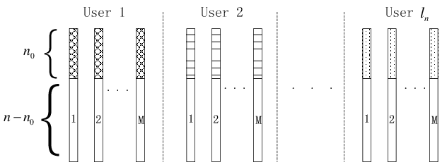
Fig. 4: Codebook structure. Each user maintains MM codewords with each consisting of a message-bearing codeword prepended by a signature.

We first assume unbounded knk_{n} and establish the achievability result. The case of bounded knk_{n} is then straightforward.

We consider a two-stage approach: In the first stage, the set of active users are identified based on their unique signatures. In the second stage, the messages from the active users are decoded. Let θn\theta_{n} and its limit θ\theta be defined as in Theorem 1. We consider the cases of θ=0\theta=0 and θ>0\theta>0 at the same time. Fix ϵ∈(0,min⁡(1,P))\epsilon\in(0,\min(1,P)). Specifically, the following scheme is used:

  • •

    Codebook construction: The codebooks of the ℓn\ell_{n} users are generated independently. Let

    n0={ϵ​n,if ​θ=0(1+ϵ)​θn​n,otherwise .\displaystyle n_{0}=\begin{cases}\epsilon n,&\text{if }\theta=0\\ \left(1+\epsilon\right)\theta_{n}n,&\text{otherwise }.\end{cases} (85)

    For user kk, codeword 𝒔k​(0)=𝟎{\boldsymbol{s}}_{k}(0)=\mathbf{0} represents silence. User kk also generates

    M=⌈exp⁡[(1−ϵ)​B​(n)]⌉\displaystyle M=\lceil\exp\left[(1-\epsilon)B(n)\right]\rceil (86)

    codewords as follows. First, generate MM random sequences of length n−n0n-n_{0}, each according to i.i.d. Gaussian distribution with zero mean and variance P′=P−ϵP^{\prime}=P-\epsilon. Then generate one signature of length n0n_{0} with i.i.d. 𝒩⁡(0,P′)\mathcal{N}(0,P^{\prime}), denoted by 𝑺ka{\boldsymbol{S}}_{k}^{a}, and prepend this signature to every codeword to form MM codewords of length nn. In other words, the ww-th codeword of user kk takes the shape of 𝑺k​(w)=(𝑺ka𝑺kb​(w)){\boldsymbol{S}}_{k}(w)=\left(\begin{smallmatrix}{\boldsymbol{S}}_{k}^{a}\\ {\boldsymbol{S}}_{k}^{b}(w)\end{smallmatrix}\right). The matrix of the concatenated codebooks of all users is illustrated in Fig. 4.

  • •

    Transmission: For user kk to be silent, it is equivalent to transmitting 𝒔k​(0){\boldsymbol{s}}_{k}(0). Otherwise, to send message wk≠0w_{k}\neq 0, user kk transmits 𝑺k​(wk){\boldsymbol{S}}_{k}(w_{k}).

  • •

    Channel: Each user is active independently with probability αn\alpha_{n}. The active users transmit simultaneously. The received signal is 𝒀{\boldsymbol{Y}} given by (5).

  • •

    Two-stage detection and decoding: Upon receiving 𝒀{\boldsymbol{Y}}, the decoder performs the following:

    1) Active user identification: Let 𝒀a{\boldsymbol{Y}}^{a} denote the first n0n_{0} entries of 𝒀{\boldsymbol{Y}}, corresponding to the superimposed signatures of all active users subject to noise. 𝒀a{\boldsymbol{Y}}^{a} is mathematically described by (17). The receiver detects 𝑿a{\boldsymbol{X}}^{a} according to (43). The output of this stage is a set A⊆{1,⋯,ℓn}A\subseteq\{1,\cdots,\ell_{n}\} that contains the detected active users.

    2) Message decoding: Let 𝒀b{\boldsymbol{Y}}^{b} denote the last n−n0n-n_{0} entries of 𝒀{\boldsymbol{Y}}, corresponding to the superimposed message-bearing codewords. The receiver solves the following optimization problem:

    minimize\displaystyle\minimize\quad ‖𝒀b−𝑺¯b​[𝒙1T,⋯,𝒙ℓnT]T‖2\displaystyle\Big\|{\boldsymbol{Y}}^{b}-{\underline{\boldsymbol{S}}}^{b}\left[{\boldsymbol{x}}_{1}^{T},\cdots,{\boldsymbol{x}}_{\ell_{n}}^{T}\right]^{T}\Big\|^{2} (87a)
    subject~to\displaystyle\subjectto\quad 𝒙k∈𝒳M1,k=1,⋯,ℓn\displaystyle{\boldsymbol{x}}_{k}\in\mathcal{X}_{M}^{1},\;k=1,\cdots,\ell_{n} (87b)
    𝒙k=𝟎,∀k∉A\displaystyle{\boldsymbol{x}}_{k}=\mathbf{0},\quad\forall k\notin A (87c)
    𝒙k≠𝟎,∀k∈A.\displaystyle{\boldsymbol{x}}_{k}\neq\mathbf{0},\quad\forall k\in A. (87d)

    Basically the receiver performs the maximum likelihood decoding for the set of users in the purported active user set AA. The position of 1 in each recovered nonzero 𝒙k{\boldsymbol{x}}_{k} indicates the message from user kk.

Theorem 3 (Achievability of the Gaussian many-access channel)

Let θn\theta_{n} be defined as (11) and B⁡(n)B(n) be defined as (12). Suppose limn→∞θn<1\lim_{n\to\infty}\theta_{n}<1. For the MnAC given by (1), for any given constant ϵ∈(0,1)\epsilon\in(0,1), the message length of (1−ϵ)​B​(n)(1-\epsilon)B(n) is asymptotically achievable using the preceding scheme.

The remainder of this section is devoted to the proof of Theorem 3. In Section V-C, we show that the set of active users can be accurately identified in the first stage. In Section V-D, we show that the users’ messages can be accurately decoded in second stage assuming knowledge of the active users. The results are combined in Section V-E to establish the achievability part of Theorem 3.

V-C Optimal User Identification

We shall invoke Theorem 2 (proved in Section IV) to quantify the cost of reliable user identification. To adapt to the notation in this section, we apply Theorem 2 with ℓ\ell and kℓk_{\ell} being replaced by ℓn\ell_{n} and knk_{n}, respectively. With the change of notations, n⁡(ℓ)n(\ell) as defined in Theorem 2 can be written as

n⁡(ℓ)\displaystyle n(\ell) =ℓn​H2​(kn/ℓn)12​log⁡(1+kn​P)\displaystyle=\frac{\ell_{n}H_{2}(k_{n}/\ell_{n})}{\frac{1}{2}\log(1+k_{n}P)} (88)
=θn​n,\displaystyle=\theta_{n}n, (89)

where θn\theta_{n} is given by (11).

According to Theorem 2, choosing the signature length n0=(1+ϵ)​θn​nn_{0}=(1+\epsilon)\theta_{n}n and n0=ϵ​knn_{0}=\epsilon k_{n} yields vanishing error probability in user identification for the case of limn→∞θn​n/kn>0\lim_{n\to\infty}\theta_{n}n/k_{n}>0 and limn→∞θn​n/kn=0\lim_{n\to\infty}\theta_{n}n/k_{n}=0, respectively, where ϵ∈(0,1)\epsilon\in(0,1) is an arbitrary constant. In the following, we make use of this result to prove that choosing n0n_{0} according to (85) guarantees reliable user identification.

First, consider θ=0\theta=0. By (85), the signature length is n0=ϵ​nn_{0}=\epsilon n for some ϵ\epsilon. In the case of limn→∞θn​n/kn>0\lim_{n\to\infty}\theta_{n}n/k_{n}>0, since θn\theta_{n} vanishes, we must have n0≥n(1+ϵ)θnnn_{0}\geq_{n}(1+\epsilon)\theta_{n}n. In the case of limn→∞θn​n/kn=0\lim_{n\to\infty}\theta_{n}n/k_{n}=0, since kn=O⁡(n)k_{n}=O(n), n0=ϵ​nn_{0}=\epsilon n implies n0≥nϵ′knn_{0}\geq_{n}\epsilon^{\prime}k_{n} for some ϵ′>0\epsilon^{\prime}>0. By Theorem 2, the choice of n0n_{0} is sufficient for reliable user identification.

Second, consider θ>0\theta>0. By (85), the signature length is n0=(1+ϵ)​θn​nn_{0}=(1+\epsilon)\theta_{n}n. Since kn=O⁡(n)k_{n}=O(n), we must have limn→∞θn​n/kn>0\lim_{n\to\infty}\theta_{n}n/k_{n}>0. Thus, the signature length n0n_{0} obviously achieves reliable user identification by Theorem 2.

V-D Achieving the MnAC Capacity with Known User Activities

In [1], we studied a Gaussian MnAC where all users are always active and the number of users is sublinear in the blocklength, i.e., kn=o⁡(n)k_{n}=o(n). In that case, random coding and Feinstein’s suboptimal decoding, which achieve the capacity of conventional multiaccess channel, can also achieve the capacity of the Gaussian MnAC. Proving the achievability for faster scaling of the number of active users is much more challenging, mainly because the exponential number of possible error events prevents one from using the simple union bound. Here, we derive the capacity of the MnAC for the case where the number of users may grow as quickly as linearly with the blocklength by lower bounding the error exponent of the error probability due to maximum-likelihood decoding.

Theorem 4 (Capacity of the Gaussian many-access channel without random access)

For the MnAC with knk_{n} always-active users, suppose the number of channel uses is nn and the number of users knk_{n} grows as O⁡(n)O(n), the symmetric capacity is

B1​(n)=n2​kn​log⁡(1+kn​P).\displaystyle B_{1}(n)=\frac{n}{2k_{n}}\log(1+k_{n}P). (90)

In particular, for any ϵ∈(0,1)\epsilon\in(0,1), there exists a sequence of codebooks with message lengths (in nats) B1​(n)​(1−ϵ)B_{1}(n)(1-\epsilon) such that the average error probability is arbitrarily small for sufficiently large nn.

We prove Theorem 4 in the remainder of this subsection. We can model the MnAC with known user activities using (5) with αn=1\alpha_{n}=1, i.e., kn=ℓnk_{n}=\ell_{n}. Upon receiving the length-nn vector 𝒚{\boldsymbol{y}}, we estimate 𝒙=[𝒙1T,⋯,𝒙knT]T{\boldsymbol{x}}=\left[{\boldsymbol{x}}^{T}_{1},\cdots,{\boldsymbol{x}}^{T}_{k_{n}}\right]^{T} using the maximum likelihood decoding:

minimize\displaystyle\minimize\quad ‖𝒚−𝒔¯​𝒙‖2\displaystyle\|{\boldsymbol{y}}-{\underline{\boldsymbol{s}}}{\boldsymbol{x}}\|^{2} (91a)
subject~to\displaystyle\subjectto\quad 𝒙k=𝒆m​for some ​m=1,⋯,M.\displaystyle{\boldsymbol{x}}_{k}={\boldsymbol{e}}_{m}\;\;\text{for some }m=1,\cdots,M. (91b)

Define ℱj\mathcal{F}_{j} as the event that user jj’s codeword violates the power constraint (2), j=1,⋯,knj=1,\cdots,k_{n}. Define ℰk\mathcal{E}_{k} as the error event that kk users are received in error. Suppose 𝖯​{ℰk|A∗}\mathsf{P}\{\mathcal{E}_{k}|A^{\ast}\} is the probability of ℰk\mathcal{E}_{k} given that the true signal is 𝒙∗{\boldsymbol{x}}^{\ast} with support A∗A^{\ast}. By symmetry of the codebook construction, the average error probability can be upper bounded as

𝖯e(n)\displaystyle\mathsf{P}_{e}^{(n)} ≤𝖯{(∪k=1knℰk)∪(∪j=1knℱj)}\displaystyle\leq\mathsf{P}\left\{\left(\cup_{k=1}^{k_{n}}\mathcal{E}_{k}\right)\cup\left(\cup_{j=1}^{k_{n}}\mathcal{F}_{j}\right)\right\} (92)
≤1Mkn​∑A∗∑k=1kn𝖯⁡{ℰk|A∗}+∑j=1kn𝖯⁡{ℱj}.\displaystyle\leq\frac{1}{M^{k_{n}}}\sum_{A^{\ast}}\sum_{k=1}^{k_{n}}\mathsf{P}\{\mathcal{E}_{k}|A^{\ast}\}+\sum_{j=1}^{k_{n}}\mathsf{P}\left\{\mathcal{F}_{j}\right\}. (93)

Let AA be the support of the estimated 𝒙{\boldsymbol{x}} according to the maximum likelihood decoding. Define A1A_{1} and A2A_{2} in the same manner as that in Section V-C, i.e., A1=A∗\AA_{1}=A^{\ast}\backslash A and A2=A\A∗A_{2}=A\backslash A^{\ast}. In this case, |A|=|A∗|=kn|A|=|A^{\ast}|=k_{n} and |A2|=|A1|=k|A_{2}|=|A_{1}|=k. Further denote γ=k/kn\gamma=k/k_{n} as the fraction of users subjected to errors. Then we write 𝖯​{ℰk|A∗}\mathsf{P}\{\mathcal{E}_{k}|A^{\ast}\} and 𝖯​{ℰγ|A∗}\mathsf{P}\{\mathcal{E}_{\gamma}|A^{\ast}\} interchangeably. In the following analysis, we consider a fixed A∗A^{\ast} and drop the conditioning on A∗A^{\ast} for notational convenience. Following similar arguments leading to (74), letting λ=11+ρ\lambda=\frac{1}{1+\rho} and considering (knγ​kn)\binom{k_{n}}{\gamma k_{n}} possible sets of A1A_{1} and Mγ​knM^{\gamma k_{n}} possible sets of A2A_{2}, we have

𝖯​{ℰγ}\displaystyle\mathsf{P}\{\mathcal{E}_{\gamma}\} ≤(knγ​kn)Mγ​kn​ρ(∫ℝ𝖤{pY|𝑺A1ρ+1(y|𝑺A∗)×\displaystyle\leq\binom{k_{n}}{\gamma k_{n}}M^{\gamma k_{n}\rho}\left(\int_{\mathbb{R}}\mathsf{E}\left\{p^{\frac{1}{\rho+1}}_{Y|{\boldsymbol{S}}_{A}}(y|{\boldsymbol{S}}_{A^{\ast}})\times\right.\right.
(𝖤{pY|𝑺A1ρ+1(y|𝑺A)|𝑺A∗})ρ}dy)n\displaystyle\qquad\left.\left.\left(\mathsf{E}\left\{p^{\frac{1}{\rho+1}}_{Y|{\boldsymbol{S}}_{A}}(y|{\boldsymbol{S}}_{A})\Big|{\boldsymbol{S}}_{A^{\ast}}\right\}\right)^{\rho}\right\}dy\right)^{n} (94)
=(knγ​kn)Mγ​kn​ρ×\displaystyle=\binom{k_{n}}{\gamma k_{n}}M^{\gamma k_{n}\rho}\times
(∫ℝ𝖤{𝖤{pY|𝑺A1ρ+1(y|𝑺A∗)|𝑺A∗∩A}×\displaystyle\quad\left(\int_{\mathbb{R}}\mathsf{E}\left\{\mathsf{E}\left\{p^{\frac{1}{\rho+1}}_{Y|{\boldsymbol{S}}_{A}}(y|{\boldsymbol{S}}_{A^{\ast}})\Big|{\boldsymbol{S}}_{A^{\ast}\cap A}\right\}\times\right.\right.
(𝖤{pY|𝑺A1ρ+1(y|𝑺A)|𝑺A∗})ρ}dy)n.\displaystyle\quad\left.\left.\left(\mathsf{E}\left\{p^{\frac{1}{\rho+1}}_{Y|{\boldsymbol{S}}_{A}}(y|{\boldsymbol{S}}_{A})\Big|{\boldsymbol{S}}_{A^{\ast}}\right\}\right)^{\rho}\right\}dy\right)^{n}. (95)

By symmetry,

𝖤⁡{pY|𝑺A1ρ+1​(y|𝑺A)|𝑺A∗}=𝖤⁡{pY|𝑺A1ρ+1​(y|𝑺A∗)|𝑺A∗∩A},\displaystyle\mathsf{E}\left\{p^{\frac{1}{\rho+1}}_{Y|{\boldsymbol{S}}_{A}}(y|{\boldsymbol{S}}_{A})\Big|{\boldsymbol{S}}_{A^{\ast}}\right\}=\mathsf{E}\left\{p^{\frac{1}{\rho+1}}_{Y|{\boldsymbol{S}}_{A}}(y|{\boldsymbol{S}}_{A^{\ast}})\Big|{\boldsymbol{S}}_{A^{\ast}\cap A}\right\}, (96)

which results in

𝖯​{ℰγ}\displaystyle\mathsf{P}\{\mathcal{E}_{\gamma}\} ≤(knγ​kn)​Mγ​kn​ρ​exp⁡(−n​E0​(γ,ρ)),\displaystyle\leq\binom{k_{n}}{\gamma k_{n}}M^{\gamma k_{n}\rho}\exp(-nE_{0}(\gamma,\rho)), (97)

where E0​(γ,ρ)E_{0}(\gamma,\rho) is defined by

E0​(γ,ρ)=\displaystyle E_{0}(\gamma,\rho)=
−log⁡[∫ℝ𝖤⁡{[𝖤⁡{(pY|𝑺A​(y|𝑺A))1ρ+1|𝑺A∗}]1+ρ}​𝑑y].\displaystyle-\log\left[\int_{\mathbb{R}}\mathsf{E}\left\{\left[\mathsf{E}\left\{\left(p_{Y|{\boldsymbol{S}}_{A}}(y|{\boldsymbol{S}}_{A})\right)^{\frac{1}{\rho+1}}\Big|{\boldsymbol{S}}_{A^{\ast}}\right\}\right]^{1+\rho}\right\}dy\right]. (98)

By the inequality

(knγ​kn)≤exp⁡(kn​H2​(γ)),\displaystyle\binom{k_{n}}{\gamma k_{n}}\leq\exp(k_{n}H_{2}(\gamma)), (99)

we can further upper bound 𝖯​{ℰγ}\mathsf{P}\{\mathcal{E}_{\gamma}\} as

𝖯⁡{ℰγ}≤exp⁡[−n​f​(γ,ρ)],\displaystyle\mathsf{P}\{\mathcal{E}_{\gamma}\}\leq\exp\left[-nf(\gamma,\rho)\right], (100)

where

f⁡(γ,ρ)=E0​(γ,ρ)−γ​ρ​knn​v​(n)−knn​H2​(γ),\displaystyle f(\gamma,\rho)=E_{0}(\gamma,\rho)-\gamma\rho\frac{k_{n}}{n}v(n)-\frac{k_{n}}{n}H_{2}(\gamma), (101)

and v⁡(n)=log⁡Mv(n)=\log M. Intuitively, E0​(γ,ρ)E_{0}(\gamma,\rho) in (100) is an achievable error exponent for the error probability caused by a particular AA being detected in favor of A∗A^{\ast} and the terms kn​H2​(γ)+γ​ρ​kn​v​(n)k_{n}H_{2}(\gamma)+\gamma\rho k_{n}v(n) correspond to the cardinality of all possible AA leading to the error event ℰγ\mathcal{E}_{\gamma}.

By (75), it is straightforward to show that

E0​(γ,ρ)\displaystyle E_{0}(\gamma,\rho) =−log⁡mλ,ρ​(w1,w2)|w1=w2=γ​kn,λ=11+ρ.\displaystyle=-\log m_{\lambda,\rho}(w_{1},w_{2})|_{w_{1}=w_{2}=\gamma k_{n},\lambda=\frac{1}{1+\rho}}. (102)

By particularizing (77) with w1=w2=γ​knw_{1}=w_{2}=\gamma k_{n} and λ=11+ρ\lambda=\frac{1}{1+\rho}, we can derive E0​(γ,ρ)E_{0}(\gamma,\rho) explicitly as

E0​(γ,ρ)\displaystyle E_{0}(\gamma,\rho) =ρ2​log⁡(1+γ​kn​P′ρ+1).\displaystyle=\frac{\rho}{2}\log\left(1+\frac{\gamma k_{n}P^{\prime}}{\rho+1}\right). (103)

The achievable error exponent for P⁡(ℰγ)P(\mathcal{E}_{\gamma}) is determined by the minimum error exponent over the range of γ\gamma, i.e.,

Er=min1kn≤γ≤1⁡max0≤ρ≤1⁡f⁡(γ,ρ).\displaystyle E_{r}=\min_{\frac{1}{k_{n}}\leq\gamma\leq 1}\max_{0\leq\rho\leq 1}f(\gamma,\rho). (104)
Lemma 4

Let MM be such that the message length v⁡(n)=log⁡Mv(n)=\log M is given by

v⁡(n)=(1−ϵ)​n2​kn​log⁡(1+kn​P′).\displaystyle v(n)=(1-\epsilon)\frac{n}{2k_{n}}\log(1+k_{n}P^{\prime}). (105)

Suppose kn=O⁡(n)k_{n}=O(n), there exists n∗n^{\ast} and c0>0c_{0}>0 such that for every n≥n∗n\geq n^{\ast},

𝖯⁡{ℰk|A∗}≤e−c0​n\displaystyle\mathsf{P}\{\mathcal{E}_{k}|A^{\ast}\}\leq e^{-c_{0}n} (106)

holds uniformly for all 1≤k≤kn1\leq k\leq k_{n} and for all |A∗||A^{\ast}|.

Proof:

See Appendix E. ∎

Due to Lemma 4, for large enough nn,

∑k=1kn𝖯⁡{ℰk|A∗}≤kn​e−c0​n\displaystyle\sum_{k=1}^{k_{n}}\mathsf{P}\{\mathcal{E}_{k}|A^{\ast}\}\leq k_{n}e^{-c_{0}n} (107)

which vanishes as nn increases. Moreover, following the same argument as (48), the second term of the RHS of (93) vanishes and hence 𝖯e(n)\mathsf{P}_{e}^{(n)} given by (93) can be proved to vanish. As a result, Theorem 4 is established.

V-E Achieving the Capacity of MnAC with Random Access

In this subsection, we combine the results of Section V-C and Section V-D to prove the achievability result for Case 1 and Case 2 in Theorem 3. We first prove the case of unbounded knk_{n}, and the case of bounded knk_{n} follows naturally. Let θ\theta denote the limit of θn\theta_{n}.

Case 1) unbounded ℓn\ell_{n} and unbounded knk_{n}.

We further divide this case into two sub-cases.

Sub-case a) 0<θ<10<\theta<1: We shall show that the message length (1−ϵ)​B​(n)(1-\epsilon)B(n) is asymptotically achievable for every ϵ∈(0,1)\epsilon\in(0,1).

The detection errors are caused by activity identification error or message decoding error. It has been shown by (53) that with high probability the number of active users is no more than (1+δn)​kn(1+\delta_{n})k_{n}. As a result, Theorem 2 and Theorem 4 conclude that the message length

(1−ϵ′)​(n−n0)2​(1+δn)​kn​log⁡(1+(1+δn)​kn​P),\displaystyle\frac{(1-\epsilon^{\prime})(n-n_{0})}{2(1+\delta_{n})k_{n}}\log\left(1+(1+\delta_{n})k_{n}P\right), (108)

where n0=(1+ϵ′)​θn​nn_{0}=(1+\epsilon^{\prime})\theta_{n}n, is asymptotically achievable for any ϵ′>0\epsilon^{\prime}>0, when the number of active user is (1+δn)​kn(1+\delta_{n})k_{n}. Therefore, the message length (108) is aymptotically achievable for any fewer number of active users.

In order to prove the achievability, it suffices to show that there exists ϵ′\epsilon^{\prime} such that the message length given by (108) is asymptotically greater than

(1−ϵ)​B​(n)=(1−ϵ)​(1−θn)​n2​kn​log⁡(1+kn​P).\displaystyle(1-\epsilon)B(n)=\frac{(1-\epsilon)(1-\theta_{n})n}{2k_{n}}\log\left(1+k_{n}P\right). (109)

The intuition of proof is that for sufficiently large nn, (1+δn)​kn(1+\delta_{n})k_{n} is approximately knk_{n}, and we can always find a small enough ϵ′\epsilon^{\prime} such that (1−ϵ′)​(n−n0)(1-\epsilon^{\prime})(n-n_{0}) is greater than (1−ϵ)​(1−θn)​n(1-\epsilon)(1-\theta_{n})n.

We choose some small enough ϵ′>0\epsilon^{\prime}>0 such that

(1−ϵ′)2−ϵ′​(1−ϵ′)2​1+θ1−θ>1−ϵ.\displaystyle(1-\epsilon^{\prime})^{2}-\epsilon^{\prime}(1-\epsilon^{\prime})^{2}\frac{1+\theta}{1-\theta}>1-\epsilon. (110)

This is feasible because the left-hand side of (110) is equal to 1 if ϵ′=0\epsilon^{\prime}=0.

Since log⁡(1+(1+δn)​kn​P)/log⁡(1+kn​P)→1\log\left(1+(1+\delta_{n})k_{n}P\right)/\log(1+k_{n}P)\to 1 and δn→0\delta_{n}\to 0 as nn increases, we have

log⁡(1+(1+δn)​kn​P)(1+δn)≥n(1−ϵ′)log(1+knP).\displaystyle\frac{\log\left(1+(1+\delta_{n})k_{n}P\right)}{(1+\delta_{n})}\geq_{n}(1-\epsilon^{\prime})\log(1+k_{n}P). (111)

The difference between (108) and (1−ϵ)​B​(n)(1-\epsilon)B(n) is equal to

(1−ϵ′)​(n−n0)2​(1+δn)​kn​log⁡(1+(1+δn)​kn​P)−(1−ϵ)​B​(n)\displaystyle\frac{(1-\epsilon^{\prime})(n-n_{0})}{2(1+\delta_{n})k_{n}}\log\left(1+(1+\delta_{n})k_{n}P\right)-(1-\epsilon)B(n)
≥n[(1−ϵ′)2​(1−n0/n)1−θn−(1−ϵ)]B(n)\displaystyle\geq_{n}\left[\frac{(1-\epsilon^{\prime})^{2}(1-n_{0}/n)}{1-\theta_{n}}-(1-\epsilon)\right]B(n) (112)
=[(1−ϵ′)2−ϵ′​(1−ϵ′)2​θn1−θn−(1−ϵ)]​B​(n)\displaystyle=\left[(1-\epsilon^{\prime})^{2}-\epsilon^{\prime}(1-\epsilon^{\prime})^{2}\frac{\theta_{n}}{1-\theta_{n}}-(1-\epsilon)\right]B(n) (113)
≥n[(1−ϵ′)2−ϵ′(1−ϵ′)21+θ1−θ−(1−ϵ)]B(n)\displaystyle\geq_{n}\left[(1-\epsilon^{\prime})^{2}-\epsilon^{\prime}(1-\epsilon^{\prime})^{2}\frac{1+\theta}{1-\theta}-(1-\epsilon)\right]B(n) (114)

where (114) is due to θn≤n(1+θ)/2\theta_{n}\leq_{n}(1+\theta)/2. By (110), the RHS of (114) is greater than zero. It means that for large enough nn, the achievabile message length (108) is greater than (1−ϵ)​B​(n)(1-\epsilon)B(n), which establishes the achievability.

Sub-case b) θ=0\theta=0: The proof for the case of vanishing θn\theta_{n} is analogous. We shall show that message length (1−ϵ)​B1​(n)(1-\epsilon)B_{1}(n) is asymptotically achievable for all ϵ∈(0,1)\epsilon\in(0,1).

The number of active users is no more than (1+δn)​kn(1+\delta_{n})k_{n} with high probability. As a result, Theorem 2 and Theorem 4 conclude that the message length

(1−ϵ′)​(n−n0)2​(1+δn)​kn​log⁡(1+(1+δn)​kn​P),\displaystyle\frac{(1-\epsilon^{\prime})(n-n_{0})}{2(1+\delta_{n})k_{n}}\log\left(1+(1+\delta_{n})k_{n}P\right), (115)

where n0=ϵ′​nn_{0}=\epsilon^{\prime}n, is asymptotically achievable for all ϵ′>0\epsilon^{\prime}>0.

In order to prove Theorem 3, it suffices to show that there exists ϵ′\epsilon^{\prime} such that the message length given by (115) is asymptotically greater than

(1−ϵ)​B1​(n)=(1−ϵ)​n2​kn​log⁡(1+kn​P).\displaystyle(1-\epsilon)B_{1}(n)=(1-\epsilon)\frac{n}{2k_{n}}\log\left(1+k_{n}P\right). (116)

Choose some small enough ϵ′>0\epsilon^{\prime}>0 such that

(1−ϵ′)3>(1−ϵ).\displaystyle(1-\epsilon^{\prime})^{3}>(1-\epsilon). (117)

The difference between (115) and (1−ϵ)​B1​(n)(1-\epsilon)B_{1}(n) is equal to

(1−ϵ′)​(n−n0)2​(1+δn)​kn​log⁡(1+(1+δn)​kn​P)−(1−ϵ)​B1​(n)\displaystyle\frac{(1-\epsilon^{\prime})(n-n_{0})}{2(1+\delta_{n})k_{n}}\log\left(1+(1+\delta_{n})k_{n}P\right)-(1-\epsilon)B_{1}(n)
≥n[(1−ϵ′)2(1−n0/n)−(1−ϵ)]B1(n)\displaystyle\geq_{n}\left[(1-\epsilon^{\prime})^{2}(1-n_{0}/n)-(1-\epsilon)\right]B_{1}(n) (118)
=[(1−ϵ′)3−(1−ϵ)]​B​(n),\displaystyle=\left[(1-\epsilon^{\prime})^{3}-(1-\epsilon)\right]B(n), (119)

where (118) is due to (111). By the choice of ϵ′\epsilon^{\prime} given by (117), (119) is greater than zero. It concludes that for large enough nn, the achievable message length (115) is greater than (1−ϵ)​B1​(n)(1-\epsilon)B_{1}(n), which establishes the achievability.

Case 2) unbounded ℓn\ell_{n} and bounded knk_{n}.

In this case, there is nonvanishing probability that the number of active users is equal to any finite number. The number of active users is no longer fewer than (1+δn)​kn(1+\delta_{n})k_{n} with high probability. Let sns_{n} be any increasing sequence. There is high probability that the number of users is fewer than (1+δn)​sn(1+\delta_{n})s_{n}. As a result, by treating sns_{n} as the unbounded knk_{n} as in Case 1, we can apply the established achievable results for Case 1. The achievability result for Case 2 is summarized in the following theorem.

Theorem 5

Suppose ℓn\ell_{n} is unbounded and knk_{n} is bounded. Let sns_{n} be any increasing sequence satisfying sn=O⁡(n)s_{n}=O(n), ℓn​e−δ​sn→0\ell_{n}e^{-\delta s_{n}}\to 0 for every δ>0\delta>0 and

limn→∞2​ℓn​H2​(sn/ℓn)n​log⁡(1+sn​P)<1.\displaystyle\lim_{n\to\infty}\frac{2\ell_{n}H_{2}(s_{n}/\ell_{n})}{n\log(1+s_{n}P)}<1. (120)

Then every message length given by

(1−ϵ)​(n2​sn​log⁡(1+sn​P)−H2​(snℓn))\displaystyle(1-\epsilon)\left(\frac{n}{2s_{n}}\log(1+s_{n}P)-H_{2}\left(\frac{s_{n}}{\ell_{n}}\right)\right) (121)

is asymptotically achievable.

Proof:

See Appendix F. ∎

Recall that according to Theorem 1, any message length growing linearly in nn is not achievabile under the conditions of Theorem 5. Theorem 5 states that the message length given by (121), which grows sublinearly in nn, is achievable.

VI Successive Decoding for MnAC

In conventional multiaccess channels, the sum capacity can be achieved by successive decoding. A natural question is: Can the sum capacity of the MnAC be achieved using successive decoding? We consider the system model where all users have the same power constraints, assuming no random activity and the number of users being kn=a​nk_{n}=an for some a>0a>0. We provide a negative answer for the case where Gaussian random codes are used and successive decoding is applied. Throughout the discussion in this section, we do not insist on symmetric message lengths.

Suppose Gaussian random codes are used, i.e., each user generates its codewords as i.i.d. Gaussian random variables with zero mean and variance PP. Thus the codewords of other users look like Gaussian noise to any given user. The first user to be decoded has the largest interference from all the other kn−1k_{n}-1 users and its signal-to-interference-plus-noise ratio (SINR) is Q=P/(1+(kn−1)​P)Q=P/(1+(k_{n}-1)P). Suppose the first user transmits with message length

v⁡(n)=(1−ϵ)​n​C,\displaystyle v(n)=(1-\epsilon)nC, (122)

where C=12​log⁡(1+Q)C=\frac{1}{2}\log(1+Q). We will show that the error probability is strictly bounded from zero. The intuition is that the error probability usually decays at the rate of exp⁡(−δ​n​C)\exp(-\delta nC), where δ\delta is some positive constant dependent on ϵ\epsilon. In the MnAC setting, if the interference due to many users is so large that n​CnC converges to a finite constant, the error exponent is not large enough to drive the error probability to zero as the blocklengh increases.

Lemma 5

Suppose Gaussian random codes are used and successive decoding is applied. There exist universal constants d1>0d_{1}>0 and d2>0d_{2}>0, such that the error probability of the first user is lower bounded as

𝖯e(n)≥𝖰⁡(x)​e−d1​T​x3S3/2​(1−d2​T​xS3/2)−e−(λ−1)​(n−1)​ϵ​C,\displaystyle\mathsf{P}_{e}^{(n)}\geq\mathsf{Q}(x)e^{-\frac{d_{1}Tx^{3}}{S^{3/2}}}\left(1-\frac{d_{2}Tx}{S^{3/2}}\right)-e^{-(\lambda-1)(n-1)\epsilon C}, (123)

where 𝖰⁡(x)=12​π​∫x∞exp⁡(−u22)​𝑑u\mathsf{Q}(x)=\frac{1}{\sqrt{2\pi}}\int_{x}^{\infty}\exp(-\frac{u^{2}}{2})du, S=2​n​Q​(2+Q)S=2nQ(2+Q),

x=2​(λ​ϵ​n+1−λ​ϵ)​C​(1+Q)​S−12,\displaystyle x=2(\lambda\epsilon n+1-\lambda\epsilon)C(1+Q)S^{-\frac{1}{2}}, (124)

and

T=n​𝖤​{(−Q⁡(1−Z2)−2​Q​Z)3}\displaystyle T=n\mathsf{E}\left\{(-Q(1-Z^{2})-2\sqrt{Q}Z)^{3}\right\} (125)

where ZZ is a standard Gaussian random variable.

Proof:

See Appendix G. ∎

Let kn=a​nk_{n}=an for some constant a>0a>0. Then, as n→∞n\to\infty, we have n​Q→1/anQ\to{1}/{a}, S→4/aS\to{4}/{a}, T→0T\to 0, n​C→1/(2​a)nC\to{1}/{(2a)}, and x→ϵ​λ/(2​a)x\to{\epsilon\lambda}/{(2\sqrt{a})}. Therefore,

limn→∞𝖯e(n)≥𝖰⁡(ϵ​λ2​a)−e−(λ−1)​ϵ2​a.\displaystyle\lim_{n\to\infty}\mathsf{P}_{e}^{(n)}\geq\mathsf{Q}\left(\frac{\epsilon\lambda}{2\sqrt{a}}\right)-e^{-\frac{(\lambda-1)\epsilon}{2a}}. (126)
Refer to caption
Fig. 5: Lower bound of error probability given by (126) for successive decoding with ϵ=10−3\epsilon=10^{-3}.

Using the lower bound 𝖰(x)≥12​π(1x−1x3)e−x2/2\mathsf{Q}(x)\geq\frac{1}{\sqrt{2\pi}}\left(\frac{1}{x}-\frac{1}{x^{3}}\right)e^{-x^{2}/2}, it can be seen that when the exponential term is dominating, there exists some small enough λ​ϵ\lambda\epsilon such that the first term in (126) is greater than the second term. In this case, the error probability is strictly bounded away from zero. Fig. 5 plots the numerical results of the RHS of (126) for different values of aa and λ\lambda. It can be seen that for the different values of aa, there exists some λ\lambda that makes the lower bound of error probability (126) strictly greater than zero.

VII MnAC with Heterogeneous User Groups

In this section, we will generalize the characterization of capacity region to the case where groups of users have heterogeneous channel gains and activity patterns. Suppose ℓn\ell_{n} users can be divided into a finite number of JJ groups, where group jj consists of β(j)​ℓn\beta^{(j)}\ell_{n} users with ∑j=1Jβ(j)=1\sum_{j=1}^{J}\beta^{(j)}=1. Further assume every user in group jj has the same power constraint P(j)P^{(j)}. Each user in group jj transmits with probability αn(j)\alpha_{n}^{(j)}. We refer to such MnAC with heterogeneous channel gains and activity patterns as the configuration ({αn(j)},{β(j)},{P(j)},ℓn)\left(\{\alpha^{(j)}_{n}\},\{\beta^{(j)}\},\{P^{(j)}\},\ell_{n}\right). The error probability is defined as the probability that the receiver incorrectly detects the message of any user in the system. The problem is what is the maximum achievable message length for users in each group such that the average error probability vanishes.

Definition 5 (Asymptotically achievable message length tuple)

Consider a MnAC of configuration ({αn(j)},{β(j)},{P(j)},ℓn)\left(\{\alpha^{(j)}_{n}\},\{\beta^{(j)}\},\{P^{(j)}\},\ell_{n}\right). A sequence of (⌈exp⁡(v(1)​(n))⌉𝐶𝐿𝑂𝑆𝐸\big(\lceil\exp(v^{(1)}(n))\rceil, ⋯\cdots, 𝑂𝑃𝐸𝑁⌈exp⁡(v(J)​(n))⌉,n)\lceil\exp(v^{(J)}(n))\rceil,n\big) code for this configuration consists of a (⌈exp⁡(v(j)​(n))⌉,n)\left(\lceil\exp(v^{(j)}(n))\rceil,n\right) symmetry code for every user in group jj according to Definition 1, j=1,⋯,Jj=1,\cdots,J. We say a message length tuple (v(1)​(n),⋯,v(J)​(n))\left(v^{(1)}(n),\cdots,v^{(J)}(n)\right) is asymptotically achievable if there exists a sequence of (⌈exp⁡(v(1)​(n))⌉,⋯,⌈exp⁡(v(J)​(n))⌉,n)\left(\lceil\exp(v^{(1)}(n))\rceil,\cdots,\lceil\exp(v^{(J)}(n))\rceil,n\right) codes such that the average error probability vanishes as n→∞n\to\infty.

Definition 6 (Capacity region of the many-access channel)

Consider a MnAC of configuration ({αn(j)},{β(j)},{P(j)},ℓn)\left(\{\alpha^{(j)}_{n}\},\{\beta^{(j)}\},\{P^{(j)}\},\ell_{n}\right). The capacity region is the set of asymptotically achievable message length tuples. In particular, for every (B(1)​(n),⋯,B(J)​(n))\left(B^{(1)}(n),\cdots,B^{(J)}(n)\right) in the capacity region, if the users transmit with message length tuple ((1−ϵ)​B(1)​(n),⋯,(1−ϵ)​B(J)​(n))\left((1-\epsilon)B^{(1)}(n),\cdots,(1-\epsilon)B^{(J)}(n)\right), the average error probability vanishes as n→∞n\to\infty. If users transmit according to a message-length tuple outside the capacity region, then the communication cannot be reliable.

Theorem 6

Consider a MnAC of configuration ({αn(j)},{β(j)},{P(j)},ℓn)\left(\{\alpha^{(j)}_{n}\},\{\beta^{(j)}\},\{P^{(j)}\},\ell_{n}\right). Suppose ℓn→∞\ell_{n}\to\infty and for every j∈{1,…,J}j\in\{1,\dots,J\}, αn(j)→α(j)∈[0,1]\alpha_{n}^{(j)}\to\alpha^{(j)}\in[0,1]. Let the average number of active users in group jj be kn(j)=αn(j)​β(j)​ℓn=O⁡(n)k_{n}^{(j)}=\alpha_{n}^{(j)}\beta^{(j)}\ell_{n}=O(n), such that ℓn​e−δ​kn(j)→0\ell_{n}e^{-\delta k_{n}^{(j)}}\to 0 for all δ>0\delta>0 and j=1,⋯,Jj=1,\cdots,J. Let θn(j)\theta_{n}^{(j)} be defined as

θn(j)=2​β(j)​ℓn​H2​(αn(j))n​log⁡kn(j)\displaystyle\theta_{n}^{(j)}=\frac{2\beta^{(j)}\ell_{n}H_{2}\left(\alpha_{n}^{(j)}\right)}{n\log k_{n}^{(j)}} (127)

and let θ(j)\theta^{(j)} denote its limit. Suppose log⁡kn(j1)/log⁡kn(j2)→1\log k_{n}^{(j_{1})}/\log k_{n}^{(j_{2})}\to 1 for any j1,j2∈{1,⋯,J}j_{1},j_{2}\in\{1,\cdots,J\}. If ∑j=1Jθ(j)<1\sum_{j=1}^{J}\theta^{(j)}<1, then the message length capacity region is characterized as

∑j=1Jkn(j)​B(j)​(n)≤n2​log⁡(∑j=1Jkn(j))−∑j=1Jβ(j)​ℓn​H2​(αn(j)).\displaystyle\sum_{j=1}^{J}k_{n}^{(j)}B^{(j)}(n)\leq\frac{n}{2}\log\left(\sum_{j=1}^{J}k_{n}^{(j)}\right)-\sum_{j=1}^{J}\beta^{(j)}\ell_{n}H_{2}\left(\alpha_{n}^{(j)}\right). (128)

If ∑j=1Jθ(j)>1\sum_{j=1}^{J}\theta^{(j)}>1, then some user cannot transmit a single bit reliably.

As far as the asymptotic message lengths are concerned, the impact of the transmit power is inconsequential. Also, the only limitation on the message is their weighted average. This is in contrast to the classical multiaccess channel, where the sum rate of each subset of users is subject to a separate upper bound in general.

VII-A Converse

The proof of converse follows similarly as in Section III. We only sketch the proof here. Consider the system model described by (5). Suppose the message length transmitted by each user in group jj is v(j)​(n)v^{(j)}(n), j=1,⋯,Jj=1,\cdots,J. Let 𝑿~j\tilde{{\boldsymbol{X}}}_{j} denote a vector, which stacks the vectors 𝑿k{\boldsymbol{X}}_{k}, for all kk belonging to group jj. Since there are a total of β(j)​ℓn\beta^{(j)}\ell_{n} users in group jj and the distributions of 𝑿k{\boldsymbol{X}}_{k} are the same for all kk in the same group jj, we have

H⁡(𝑿~j)\displaystyle H\left(\tilde{{\boldsymbol{X}}}_{j}\right) =β(j)​ℓn​H​(𝑿k)\displaystyle=\beta^{(j)}\ell_{n}H({\boldsymbol{X}}_{k}) (129)
=β(j)​ℓn​(H2​(αn(j))+αn(j)​v(j)​(n)).\displaystyle=\beta^{(j)}\ell_{n}\left(H_{2}\left(\alpha_{n}^{(j)}\right)+\alpha_{n}^{(j)}v^{(j)}(n)\right). (130)

Let GG denote an arbitrary subset of {1,⋯,J}\{1,\cdots,J\} and let G¯\overline{G} denote {1,…,J}∖G\{1,\dots,J\}\setminus G. Further denote 𝑿~G\tilde{{\boldsymbol{X}}}_{G} as the vector consisting of {𝑿~j:j∈G}\{\tilde{{\boldsymbol{X}}}_{j}:j\in G\}. Thus,

H⁡(𝑿~G)\displaystyle H\left(\tilde{{\boldsymbol{X}}}_{G}\right) =∑j∈GH⁡(𝑿~j).\displaystyle=\sum_{j\in G}H\left(\tilde{{\boldsymbol{X}}}_{j}\right). (131)

Applying the chain rule, we have

H\displaystyle H (𝑿~G)=I⁡(𝑿~G,𝒀)+H⁡(𝑿~G|𝒀)\displaystyle\left(\tilde{{\boldsymbol{X}}}_{G}\right)=I\left(\tilde{{\boldsymbol{X}}}_{G};{\boldsymbol{Y}}\right)+H\left(\tilde{{\boldsymbol{X}}}_{G}|{\boldsymbol{Y}}\right) (132)
=H⁡(𝑿~G|𝑿~G¯)−H⁡(𝑿~G|𝒀)+H⁡(𝑿~G|𝒀)\displaystyle=H\left(\tilde{{\boldsymbol{X}}}_{G}|\tilde{{\boldsymbol{X}}}_{\overline{G}}\right)-H\left(\tilde{{\boldsymbol{X}}}_{G}|{\boldsymbol{Y}}\right)+H\left(\tilde{{\boldsymbol{X}}}_{G}|{\boldsymbol{Y}}\right) (133)
≤I⁡(𝑿~G;𝒀|𝑿~G¯)+H⁡(𝑿~G|𝒀).\displaystyle\leq I\left(\tilde{{\boldsymbol{X}}}_{G};{\boldsymbol{Y}}|\tilde{{\boldsymbol{X}}}_{\overline{G}}\right)+H\left(\tilde{{\boldsymbol{X}}}_{G}|{\boldsymbol{Y}}\right). (134)

Following the argument in Lemma 1, we have

I⁡(𝑿~G;𝒀|𝑿~G¯)≤n2​log⁡(1+∑j∈Gkn(j)​P(j)).\displaystyle I\left(\tilde{{\boldsymbol{X}}}_{G};{\boldsymbol{Y}}|\tilde{{\boldsymbol{X}}}_{\overline{G}}\right)\leq\frac{n}{2}\log\left(1+\sum_{j\in G}k_{n}^{(j)}P^{(j)}\right). (135)

In order to achieve vanishing error probability, following the argument in Lemma 2, we have

H⁡(𝑿~G|𝒀)=o⁡(∑j∈Gkn(j)​v(j)​(n)+β(j)​ℓn​H2​(αn(j))).\displaystyle H\left(\tilde{{\boldsymbol{X}}}_{G}|{\boldsymbol{Y}}\right)=o\left(\sum_{j\in G}k_{n}^{(j)}v^{(j)}(n)+\beta^{(j)}\ell_{n}H_{2}\left(\alpha^{(j)}_{n}\right)\right). (136)

Combining (130), (131), (134), (135), and (136), we have

(1−ϵ)∑j∈G[kn(j)​v(j)​(n)+β(j)​ℓn​H2​(αn(j))]≤n2​log⁡(1+∑j∈Gkn(j)​P(j)),\displaystyle\begin{split}(1-\epsilon)&\sum_{j\in G}\left[k_{n}^{(j)}v^{(j)}(n)+\beta^{(j)}\ell_{n}H_{2}\left(\alpha_{n}^{(j)}\right)\right]\\ &\leq\frac{n}{2}\log\left(1+\sum_{j\in G}k_{n}^{(j)}P^{(j)}\right),\end{split} (137)

for all ϵ>0\epsilon>0 and large enough nn.

Since the power in each group is bounded, we have

limn→∞log⁡(1+∑j∈Gkn(j)​P(j))log∑j∈Gkn(j)=1.\displaystyle\lim_{n\to\infty}\frac{\log\left(1+\sum_{j\in G}k_{n}^{(j)}P^{(j)}\right)}{\log\sum_{j\in G}k_{n}^{(j)}}=1. (138)

Thus, (137) implies that for every ϵ>0\epsilon>0,

∑j∈Gkn(j)​v(j)​(n)≤(1+ϵ)​n2​log⁡(∑j∈Gkn(j))−∑j∈Gβ(j)​ℓn​H2​(αn(j)).\displaystyle\begin{split}&\sum_{j\in G}k_{n}^{(j)}v^{(j)}(n)\leq\\ &\;(1+\epsilon)\frac{n}{2}\log\left(\sum_{j\in G}k_{n}^{(j)}\right)-\sum_{j\in G}\beta^{(j)}\ell_{n}H_{2}\left(\alpha_{n}^{(j)}\right).\end{split} (139)

As in (15), we have dropped the power terms in the capacity expression to ease the rest of the proof. By (139), we have

∑j∈Gkn(j)​v(j)​(n)≤(1+ϵ−∑j∈Gθn(j)​ξn(G,j))​n2​log​∑j∈Gkn(j),\displaystyle\sum_{j\in G}k_{n}^{(j)}v^{(j)}(n)\leq\bigg(1+\epsilon-\sum_{j\in G}\theta_{n}^{(j)}\xi_{n}^{(G,j)}\bigg)\frac{n}{2}\log\sum_{j\in G}k_{n}^{(j)}, (140)

where

ξn(G,j)=log⁡kn(j)log∑j∈Gkn(j).\displaystyle\xi_{n}^{(G,j)}=\frac{\log k_{n}^{(j)}}{\log\sum_{j\in G}k_{n}^{(j)}}. (141)

Given any G1,G2⊆{1,⋯,J}G_{1},G_{2}\subseteq\{1,\cdots,J\}, we have

log⁡(minj∈G1⁡kn(j))log⁡(maxj∈G2⁡kn(j))+log⁡J≤log∑j∈G1kn(j)log∑j∈G2kn(j)\displaystyle\frac{\log\left(\min_{j\in G_{1}}k_{n}^{(j)}\right)}{\log\left(\max_{j\in G_{2}}k_{n}^{(j)}\right)+\log J}\leq\frac{\log\sum_{j\in G_{1}}k_{n}^{(j)}}{\log\sum_{j\in G_{2}}k_{n}^{(j)}} (142)
≤log⁡(maxj∈G1⁡kn(j))+log⁡Jlog⁡(minj∈G2⁡kn(j)).\displaystyle\qquad\qquad\qquad\leq\frac{\log\left(\max_{j\in G_{1}}k_{n}^{(j)}\right)+\log J}{\log\left(\min_{j\in G_{2}}k_{n}^{(j)}\right)}. (143)

Taking the limit of n→∞n\to\infty on both sides of (143), by the assumption that log⁡kn(j1)/log⁡kn(j2)→1\log k_{n}^{(j_{1})}/\log k_{n}^{(j_{2})}\to 1, ∀j1,j2\forall j_{1},j_{2}, we have

log∑j∈G1kn(j)log∑j∈G2kn(j)→1.\displaystyle\frac{\log\sum_{j\in G_{1}}k_{n}^{(j)}}{\log\sum_{j\in G_{2}}k_{n}^{(j)}}\to 1. (144)

It implies that

limn→∞ξn(G,j)=1,∀j∈G.\displaystyle\lim_{n\to\infty}\xi_{n}^{(G,j)}=1,\quad\forall j\in G. (145)

If ∑j=1Jθ(j)>1\sum_{j=1}^{J}\theta^{(j)}>1, particularizing (140) with G={1,⋯,J}G=\{1,\cdots,J\} implies that for large enough nn, v(j)​(n)=0v^{(j)}(n)=0 for all j=1,⋯,Jj=1,\cdots,J.

If ∑j=1Jθ(j)<1\sum_{j=1}^{J}\theta^{(j)}<1, the achievable message length can be further upper bounded as

∑j∈Gkn(j)​v(j)​(n)\displaystyle\sum_{j\in G}k_{n}^{(j)}v^{(j)}(n) ≤(1+ϵ1−∑j∈Gθn(j)​ξn(G,j))​BG​(n),\displaystyle\leq\left(1+\frac{\epsilon}{1-\sum_{j\in G}\theta_{n}^{(j)}\xi_{n}^{(G,j)}}\right)B_{G}(n), (146)

where

BG​(n)=n2​log⁡(∑j∈Gkn(j))−∑j∈Gβ(j)​ℓn​H2​(αn(j)).\displaystyle B_{G}(n)=\frac{n}{2}\log\left(\sum_{j\in G}k_{n}^{(j)}\right)-\sum_{j\in G}\beta^{(j)}\ell_{n}H_{2}\left(\alpha_{n}^{(j)}\right). (147)

Applying (146) with G={1,⋯,J}G=\{1,\cdots,J\} and ξn(G,j)→1\xi_{n}^{(G,j)}\to 1, the achievable message length tuple must satisfy

∑j∈{1,⋯,J}kn(j)​v(j)​(n)≤(1+ϵ)​B{1,⋯,J}​(n)\displaystyle\sum_{j\in\{1,\cdots,J\}}k_{n}^{(j)}v^{(j)}(n)\leq(1+\epsilon)B_{\{1,\cdots,J\}}(n) (148)

for all ϵ>0\epsilon>0. Thus, the converse part of Theorem 6 is established.

By (146), any achievable message length tuple must satisfy

∑j∈Gkn(j)​v(j)​(n)≤(1+ϵ)​BG​(n)\displaystyle\sum_{j\in G}k_{n}^{(j)}v^{(j)}(n)\leq(1+\epsilon)B_{G}(n) (149)

for all G⊆{1,⋯,J}G\subseteq\{1,\cdots,J\}. However, in the regime of unbounded knk_{n}, (146) implies that these constraints are dominated by the one for G={1,⋯,J}G=\{1,\cdots,J\}, because BG(n)≥nB{1,⋯,J}(n)B_{G}(n)\geq_{n}B_{\{1,\cdots,J\}}(n) for all G⊆{1,⋯,J}G\subseteq\{1,\cdots,J\}.

VII-B Achievability

Group1Group2Group3n0(1)n_{0}^{(1)}n0(2)n_{0}^{(2)}n0(3)n_{0}^{(3)}ϕ1​(…)\phi_{1}(\dots)ϕ2​(…)\phi_{2}(\dots)ϕ3​(…)\phi_{3}(\dots)signaturesmessage-bearing codewords
Fig. 6: Transmission scheme for J=3J=3 groups.

We need to prove that the region of the achievable message length tuple covers the region specified by (128). In particular, we will show that the message length tuple satisfying

∑j=1Jkn(j)​v(j)​(n)≤\displaystyle\sum_{j=1}^{J}k_{n}^{(j)}v^{(j)}(n)\leq
(1−ϵ)​[n2​log⁡(∑j=1Jkn(j))−∑j=1Jβ(j)​ℓn​H2​(αn(j))]\displaystyle(1-\epsilon)\left[\frac{n}{2}\log\left(\sum_{j=1}^{J}k_{n}^{(j)}\right)-\sum_{j=1}^{J}\beta^{(j)}\ell_{n}H_{2}\left(\alpha_{n}^{(j)}\right)\right] (150)

is asymptotically achievable for all ϵ>0\epsilon>0.

One achievable scheme is to detect active users in each group and their transmitted messages in a time-division manner. In particular, in the first stage, we let users in group 1 transmit the signatures before group 2, and so on. The signature length transmitted by users in group jj is n0(j)n_{0}^{(j)}. In the second stage, we let each group share the remaining time resource n−∑j=1Jn0(j)n-\sum_{j=1}^{J}n_{0}^{(j)}. Users in group 1 transmit their message-bearing codewords before group 2, and so on. The time resource allocated to group jj in the second stage is ϕj​(n−∑j=1Jn0(j))\phi_{j}\left(n-\sum_{j=1}^{J}n_{0}^{(j)}\right), where ϕj≥0\phi_{j}\geq 0 and ∑j=1Jϕj=1\sum_{j=1}^{J}\phi_{j}=1. According to the group order, the receiver first identifies active users and then decodes the transmitted messages. The overall scheme is illustrated in Fig. 6.

Let θn(j)\theta_{n}^{(j)} be given by (127), which can be regarded as the fraction of channel uses dedicated to the identification of active users in group jj. According to Theorems 2 and 4, the message length tuple satisfying

v(j)​(n)=(1−ϵ′)​ϕ(j)​n−∑j′=1Jn0(j′)2​kn(j)​log⁡kn(j),\displaystyle v^{(j)}(n)=(1-\epsilon^{\prime})\phi^{(j)}\frac{n-\sum_{j^{\prime}=1}^{J}n_{0}^{(j^{\prime})}}{2k_{n}^{(j)}}\log k_{n}^{(j)}, (151)

where

n0(j)={n⁡(1+ϵ′/2)​θn(j), if ​θ(j)>0n​ϵ′/(2​J), if ​θ(j)=0\displaystyle n_{0}^{(j)}=\begin{cases}n(1+\epsilon^{\prime}/2)\theta_{n}^{(j)},\;\;&\text{ if }\theta^{(j)}>0\\ n\epsilon^{\prime}/(2J),&\text{ if }\theta^{(j)}=0\end{cases} (152)

is achievable for all ϵ′∈(0,1)\epsilon^{\prime}\in(0,1).

If θ(j′)>0\theta^{(j^{\prime})}>0, by (144),

n0(j′)2​log⁡kn(j)\displaystyle\frac{n_{0}^{(j^{\prime})}}{2}\log k_{n}^{(j)} =(1+ϵ′2)​β(j′)​ℓn​H2​(αn(j′))​log⁡kn(j)log⁡kn(j′)\displaystyle=\left(1+\frac{\epsilon^{\prime}}{2}\right)\beta^{(j^{\prime})}\ell_{n}H_{2}\left(\alpha_{n}^{(j^{\prime})}\right)\frac{\log k_{n}^{(j)}}{\log k_{n}^{(j^{\prime})}} (153)
≤n(1+ϵ′)β(j′)ℓnH2(αn(j′)).\displaystyle\leq_{n}(1+\epsilon^{\prime})\beta^{(j^{\prime})}\ell_{n}H_{2}\left(\alpha_{n}^{(j^{\prime})}\right). (154)

If θ(j′)=0\theta^{(j^{\prime})}=0,

n0(j′)2​log⁡kn(j)=ϵ′2​J​n2​log⁡kn(j).\displaystyle\frac{n_{0}^{(j^{\prime})}}{2}\log k_{n}^{(j)}=\frac{\epsilon^{\prime}}{2J}\frac{n}{2}\log k_{n}^{(j)}. (155)

Therefore,

∑j′=1Jn0(j′)2log(kn(j))≤nϵ′2​n2​log⁡kn(j)+∑j′=1J(1+ϵ′)​β(j′)​ℓn​H2​(αn(j′)).\displaystyle\begin{split}\sum_{j^{\prime}=1}^{J}&\frac{n_{0}^{(j^{\prime})}}{2}\log(k_{n}^{(j)})\leq_{n}\\ &\frac{\epsilon^{\prime}}{2}\frac{n}{2}\log k_{n}^{(j)}+\sum_{j^{\prime}=1}^{J}(1+\epsilon^{\prime})\beta^{(j^{\prime})}\ell_{n}H_{2}\left(\alpha_{n}^{(j^{\prime})}\right).\end{split} (156)

By (145), the achievable message length described by (151) satisfies

kn(j)​v(j)​(n)\displaystyle k_{n}^{(j)}v^{(j)}(n)
≥n(1−ϵ′)ϕ(j)×[(1−ϵ′2)n2logkn(j)\displaystyle\geq_{n}(1-\epsilon^{\prime})\phi^{(j)}\times\Bigg[\left(1-\frac{\epsilon^{\prime}}{2}\right)\frac{n}{2}\log k_{n}^{(j)}
−(1+ϵ′)∑j′=1Jβ(j′)ℓnH2(αn(j′))]\displaystyle\qquad-(1+\epsilon^{\prime})\sum_{j^{\prime}=1}^{J}\beta^{(j^{\prime})}\ell_{n}H_{2}\left(\alpha_{n}^{(j^{\prime})}\right)\Bigg] (157)
≥nϕ(j)(1−ϵ)\displaystyle\geq_{n}\phi^{(j)}(1-\epsilon)
×[n2​log⁡(∑j′=1Jkn(j′))−∑j′=1Jβ(j′)​ℓn​H2​(αn(j′))]\displaystyle\quad\times\left[\frac{n}{2}\log\left(\sum_{j^{\prime}=1}^{J}k_{n}^{(j^{\prime})}\right)-\sum_{j^{\prime}=1}^{J}\beta^{(j^{\prime})}\ell_{n}H_{2}\left(\alpha_{n}^{(j^{\prime})}\right)\right] (158)

for some small enough ϵ′\epsilon^{\prime} and all j=1,⋯,Jj=1,\cdots,J.

Since (158) holds for any ϕ(j)>0\phi^{(j)}>0, j=1,…,Jj=1,\dots,J, the region spanned by the achievable message tuple (151) covers the region specified by (150). The achievability result is thus established.

VIII Conclusion

In this paper, we have proposed a model of many-access channel, where the number of users scales with the coding blocklength as a first step towards the study of many-user information theory. New notions of achievable message length and symmetric capacity have been defined. The symmetric capacity of a Gaussian many-access channel is described as a function in the channel uses, consisting of two terms. The first term is the symmetric capacity of many-access channel with knowledge of the set of active users and the second term can be regarded as the cost of user identification in random access channels. Separate identification and decoding has been shown to be capacity achieving.44 4 This does not apply in general to non-Gaussian channels, e.g., the OR many-access channel [34]. The detection scheme can be extended to achieve the capacity region of a many-access channel with a finite number of groups experiencing different channel gains.

The results presented in this paper reveal the capacity growth in the asymptotic regime. A many-user information theory for finite but large number of users and finite but large block length remains to be developed, the challenge of which is hard to overestimate (see, e.g., [35, 36]).

With the advent of the Internet of Things, where a large population of users wish to communicate over a shared medium, there has been renewed interests to design uncoordinated multiple access protocols. Previous works have focused on efficiently identifying randomly activated users [37] and maximizing the system throughput [38, 39, 40, 41, 42]. The many-access channel model here has provided the fundamental limits of the channel capacity. The capacity result and the compressed sensing based identification technique provide guidance for the design of optimal coding and signal processing algorithms.

Appendix A Proof of Lemma 1

To upper bound the input-output mutual information of the white Gaussian noise channel, it sufficies to identify the power constraint on the input signal 𝒔¯​𝑿{\underline{\boldsymbol{s}}}{\boldsymbol{X}} based on the power constraint (2) on 𝒔¯{\underline{\boldsymbol{s}}} and the structure of the binary vector 𝑿{\boldsymbol{X}}.

According to the distribution of 𝑿{\boldsymbol{X}}, we can obtain the marginal distribution of XiX_{i}, i=1,⋯,M​ℓni=1,\cdots,M\ell_{n}, as 𝖯{Xi=0}=1−αnM\mathsf{P}\{X_{i}=0\}=1-\frac{\alpha_{n}}{M} and 𝖯{Xi=1}=αnM\mathsf{P}\{X_{i}=1\}=\frac{\alpha_{n}}{M}. Therefore, 𝖤​{Xi}=αnM\mathsf{E}\{X_{i}\}=\frac{\alpha_{n}}{M} and

𝖤⁡{Xi​Xj}={αnMif ​i=j0if ​∃l, s.t. ​i,j∈I⁡(ℓ),i≠j(αnM)2otherwise\displaystyle\mathsf{E}\{X_{i}X_{j}\}=\begin{cases}\frac{\alpha_{n}}{M}&\text{if }i=j\\ 0&\text{if }\exists l,\text{ s.t. }i,j\in I(\ell),\,i\neq j\\ \left(\frac{\alpha_{n}}{M}\right)^{2}&\text{otherwise}\end{cases} (159)

where we let the indices corresponding to transmitter ℓ\ell be I⁡(ℓ)={(ℓ−1)​M+1,⋯,ℓ​M}I(\ell)=\{(\ell-1)M+1,\cdots,\ell M\}, ℓ=1,⋯,ℓn\ell=1,\cdots,\ell_{n}. Thus, the covariance matrix 𝑲=𝖤⁡{(𝑿−𝖤​𝑿)​(𝑿−𝖤​𝑿)T}{\boldsymbol{K}}=\mathsf{E}\left\{({\boldsymbol{X}}-\mathsf{E}{\boldsymbol{X}})({\boldsymbol{X}}-\mathsf{E}{\boldsymbol{X}})^{T}\right\} can be calculated as

𝑲i​j={αnM​(1−αnM)if ​i=j−(αnM)2if ​∃l, s.t. ​i,j∈I⁡(ℓ),i≠j0otherwise.\displaystyle{\boldsymbol{K}}_{ij}=\begin{cases}\frac{\alpha_{n}}{M}\left(1-\frac{\alpha_{n}}{M}\right)&\text{if }i=j\\ -\left(\frac{\alpha_{n}}{M}\right)^{2}&\text{if }\exists l,\text{ s.t. }i,j\in I(\ell),\,i\neq j\\ 0&\text{otherwise}.\end{cases} (160)

Let t​r​(⋅)tr(\cdot) find the trace of a matrix. The power constraint on the codewords induces the power constraint on 𝒔¯​𝑿{\underline{\boldsymbol{s}}}{\boldsymbol{X}} as

t​r​(𝒔¯​𝑲​𝒔¯T)\displaystyle tr\left({\underline{\boldsymbol{s}}}{\boldsymbol{K}}{\underline{\boldsymbol{s}}}^{T}\right)
=t​r​(𝑲​𝒔¯T​𝒔¯)\displaystyle=tr\left({\boldsymbol{K}}{\underline{\boldsymbol{s}}}^{T}{\underline{\boldsymbol{s}}}\right) (161)
=∑i=1M​ℓn∑j=1M​ℓn∑k=1nKi​j​sk​i​sk​j\displaystyle=\sum_{i=1}^{M\ell_{n}}\sum_{j=1}^{M\ell_{n}}\sum_{k=1}^{n}K_{ij}s_{ki}s_{kj} (162)
=∑k=1n[αnM(1−αnM)∑i=1M​ℓnsk​i2−\displaystyle=\sum_{k=1}^{n}\left[\frac{\alpha_{n}}{M}\left(1-\frac{\alpha_{n}}{M}\right)\sum_{i=1}^{M\ell_{n}}s_{ki}^{2}-\right.
(αnM)2∑ℓ=1ℓn∑i,j∈I⁡(ℓ):i≠jsk​isk​j]\displaystyle\qquad\qquad\left.\left(\frac{\alpha_{n}}{M}\right)^{2}\sum_{\ell=1}^{\ell_{n}}\sum_{i,j\in I(\ell):i\neq j}s_{ki}s_{kj}\right] (163)
=∑k=1n[αnM​∑i=1M​ℓnsk​i2−(αnM)2​∑ℓ=1ℓn(∑i∈I⁡(ℓ)sk​i)2]\displaystyle=\sum_{k=1}^{n}\left[\frac{\alpha_{n}}{M}\sum_{i=1}^{M\ell_{n}}s_{ki}^{2}-\left(\frac{\alpha_{n}}{M}\right)^{2}\sum_{\ell=1}^{\ell_{n}}\left(\sum_{i\in I(\ell)}s_{ki}\right)^{2}\right] (164)
≤n​αnM​∑i=1M​ℓn1n​∑k=1nsk​i2\displaystyle\leq\frac{n\alpha_{n}}{M}\sum_{i=1}^{M\ell_{n}}\frac{1}{n}\sum_{k=1}^{n}s_{ki}^{2} (165)
≤kn​n​P,\displaystyle\leq k_{n}nP, (166)

where (166) is due to the power constraint 1n​∑k=1nsk​i2≤P\frac{1}{n}\sum_{k=1}^{n}s_{ki}^{2}\leq P.

Since 𝑿→𝒔¯​𝑿→𝒀{\boldsymbol{X}}\to{\underline{\boldsymbol{s}}}{\boldsymbol{X}}\to{\boldsymbol{Y}} forms a Markov chain, we can obtain an upper bound of I⁡(𝑿,𝒀)I({\boldsymbol{X}};{\boldsymbol{Y}}) as

I⁡(𝑿,𝒀)\displaystyle I({\boldsymbol{X}};{\boldsymbol{Y}}) ≤I⁡(𝒔¯​𝑿,𝒀)\displaystyle\leq I({\underline{\boldsymbol{s}}}{\boldsymbol{X}};{\boldsymbol{Y}}) (167)
≤maxt​r​(𝒔¯​𝑲​𝒔¯T)≤kn​n​P⁡I⁡(𝒔¯​𝑿,𝒀)\displaystyle\leq\max_{tr\left({\underline{\boldsymbol{s}}}{\boldsymbol{K}}{\underline{\boldsymbol{s}}}^{T}\right)\leq k_{n}nP}I({\underline{\boldsymbol{s}}}{\boldsymbol{X}};{\boldsymbol{Y}}) (168)
≤n2​log⁡(1+kn​P),\displaystyle\leq\frac{n}{2}\log(1+k_{n}P), (169)

where (169) follows by the results on parallel Gaussian channels [10, Chapter 10].

Appendix B Proof of Lemma 2

Since H(𝑿|E=0,𝒀,1{𝑿∈ℬMℓn(δ,kn)})=0H\left({\boldsymbol{X}}|E=0,{\boldsymbol{Y}},1\left\{{\boldsymbol{X}}\in\mathcal{B}_{M}^{\ell_{n}}(\delta,k_{n})\right\}\right)=0, we can obtain

H(𝑿|E,𝒀,1{𝑿∈ℬMℓn(δ,kn)})=H⁡(𝑿|E=1,𝒀,𝑿∉ℬMℓn​(δ,kn))×𝖯⁡{E=1,𝑿∉ℬMℓn​(δ,kn)}+H⁡(𝑿|E=1,𝒀,𝑿∈ℬMℓn​(δ,kn))×𝖯⁡{E=1,𝑿∈ℬMℓn​(δ,kn)}.\displaystyle\begin{split}H\Big({\boldsymbol{X}}|E,&{\boldsymbol{Y}},1\left\{{\boldsymbol{X}}\in\mathcal{B}_{M}^{\ell_{n}}(\delta,k_{n})\right\}\Big)\\ &=H({\boldsymbol{X}}|E=1,{\boldsymbol{Y}},{\boldsymbol{X}}\notin\mathcal{B}_{M}^{\ell_{n}}(\delta,k_{n}))\\ &\qquad\qquad\times\mathsf{P}\{E=1,{\boldsymbol{X}}\notin\mathcal{B}_{M}^{\ell_{n}}(\delta,k_{n})\}\\ &+H({\boldsymbol{X}}|E=1,{\boldsymbol{Y}},{\boldsymbol{X}}\in\mathcal{B}_{M}^{\ell_{n}}(\delta,k_{n}))\\ &\qquad\qquad\times\mathsf{P}\{E=1,{\boldsymbol{X}}\in\mathcal{B}_{M}^{\ell_{n}}(\delta,k_{n})\}.\end{split} (170)

We upper bound the first term in the RHS of (170) as follows: 𝑿{\boldsymbol{X}} can take at most (M+1)ℓn(M+1)^{\ell_{n}} values and ‖𝑿‖0\|{\boldsymbol{X}}\|_{0} follows the binomial distribution Bin⁡(ℓn,αn){\rm Bin}(\ell_{n},\alpha_{n}) with mean ℓn​αn=kn\ell_{n}\alpha_{n}=k_{n}, then 𝖯{𝑿∉ℬMℓn(δ,kn)}\mathsf{P}\{{\boldsymbol{X}}\notin\mathcal{B}_{M}^{\ell_{n}}(\delta,k_{n})\} can be upper bounded by e−c⁡(δ)​kne^{-c(\delta)k_{n}} [33], where c⁡(δ)c(\delta) is some constant depending on δ\delta by the large deviations for binomial distribution. Then

H⁡(𝑿|E=1,𝒀,𝑿∉ℬMℓn​(δ,kn))​𝖯​{E=1,𝑿∉ℬMℓn​(δ,kn)}\displaystyle H({\boldsymbol{X}}|E\!=\!1,{\boldsymbol{Y}},{\boldsymbol{X}}\notin\mathcal{B}_{M}^{\ell_{n}}(\delta,k_{n}))\mathsf{P}\{E\!=\!1,{\boldsymbol{X}}\notin\mathcal{B}_{M}^{\ell_{n}}(\delta,k_{n})\}
≤e−c⁡(δ)​kn​ℓn​log⁡(M+1)\displaystyle\qquad\leq e^{-c(\delta)k_{n}}\ell_{n}\log(M+1) (171)
≤nlogM.\displaystyle\qquad\leq_{n}\log M. (172)

For the second term in the RHS of (170), 𝖯⁡{E=1,𝑿∈ℬMℓn​(δ,kn)}≤𝖯e(n)\mathsf{P}\{E=1,{\boldsymbol{X}}\in\mathcal{B}_{M}^{\ell_{n}}(\delta,k_{n})\}\leq\mathsf{P}_{e}^{(n)} and

H⁡(𝑿|E=1,𝒀,𝑿∈ℬMℓn​(δ,kn))≤log⁡|ℬMℓn​(δ,kn)|.\displaystyle H({\boldsymbol{X}}|E=1,{\boldsymbol{Y}},{\boldsymbol{X}}\in\mathcal{B}_{M}^{\ell_{n}}(\delta,k_{n}))\leq\log|\mathcal{B}_{M}^{\ell_{n}}(\delta,k_{n})|. (173)

The cardinality of ℬMℓn​(δ,kn)\mathcal{B}_{M}^{\ell_{n}}(\delta,k_{n}) is

|ℬMℓn​(δ,kn)|\displaystyle|\mathcal{B}_{M}^{\ell_{n}}(\delta,k_{n})| =∑j=1(1+δ)​kn(ℓnj)​Mj\displaystyle=\sum_{j=1}^{(1+\delta)k_{n}}\binom{\ell_{n}}{j}M^{j} (174)
≤\displaystyle\leq\, (1+δ)​kn​M(1+δ)​kn​max1≤j≤(1+δ)​kn​(ℓnj).\displaystyle(1+\delta)k_{n}M^{(1+\delta)k_{n}}\max_{1\leq j\leq(1+\delta)k_{n}}\binom{\ell_{n}}{j}. (175)

If (1+δ)​kn≥ℓn2(1+\delta)k_{n}\geq\frac{\ell_{n}}{2}, then

max1≤j≤(1+δ)​kn⁡(ℓnj)\displaystyle\max_{1\leq j\leq(1+\delta)k_{n}}\binom{\ell_{n}}{j} ≤2ℓn\displaystyle\leq 2^{\ell_{n}} (176)
≤exp⁡(2​(1+δ)​kn​log⁡2).\displaystyle\leq\exp(2(1+\delta)k_{n}\log 2). (177)

If (1+δ)​kn<ℓn2(1+\delta)k_{n}<\frac{\ell_{n}}{2}, then

max1≤j≤(1+δ)​kn⁡(ℓnj)\displaystyle\max_{1\leq j\leq(1+\delta)k_{n}}\binom{\ell_{n}}{j} ≤(ℓn(1+δ)​kn)\displaystyle\leq\binom{\ell_{n}}{(1+\delta)k_{n}} (178)
≤exp⁡(ℓn​H2​((1+δ)​αn)).\displaystyle\leq\exp(\ell_{n}H_{2}((1+\delta)\alpha_{n})). (179)

We further upper bound H2​((1+δ)​αn)H_{2}((1+\delta)\alpha_{n}) in terms of H2​(αn)H_{2}(\alpha_{n}). By the mean value theorem, there exists some γn′\gamma^{\prime}_{n} in between αn\alpha_{n} and (1+δ)​αn(1+\delta)\alpha_{n} such that

H2​((1+δ)​αn)−H2​(αn)=δ​αn​log⁡1−γn′γn′,\displaystyle H_{2}((1+\delta)\alpha_{n})-H_{2}(\alpha_{n})=\delta\alpha_{n}\log\frac{1-\gamma^{\prime}_{n}}{\gamma^{\prime}_{n}}, (180)

where log⁡1−xx\log\frac{1-x}{x} is the first order derivative of H2​(x)H_{2}(x). Since log⁡1−xx\log\frac{1-x}{x} is decreasing in xx, we have

H2​((1+δ)​αn)−H2​(αn)\displaystyle H_{2}((1+\delta)\alpha_{n})-H_{2}(\alpha_{n}) ≤δ​αn​log⁡1−αnαn\displaystyle\leq\delta\alpha_{n}\log\frac{1-\alpha_{n}}{\alpha_{n}} (181)
≤δ​H2​(αn).\displaystyle\leq\delta H_{2}(\alpha_{n}). (182)

As a result,

log⁡|ℬMℓn​(δ,kn)|≤log⁡((1+δ)​kn)+(1+δ)​kn​log⁡M+2(1+δ)​kn​log⁡2+(1+δ)​ℓn​H2​(αn).\displaystyle\begin{split}\log|\mathcal{B}_{M}^{\ell_{n}}(\delta,k_{n})|&\leq\log\left((1+\delta)k_{n}\right)+(1+\delta)k_{n}\log M\\ +2&(1+\delta)k_{n}\log 2+(1+\delta)\ell_{n}H_{2}(\alpha_{n}).\end{split} (183)

Because log⁡((1+δ)​kn)≤(1+δ)​kn\log\left((1+\delta)k_{n}\right)\leq(1+\delta)k_{n} for large enough nn, (173) and (183) imply

H(𝑿|E=1,OPEN𝑿∈ℬMℓn​(δ,kn),𝒀)≤n4(knlogM+kn+ℓnH2(αn)).\displaystyle\begin{split}H({\boldsymbol{X}}|E=1,&{\boldsymbol{X}}\in\mathcal{B}_{M}^{\ell_{n}}(\delta,k_{n}),{\boldsymbol{Y}})\\ &\leq_{n}4(k_{n}\log M+k_{n}+\ell_{n}H_{2}(\alpha_{n})).\end{split} (184)

Combining (170), (172), and (184) yields the lemma.

Appendix C Derivation of (77)

We begin with (75) and write,

mλ,ρ​(w1,w2)\displaystyle m_{\lambda,\rho}(w_{1},w_{2})
=∫ℝ𝖤⁡{pY|𝑺A1−λ​ρ​(y|𝑺A∗a)​(𝖤⁡{pY|𝑺Aλ​(y|𝑺Aa)|𝑺A∗a})ρ}​𝑑y\displaystyle=\int_{\mathbb{R}}\mathsf{E}\left\{p^{1-\lambda\rho}_{Y|{\boldsymbol{S}}_{A}}(y|{\boldsymbol{S}}^{a}_{A^{\ast}})\left(\mathsf{E}\left\{p^{\lambda}_{Y|{\boldsymbol{S}}_{A}}(y|{\boldsymbol{S}}^{a}_{A})\Big|{\boldsymbol{S}}^{a}_{A^{\ast}}\right\}\right)^{\rho}\right\}dy (185)
=∫ℝ𝖤⁡{pY|𝑺A1−λ​ρ​(y|𝑺A∗a)​(𝖤⁡{pY|𝑺Aλ​(y|𝑺Aa)|𝑺A∗\A1a})ρ}​𝑑y\displaystyle=\int_{\mathbb{R}}\mathsf{E}\left\{p^{1-\lambda\rho}_{Y|{\boldsymbol{S}}_{A}}(y|{\boldsymbol{S}}^{a}_{A^{\ast}})\left(\mathsf{E}\left\{p^{\lambda}_{Y|{\boldsymbol{S}}_{A}}(y|{\boldsymbol{S}}^{a}_{A})\Big|{\boldsymbol{S}}^{a}_{A^{\ast}\backslash A_{1}}\right\}\right)^{\rho}\right\}dy (186)
=∫ℝ𝖤{𝖤{pY|𝑺A1−λ​ρ(y|𝑺A∗a)|𝑺A∗\A1a}\displaystyle=\int_{\mathbb{R}}\mathsf{E}\left\{\mathsf{E}\left\{p^{1-\lambda\rho}_{Y|{\boldsymbol{S}}_{A}}(y|{\boldsymbol{S}}^{a}_{A^{\ast}})\Big|{\boldsymbol{S}}^{a}_{A^{\ast}\backslash A_{1}}\right\}\right.
×(𝖤{pY|𝑺Aλ(y|𝑺Aa)|𝑺A∗\A1a})ρ}dy\displaystyle\qquad\qquad\times\left.\left(\mathsf{E}\left\{p^{\lambda}_{Y|{\boldsymbol{S}}_{A}}(y|{\boldsymbol{S}}^{a}_{A})\Big|{\boldsymbol{S}}^{a}_{A^{\ast}\backslash A_{1}}\right\}\right)^{\rho}\right\}dy (187)

where (186) follows because A∩A∗=A∗\A1A\cap A^{\ast}=A^{\ast}\backslash A_{1}.

Let Z1=∑k∈A1SkaZ_{1}=\sum_{k\in A_{1}}S^{a}_{k}, Z2=∑k∈A2SkaZ_{2}=\sum_{k\in A_{2}}S^{a}_{k}, and Z3=∑k∈A∗\A1SkaZ_{3}=\sum_{k\in A^{\ast}\backslash A_{1}}S^{a}_{k}. Since |A1|=w1|A_{1}|=w_{1} and |A2|=w2|A_{2}|=w_{2}, we have Z1∼𝒩⁡(0,v1)Z_{1}\sim\mathcal{N}(0,v_{1}), Z2∼𝒩⁡(0,v2)Z_{2}\sim\mathcal{N}(0,v_{2}), and Z3∼𝒩⁡(0,v3)Z_{3}\sim\mathcal{N}(0,v_{3}), where v1=w1​P′v_{1}=w_{1}P^{\prime}, v2=w2​P′v_{2}=w_{2}P^{\prime}, and v3=(|A∗|−w1)​P′v_{3}=(|A^{\ast}|-w_{1})P^{\prime}. We can write

𝖤⁡{pY|𝑺Aλ​(y|𝑺Aa)|𝑺A∗\A1a}\displaystyle\mathsf{E}\left\{p^{\lambda}_{Y|{\boldsymbol{S}}_{A}}(y|{\boldsymbol{S}}^{a}_{A})\Big|{\boldsymbol{S}}^{a}_{A^{\ast}\backslash A_{1}}\right\}
=𝖤⁡{(12​π​e−(y−Z3−Z2)22)λ|Z3}\displaystyle=\mathsf{E}\left\{\left(\frac{1}{\sqrt{2\pi}}e^{-\frac{(y-Z_{3}-Z_{2})^{2}}{2}}\right)^{\lambda}\bigg|Z_{3}\right\} (188)
=∫ℝ(12​π​e−(y−Z3−z2)22)λ​12​π​v2​e−z222​v2​d​z2\displaystyle=\int_{\mathbb{R}}\left(\frac{1}{\sqrt{2\pi}}e^{-\frac{(y-Z_{3}-z_{2})^{2}}{2}}\right)^{\lambda}\frac{1}{\sqrt{2\pi v_{2}}}e^{-\frac{z_{2}^{2}}{2v_{2}}}dz_{2} (189)
=(12​π)λ​t3v2​eμ322​t3​e−λ​(y−Z3)22​∫ℝ12​π​t3​e−(z2−μ3)22​t3​d​z2\displaystyle=\left(\frac{1}{\sqrt{2\pi}}\right)^{\lambda}\sqrt{\frac{t_{3}}{v_{2}}}e^{\frac{\mu_{3}^{2}}{2t_{3}}}e^{-\frac{\lambda(y-Z_{3})^{2}}{2}}\int_{\mathbb{R}}\frac{1}{\sqrt{2\pi t_{3}}}e^{-\frac{(z_{2}-\mu_{3})^{2}}{2t_{3}}}dz_{2} (190)
=(12​π)λ​t3v2​eμ322​t3​e−λ​(y−Z3)22,\displaystyle=\left(\frac{1}{\sqrt{2\pi}}\right)^{\lambda}\sqrt{\frac{t_{3}}{v_{2}}}e^{\frac{\mu_{3}^{2}}{2t_{3}}}e^{-\frac{\lambda(y-Z_{3})^{2}}{2}}, (191)

where 1t3=λ+1v2\frac{1}{t_{3}}=\lambda+\frac{1}{v_{2}} and μ3=λ⁡(y−Z3)​t3\mu_{3}=\lambda(y-Z_{3})t_{3}. Similarly,

𝖤⁡{pY|𝑺A1−λ​ρ​(y|𝑺A∗a)|𝑺A∗\A1a}\displaystyle\mathsf{E}\left\{p^{1-\lambda\rho}_{Y|{\boldsymbol{S}}_{A}}(y|{\boldsymbol{S}}^{a}_{A^{\ast}})\Big|{\boldsymbol{S}}^{a}_{A^{\ast}\backslash A_{1}}\right\}
=𝖤⁡{(12​π)1−λ​ρ​e−(1−λ​ρ)​(y−Z3−Z1)22|Z3}\displaystyle=\mathsf{E}\left\{\left(\frac{1}{\sqrt{2\pi}}\right)^{1-\lambda\rho}e^{-\frac{(1-\lambda\rho)(y-Z_{3}-Z_{1})^{2}}{2}}\bigg|Z_{3}\right\} (192)
=(12​π)1−λ​ρ​∫ℝe−(1−λ​ρ)​(y−Z3−z1)22​12​π​v1​e−z122​v1​d​z1\displaystyle=\left(\frac{1}{\sqrt{2\pi}}\right)^{1-\lambda\rho}\int_{\mathbb{R}}e^{-\frac{(1-\lambda\rho)(y-Z_{3}-z_{1})^{2}}{2}}\frac{1}{\sqrt{2\pi v_{1}}}e^{-\frac{z_{1}^{2}}{2v_{1}}}dz_{1} (193)
=(12​π)1−λ​ρt4v1eμ422​t4e−(1−λ​ρ)​(y−Z3)22×\displaystyle=\left(\frac{1}{\sqrt{2\pi}}\right)^{1-\lambda\rho}\sqrt{\frac{t_{4}}{v_{1}}}e^{\frac{\mu_{4}^{2}}{2t_{4}}}e^{-\frac{(1-\lambda\rho)(y-Z_{3})^{2}}{2}}\times
∫ℝ12​π​t4​e−(z1−μ4)22​t4​d​z1\displaystyle\qquad\qquad\int_{\mathbb{R}}\frac{1}{\sqrt{2\pi t_{4}}}e^{-\frac{(z_{1}-\mu_{4})^{2}}{2t_{4}}}dz_{1} (194)
=(12​π)1−λ​ρ​t4v1​eμ422​t4​e−(1−λ​ρ)​(y−Z3)22,\displaystyle=\left(\frac{1}{\sqrt{2\pi}}\right)^{1-\lambda\rho}\sqrt{\frac{t_{4}}{v_{1}}}e^{\frac{\mu_{4}^{2}}{2t_{4}}}e^{-\frac{(1-\lambda\rho)(y-Z_{3})^{2}}{2}}, (195)

where 1t4=1−λ​ρ+1v1\frac{1}{t_{4}}=1-\lambda\rho+\frac{1}{v_{1}} and μ4=(1−λ​ρ)​(y−Z3)​t4\mu_{4}=(1-\lambda\rho)(y-Z_{3})t_{4}. Then

(𝖤⁡{pY|𝑺Aλ​(y|𝑺Aa)|𝑺A∗\A1a})ρ​𝖤​{pY|𝑺A1−λ​ρ​(y|𝑺A∗a)|𝑺A∗\A1a}\displaystyle\left(\mathsf{E}\left\{p^{\lambda}_{Y|{\boldsymbol{S}}_{A}}(y|{\boldsymbol{S}}^{a}_{A})\Big|{\boldsymbol{S}}^{a}_{A^{\ast}\backslash A_{1}}\right\}\right)^{\rho}\mathsf{E}\left\{p^{1-\lambda\rho}_{Y|{\boldsymbol{S}}_{A}}(y|{\boldsymbol{S}}^{a}_{A^{\ast}})\Big|{\boldsymbol{S}}^{a}_{A^{\ast}\backslash A_{1}}\right\}
=12​π​(t3v2)ρ​t4v1​eρ​μ322​t3+μ422​t4−(y−Z3)22.\displaystyle=\frac{1}{\sqrt{2\pi}}\left(\sqrt{\frac{t_{3}}{v_{2}}}\right)^{\rho}\sqrt{\frac{t_{4}}{v_{1}}}e^{\frac{\rho\mu_{3}^{2}}{2t_{3}}+\frac{\mu_{4}^{2}}{2t_{4}}-\frac{(y-Z_{3})^{2}}{2}}. (196)

Plugging μ3\mu_{3}, t3t_{3}, μ4\mu_{4} and t4t_{4} yields

μ32t3\displaystyle\frac{\mu_{3}^{2}}{t_{3}} =λ2​v2​(y−Z3)21+λ​v2\displaystyle=\frac{\lambda^{2}v_{2}(y-Z_{3})^{2}}{1+\lambda v_{2}} (197)
μ42t4\displaystyle\frac{\mu_{4}^{2}}{t_{4}} =(1−λ​ρ)2​(y−Z3)2​v11+(1−λ​ρ)​v1.\displaystyle=\frac{(1-\lambda\rho)^{2}(y-Z_{3})^{2}v_{1}}{1+(1-\lambda\rho)v_{1}}. (198)

Let

t0\displaystyle t_{0} =12​π​(t3v2)ρ​t4v1\displaystyle=\frac{1}{\sqrt{2\pi}}\left(\sqrt{\frac{t_{3}}{v_{2}}}\right)^{\rho}\sqrt{\frac{t_{4}}{v_{1}}} (199)
t5\displaystyle t_{5} =(1−ρ​λ2​v21+λ​v2−(1−λ​ρ)2​v11+(1−λ​ρ)​v1)−1.\displaystyle=\left(1-\frac{\rho\lambda^{2}v_{2}}{1+\lambda v_{2}}-\frac{(1-\lambda\rho)^{2}v_{1}}{1+(1-\lambda\rho)v_{1}}\right)^{-1}. (200)

We have

∫ℝ𝖤{(𝖤{pY|𝑺Aλ(y|𝑺Aa)|𝑺A∗\A1a})ρ×\displaystyle\int_{\mathbb{R}}\mathsf{E}\left\{\left(\mathsf{E}\left\{p^{\lambda}_{Y|{\boldsymbol{S}}_{A}}(y|{\boldsymbol{S}}^{a}_{A})\Big|{\boldsymbol{S}}^{a}_{A^{\ast}\backslash A_{1}}\right\}\right)^{\rho}\times\right.
𝖤{pY|𝑺A1−λ​ρ(y|𝑺A∗a)|𝑺A∗\A1a}}dy\displaystyle\qquad\left.\mathsf{E}\left\{p^{1-\lambda\rho}_{Y|{\boldsymbol{S}}_{A}}(y|{\boldsymbol{S}}^{a}_{A^{\ast}})\Big|{\boldsymbol{S}}^{a}_{A^{\ast}\backslash A_{1}}\right\}\right\}dy
=t0∫ℝ∫ℝ12​π​v3e−z322​v3×\displaystyle=t_{0}\int_{\mathbb{R}}\int_{\mathbb{R}}\frac{1}{\sqrt{2\pi v_{3}}}e^{-\frac{z_{3}^{2}}{2v_{3}}}\times
eρ​λ2​v2​(y−z3)22​(1+λ​v2)+(1−λ​ρ)2​(y−z3)2​v12​(1+(1−λ​ρ)​v1)−(y−z3)22​d​z3​d​y\displaystyle\qquad e^{\frac{\rho\lambda^{2}v_{2}(y-z_{3})^{2}}{2(1+\lambda v_{2})}+\frac{(1-\lambda\rho)^{2}(y-z_{3})^{2}v_{1}}{2(1+(1-\lambda\rho)v_{1})}-\frac{(y-z_{3})^{2}}{2}}dz_{3}dy (201)
=t0​∫ℝt5v3​e−z322​v3​∫ℝ12​π​t5​e−(y−z3)22​t5​𝑑y​d​z3\displaystyle=t_{0}\int_{\mathbb{R}}\sqrt{\frac{t_{5}}{v_{3}}}e^{-\frac{z_{3}^{2}}{2v_{3}}}\int_{\mathbb{R}}\frac{1}{\sqrt{2\pi t_{5}}}e^{-\frac{(y-z_{3})^{2}}{2t_{5}}}dydz_{3} (202)
=t0​∫ℝt5v3​e−z322​v3​d​z3\displaystyle=t_{0}\int_{\mathbb{R}}\sqrt{\frac{t_{5}}{v_{3}}}e^{-\frac{z_{3}^{2}}{2v_{3}}}dz_{3} (203)
=(t3v2)ρ​t4​t5v1\displaystyle=\left(\sqrt{\frac{t_{3}}{v_{2}}}\right)^{\rho}\sqrt{\frac{t_{4}t_{5}}{v_{1}}} (204)
=(1+λv2)−ρ/2(1+λ​v21+λ⁡(1−λ​ρ)​v2+λ​ρ​(1−λ​ρ)​v1)1/2.\displaystyle=\left(1+\lambda v_{2}\right)^{-\rho/2}\left(\frac{1+\lambda v_{2}}{1+\lambda(1-\lambda\rho)v_{2}+\lambda\rho(1-\lambda\rho)v_{1}}\right)^{1/2}. (205)

Therefore, mλ,ρ​(w1,w2)m_{\lambda,\rho}(w_{1},w_{2}) is given by (77).

Appendix D Proof of Lemma 3

We first establish the following two lemmas that will be useful in the proof.

Lemma 6

Suppose (19) holds, i.e., limℓ→∞ℓ​e−δ​kℓ=0\lim\limits_{\ell\to\infty}\ell e^{-\delta k_{\ell}}=0 for every δ>0\delta>0, then for every constant w¯≥0\bar{w}\geq 0,

limℓ→∞ℓkℓ​H2​(w¯ℓ)=0.\displaystyle\lim_{\ell\to\infty}\frac{\ell}{k_{\ell}}H_{2}\left(\frac{\bar{w}}{\ell}\right)=0. (206)
Proof:

The case of w¯=0\bar{w}=0 is trivial. Suppose w¯>0\bar{w}>0. Since w¯/ℓ→0\bar{w}/\ell\to 0,

ℓkℓ​H2​(w¯ℓ)\displaystyle\frac{\ell}{k_{\ell}}H_{2}\left(\frac{\bar{w}}{\ell}\right) =ℓkℓ​(w¯ℓ​log⁡ℓw¯−(1−w¯ℓ)​log⁡(1−w¯ℓ))\displaystyle=\frac{\ell}{k_{\ell}}\left(\frac{\bar{w}}{\ell}\log\frac{\ell}{\bar{w}}-\left(1-\frac{\bar{w}}{\ell}\right)\log\left(1-\frac{\bar{w}}{\ell}\right)\right) (207)
≤ℓℓkℓ(w¯ℓlogℓw¯+(1−w¯ℓ)2​w¯ℓ)\displaystyle\leq_{\ell}\frac{\ell}{k_{\ell}}\left(\frac{\bar{w}}{\ell}\log\frac{\ell}{\bar{w}}+\left(1-\frac{\bar{w}}{\ell}\right)\frac{2\bar{w}}{\ell}\right) (208)
≤w¯kℓ​(log⁡ℓ−log⁡w¯+2).\displaystyle\leq\frac{\bar{w}}{k_{\ell}}\left(\log\ell-\log\bar{w}+2\right). (209)

Since ℓ​e−δ​kℓ→0\ell e^{-\delta k_{\ell}}\to 0 for every δ>0\delta>0, we have ℓ≤ℓeδ​kℓ\ell\leq_{\ell}e^{\delta k_{\ell}}, so that logℓ≤ℓδkℓ\log\ell\leq_{\ell}\delta k_{\ell}. This implies (log⁡ℓ)/kℓ→0(\log\ell)/k_{\ell}\to 0, so that the RHS of (209) vanishes. ∎

Lemma 7

Suppose (19) holds for all δ>0\delta>0. Let A>0A>0, B>0B>0 and w¯≥1\bar{w}\geq 1 be constants. Let {aℓ}\{a_{\ell}\} and {bℓ}\{b_{\ell}\} be two sequences that satisfy bℓ≤aℓb_{\ell}\leq a_{\ell}, limℓ→∞kℓaℓ=a∈[0,∞)\lim\limits_{\ell\to\infty}\frac{k_{\ell}}{a_{\ell}}=a\in[0,\infty), and limℓ→∞kℓbℓ=b∈(0,∞)\lim\limits_{\ell\to\infty}\frac{k_{\ell}}{b_{\ell}}=b\in(0,\infty). Let AℓA_{\ell} be a sequence that satisfies lim infℓ→∞Aℓ=A\liminf_{\ell\to\infty}A_{\ell}=A. Define hℓ​(⋅)h_{\ell}(\cdot) on [0,aℓ][0,a_{\ell}] as

hℓ​(w)=Aℓ​log⁡(1+B​w)−aℓkℓ​H2​(waℓ).\displaystyle h_{\ell}(w)=A_{\ell}\log(1+Bw)-\frac{a_{\ell}}{k_{\ell}}H_{2}\left(\frac{w}{a_{\ell}}\right). (210)

Let wℓ∗w_{\ell}^{\ast} achieve the global minimum of hℓ​(⋅)h_{\ell}(\cdot) restricted to [w¯,bℓ][\bar{w},b_{\ell}]. For large enough ℓ\ell, either wℓ∗=w¯w_{\ell}^{\ast}=\bar{w} or wℓ∗∈[c​bℓ,bℓ]w_{\ell}^{\ast}\in[cb_{\ell},b_{\ell}], where

c=min⁡{b​A64​(1+A​a),1}.\displaystyle c=\min\left\{\frac{bA}{64(1+Aa)},1\right\}. (211)
Proof:

The function hℓ​(w)h_{\ell}(w) is equal to the difference of two concave functions. Its first two derivatives on (0,aℓ)(0,a_{\ell}) are:

hℓ′​(w)\displaystyle h^{\prime}_{\ell}(w) =Aℓ​B1+B​w+1kℓ​log⁡waℓ−w\displaystyle=\frac{A_{\ell}B}{1+Bw}+\frac{1}{k_{\ell}}\log\frac{w}{a_{\ell}-w} (212)

and

hℓ′′​(w)\displaystyle h^{\prime\prime}_{\ell}(w) =aℓkℓ​w​(aℓ−w)−Aℓ​B2(1+B​w)2\displaystyle=\frac{a_{\ell}}{k_{\ell}w(a_{\ell}-w)}-\frac{A_{\ell}B^{2}}{(1+Bw)^{2}} (213)
=aℓ​gℓ​(w)kℓ​w​(aℓ−w)​(1+B​w)2,\displaystyle=\frac{a_{\ell}g_{\ell}(w)}{k_{\ell}w(a_{\ell}-w)(1+Bw)^{2}}, (214)

where

gℓ​(w)\displaystyle g_{\ell}(w) =(B2+kℓ​Aℓ​B2/aℓ)​w2+(2​B−kℓ​Aℓ​B2)​w+1.\displaystyle=(B^{2}+k_{\ell}A_{\ell}B^{2}/a_{\ell})w^{2}+(2B-k_{\ell}A_{\ell}B^{2})w+1. (215)

Due to (19), kℓ→∞k_{\ell}\to\infty as ℓ→∞\ell\to\infty. For large enough ℓ{\ell}, gℓ​(0)=1g_{\ell}(0)=1, gℓ​(1)=−Aℓ​B2​kℓ+Aℓ​B2​kℓ/aℓ+(B+1)2<0g_{\ell}(1)=-A_{\ell}B^{2}k_{\ell}+A_{\ell}B^{2}k_{\ell}/a_{\ell}+(B+1)^{2}<0, and gℓ​(aℓ)=(B​aℓ+1)2>0g_{\ell}(a_{\ell})=(Ba_{\ell}+1)^{2}>0. Moreover, the minimum of the quadratic function gℓ​(w)g_{\ell}(w) is achieved at:

vℓ=kℓ​Aℓ​B−22​B​(1+kℓ​Aℓ/aℓ).\displaystyle v_{\ell}=\frac{k_{\ell}A_{\ell}B-2}{2B(1+k_{\ell}A_{\ell}/a_{\ell})}\,. (216)

Since 12kℓAℓB≥ℓ2\frac{1}{2}k_{\ell}A_{\ell}B{\geq_{\ell}}2, we have kℓAℓB−2≥ℓ12kℓAℓBk_{\ell}A_{\ell}B-2{\geq_{\ell}}\frac{1}{2}k_{\ell}A_{\ell}B. Also, Aℓkℓ/aℓ≤ℓ1+2AaA_{\ell}k_{\ell}/a_{\ell}\leq_{\ell}1+2Aa. We have

vℓbℓ\displaystyle\frac{v_{\ell}}{b_{\ell}} ≥ℓ12​kℓbℓ​Aℓ​B2​B​(1+Aℓ​kℓaℓ)\displaystyle{\geq_{\ell}}\frac{\frac{1}{2}\frac{k_{\ell}}{b_{\ell}}A_{\ell}B}{2B(1+A_{\ell}\frac{k_{\ell}}{a_{\ell}})} (217)
≥ℓ12​(12​b)​(12​A)2​(2+2​A​a)\displaystyle{\geq_{\ell}}\frac{\frac{1}{2}\left(\frac{1}{2}b\right)\left(\frac{1}{2}A\right)}{2(2+2Aa)} (218)
=b​A32​(1+A​a).\displaystyle=\frac{bA}{32(1+Aa)}. (219)

Note that bℓ→∞b_{\ell}\to\infty and (219) implies vℓ→∞v_{\ell}\to\infty. For large enough ℓ\ell, since hℓ′′​(w)<0h^{\prime\prime}_{\ell}(w)<0 for every w∈[w¯,vℓ]w\in[\bar{w},v_{\ell}], hℓ​(w)h_{\ell}(w) is concave over [w¯,vℓ][\bar{w},v_{\ell}]. Since vℓ/bℓ≥ℓ2cv_{\ell}/b_{\ell}{\geq_{\ell}}2c, we have either wℓ∗=w¯w^{*}_{\ell}=\bar{w} or wℓ∗∈[c​bℓ,bℓ]w^{*}_{\ell}\in[cb_{\ell},b_{\ell}] for large enough ℓ\ell. ∎

The general idea for proving Lemma 3 is to divide 𝒲(ℓ)\mathcal{W}^{(\ell)} into two regions based on whether the error probabily is dominated by false alarms or miss detections, and to lower bound hλ,ρ​(w1,w2)h_{\lambda,\rho}(w_{1},w_{2}) given by (79) for (w1,w2)(w_{1},w_{2}) in those two regions separately. It is crucial to note that Lemma 3 claims the existence of a uniform lower bound of hλ,ρ​(w1,w2)h_{\lambda,\rho}(w_{1},w_{2}), i.e., ℓ∗\ell^{\ast} is such that for every ℓ≥ℓ∗\ell\geq\ell^{\ast}, hλ,ρ​(w1,w2)≥c0h_{\lambda,\rho}(w_{1},w_{2})\geq c_{0} regardless of (w1,w2)(w_{1},w_{2}), which in general depend on ℓ\ell. Define

ϕℓ=n⁡(ℓ)kℓ=2​ℓ​H2​(αℓ)kℓ​log⁡(1+kℓ​P′),\displaystyle\phi_{\ell}=\frac{n(\ell)}{k_{\ell}}=\frac{2\ell H_{2}(\alpha_{\ell})}{k_{\ell}\log(1+k_{\ell}P^{\prime})}, (220)

which can be regarded as the identification cost per active user. Let

ϕ=limℓ→∞ϕℓ,\displaystyle\phi=\lim_{\ell\to\infty}\phi_{\ell}, (221)

which may be ∞\infty. As ϕ≥0\phi\geq 0, we prove the cases of ϕ>0\phi>0 and ϕ=0\phi=0 separately.

D-A The case of ϕ>0\phi>0

In this case, by (41), the signature length is n0=(1+ϵ)​ϕℓ​kℓn_{0}=\left(1+\epsilon\right)\phi_{\ell}k_{\ell}. As we shall see, if the number of false alarms w2=|A\A∗|w_{2}=|A\backslash A^{\ast}| is small, the error probability is dominated by miss detections; whereas for relatively large w2w_{2}, the error probability is dominated by false alarms.

Define the following positive constant:

w¯=max⁡{4P′​e(8+4​ϵ)/ϕ,1}.\displaystyle\bar{w}=\max\left\{\frac{4}{P^{\prime}}e^{(8+4\epsilon)/\phi},1\right\}. (222)

We will derive lower bounds of hλ,ρ​(w1,w2)h_{\lambda,\rho}(w_{1},w_{2}) for the cases of 0≤w2≤w¯0\leq w_{2}\leq\bar{w} and w¯<w2≤(1+δℓ)​kℓ\bar{w}<w_{2}\leq(1+\delta_{\ell})k_{\ell} separately.

D-A1 The case of 0≤w2≤w¯0\leq w_{2}\leq\bar{w}

Recall that ρ∈[0,1]\rho\in[0,1] and λ∈[0,∞)\lambda\in[0,\infty) can be chosen arbitrarily to yield a lower bound. We shall always choose them to satisfy 0≤λ​ρ≤10\leq\lambda\rho\leq 1. This implies that

2​log⁡(1+λ⁡(1−λ​ρ)​w2​P′+λ​ρ​(1−λ​ρ)​w1​P′)≥log⁡(1+λ⁡(1−λ​ρ)​w2​P′)+log⁡(1+λ​ρ​(1−λ​ρ)​w1​P′).\displaystyle\begin{split}&2\log\left(1+\lambda(1-\lambda\rho)w_{2}P^{\prime}+\lambda\rho(1-\lambda\rho)w_{1}P^{\prime}\right)\geq\\ &\log\left(1+\lambda(1-\lambda\rho)w_{2}P^{\prime}\right)+\log\left(1+\lambda\rho(1-\lambda\rho)w_{1}P^{\prime}\right).\end{split} (223)

In this case, a lower bound of hλ,ρ​(w1,w2)h_{\lambda,\rho}(w_{1},w_{2}) can be splitted into two parts as

hλ,ρ​(w1,w2)\displaystyle h_{\lambda,\rho}(w_{1},w_{2}) ≥gλ,ρ1​(w1)+gλ,ρ2​(w2),\displaystyle\geq g_{\lambda,\rho}^{1}(w_{1})+g_{\lambda,\rho}^{2}(w_{2}), (224)

where

gλ,ρ1​(w1)=n04​kℓ​log⁡(1+λ​ρ​(1−λ​ρ)​w1​P′)−|A∗|kℓ​H2​(w1|A∗|)\displaystyle g_{\lambda,\rho}^{1}\!(w_{1})=\frac{n_{0}}{4k_{\ell}}\log\left(1+\lambda\rho(1-\lambda\rho)w_{1}P^{\prime}\right)-\frac{|A^{\ast}|}{k_{\ell}}H_{2}\Big(\!\frac{w_{1}}{|A^{\ast}|}\!\Big) (225)

and

gλ,ρ2​(w2)=n04​kℓ​log⁡(1+λ⁡(1−λ​ρ)​w2​P′)−(1−ρ)​n02​kℓ​log⁡(1+λ​w2​P′)−ρ​ℓkℓ​H2​(w2ℓ).\displaystyle\begin{split}&g_{\lambda,\rho}^{2}(w_{2})=\frac{n_{0}}{4k_{\ell}}\log\left(1+\lambda(1-\lambda\rho)w_{2}P^{\prime}\right)\\ &\qquad-\frac{(1-\rho)n_{0}}{2k_{\ell}}\log\left(1+\lambda w_{2}P^{\prime}\right)-\frac{\rho\ell}{k_{\ell}}H_{2}\left(\frac{w_{2}}{\ell}\right).\end{split} (226)

It is easy to see that gλ,ρ1​(0)=gλ,ρ2​(0)=0g_{\lambda,\rho}^{1}(0)=g_{\lambda,\rho}^{2}(0)=0. However, since (w1,w2)∈𝒲(ℓ)(w_{1},w_{2})\in\mathcal{W}^{(\ell)}, w1w_{1} and w2w_{2} cannot be 0 simultaneously. In the following, we lower bound gλ,ρ1​(w1)g_{\lambda,\rho}^{1}(w_{1}) for w1≥1w_{1}\geq 1 and gλ,ρ2​(w2)g_{\lambda,\rho}^{2}(w_{2}) for w2≥1w_{2}\geq 1. Then hλ,ρ​(w1,w2)h_{\lambda,\rho}(w_{1},w_{2}) can be lower bounded by the minimum of the two lower bounds of gλ,ρ1​(w1)g_{\lambda,\rho}^{1}(w_{1}) and gλ,ρ2​(w2)g_{\lambda,\rho}^{2}(w_{2}).

Choose λ=2/3\lambda=2/3 and ρ=3/4\rho=3/4. We have

g2/3,3/42​(w2)=n04​kℓ​log⁡(1+w2​P′3)−n08​kℓ​log⁡(1+2​w2​P′3)−3​ℓ4​kℓ​H2​(w2ℓ).\displaystyle\begin{split}&g_{2/3,3/4}^{2}(w_{2})=\frac{n_{0}}{4k_{\ell}}\log\left(1+\frac{w_{2}P^{\prime}}{3}\right)\\ &\qquad-\frac{n_{0}}{8k_{\ell}}\log\left(1+\frac{2w_{2}P^{\prime}}{3}\right)-\frac{3\ell}{4k_{\ell}}H_{2}\left(\frac{w_{2}}{\ell}\right).\end{split} (227)

Since (1+x)r≤1+r​x(1+x)^{r}\leq 1+rx for r∈[0,1]r\in[0,1], we have

log⁡(1+r​x)≥r​log⁡(1+x)\displaystyle\log(1+rx)\geq r\log(1+x) (228)

for x≥0x\geq 0 and the equality is achieved only if x=0x=0. Letting r=1/2r=1/2, x=2​w2​P′/3x=2w_{2}P^{\prime}/3, we can see that for w2>0w_{2}>0,

log⁡(1+w2​P′3)>12​log⁡(1+2​w2​P′3).\displaystyle\log\left(1+\frac{w_{2}P^{\prime}}{3}\right)>\frac{1}{2}\log\left(1+\frac{2w_{2}P^{\prime}}{3}\right). (229)

Define a positive constant

ϵ′=min1≤w2≤w¯⁡ϕ8​[log⁡(1+w2​P′3)−12​log⁡(1+2​w2​P′3)].\displaystyle\epsilon^{\prime}=\min_{1\leq w_{2}\leq\bar{w}}\frac{\phi}{8}\left[\log\left(1+\frac{w_{2}P^{\prime}}{3}\right)-\frac{1}{2}\log\left(1+\frac{2w_{2}P^{\prime}}{3}\right)\right]. (230)

By Lemma 6, ℓkℓ​H2​(w¯/ℓ)\frac{\ell}{k_{\ell}}H_{2}(\bar{w}/\ell) vanishes as ℓ\ell increases. We can find some ℓ0>2​w¯\ell_{0}>2\bar{w} such that for every ℓ≥ℓ0\ell\geq\ell_{0}, ϕℓ>ϕ/2\phi_{\ell}>\phi/2 and 3​ℓ4​kℓ​H2​(w¯/ℓ)≤ϵ′2\frac{3\ell}{4k_{\ell}}H_{2}(\bar{w}/\ell)\leq\frac{\epsilon^{\prime}}{2}. For every ℓ≥ℓ0\ell\geq\ell_{0}, we have H2​(w2/ℓ)≤H2​(w¯/ℓ)H_{2}(w_{2}/\ell)\leq H_{2}(\bar{w}/\ell) for 1≤w2≤w¯1\leq w_{2}\leq\bar{w} and thus g2/3,3/42​(w2)g_{2/3,3/4}^{2}(w_{2}) is lower bounded as

g2/3,3/42​(w2)\displaystyle g_{2/3,3/4}^{2}(w_{2})
≥ϕℓ4​[log⁡(1+w2​P′3)−12​log⁡(1+2​w2​P′3)]\displaystyle\geq\frac{\phi_{\ell}}{4}\left[\log\left(1+\frac{w_{2}P^{\prime}}{3}\right)-\frac{1}{2}\log\left(1+\frac{2w_{2}P^{\prime}}{3}\right)\right]
−3​ℓ4​kℓ​H2​(w¯/ℓ)\displaystyle\qquad-\frac{3\ell}{4k_{\ell}}H_{2}(\bar{w}/\ell) (231)
≥ϵ′−ϵ′2\displaystyle\geq\epsilon^{\prime}-\frac{\epsilon^{\prime}}{2} (232)
=ϵ′2.\displaystyle=\frac{\epsilon^{\prime}}{2}. (233)

Meanwhile,

g2/3,3/41​(w1)=(1+ϵ)​ϕℓ4​log⁡(1+w1​P′4)−|A∗|kℓ​H2​(w1|A∗|).\displaystyle\begin{split}&g_{2/3,3/4}^{1}(w_{1})=\\ &\quad\frac{(1+\epsilon)\phi_{\ell}}{4}\log\left(1+\frac{w_{1}P^{\prime}}{4}\right)-\frac{|A^{\ast}|}{k_{\ell}}H_{2}\left(\frac{w_{1}}{|A^{\ast}|}\right).\end{split} (234)

When w1≥1w_{1}\geq 1, we shall invoke Lemma 7 to show that the minimum of the RHS of (234) is achieved at either w1=1w_{1}=1 or some value close to kℓk_{\ell}. Define

a=min⁡{ϕ16​log⁡(1+P′4),1}.\displaystyle a=\min\left\{\frac{\phi}{16}\log\left(1+\frac{P^{\prime}}{4}\right),1\right\}. (235)

We consider the following three cases separately:

  1.     Case a)

    1≤|A∗|≤a​kℓ,1≤w1≤|A∗|1\leq|A^{\ast}|\leq ak_{\ell},1\leq w_{1}\leq|A^{\ast}|,

  2.     Case b)

    a​kℓ≤|A∗|≤(1+δℓ)​kℓ,a​kℓ/2≤w1≤|A∗|ak_{\ell}\leq|A^{\ast}|\leq(1+\delta_{\ell})k_{\ell},ak_{\ell}/2\leq w_{1}\leq|A^{\ast}|,

  3.     Case c)

    a​kℓ≤|A∗|≤(1+δℓ)​kℓ,1≤w1≤a​kℓ/2ak_{\ell}\leq|A^{\ast}|\leq(1+\delta_{\ell})k_{\ell},1\leq w_{1}\leq ak_{\ell}/2.

For every ℓ≥ℓ0\ell\geq\ell_{0}, g2/3,3/41​(w1)g_{2/3,3/4}^{1}(w_{1}) in Case (a) is lower bounded as

g2/3,3/41​(w1)\displaystyle g_{2/3,3/4}^{1}(w_{1}) ≥ϕℓ4​log⁡(1+P′4)−a\displaystyle\geq\frac{\phi_{\ell}}{4}\log\left(1+\frac{P^{\prime}}{4}\right)-a (236)
≥ϕ8​log⁡(1+P′4)−a\displaystyle\geq\frac{\phi}{8}\log\left(1+\frac{P^{\prime}}{4}\right)-a (237)
≥ϕ16​log⁡(1+P′4).\displaystyle\geq\frac{\phi}{16}\log\left(1+\frac{P^{\prime}}{4}\right). (238)

In Case (b), g2/3,3/41​(w1)g_{2/3,3/4}^{1}(w_{1}) is lower bounded as

g2/3,3/41​(w1)\displaystyle g_{2/3,3/4}^{1}(w_{1}) ≥(1+ϵ)​ϕℓ4​log⁡(1+a​kℓ​P′8)−(1+δℓ),\displaystyle\geq\frac{(1+\epsilon)\phi_{\ell}}{4}\log\left(1+\frac{ak_{\ell}P^{\prime}}{8}\right)-(1+\delta_{\ell}), (239)

which grows without bound as ℓ\ell increases.

In Case (c), w1/|A∗|≤1/2w_{1}/|A^{\ast}|\leq 1/2. Since H2​(⋅)H_{2}(\cdot) is increasing on [0,1/2][0,1/2], by (234),

g2/3,3/41​(w1)\displaystyle g_{2/3,3/4}^{1}(w_{1})
≥(1+ϵ)​ϕℓ4​log⁡(1+w1​P′4)−(1+δℓ)​kℓkℓ​H2​(w1a​kℓ)\displaystyle\geq\frac{(1+\epsilon)\phi_{\ell}}{4}\log\left(1+\frac{w_{1}P^{\prime}}{4}\right)-\frac{(1+\delta_{\ell})k_{\ell}}{k_{\ell}}H_{2}\left(\frac{w_{1}}{ak_{\ell}}\right) (240)
≥2a​[(1+ϵ)​a​ϕℓ8​log⁡(1+w1​P′4)−a​kℓkℓ​H2​(w1a​kℓ)].\displaystyle\geq\frac{2}{a}\left[\frac{(1+\epsilon)a\phi_{\ell}}{8}\log\left(1+\frac{w_{1}P^{\prime}}{4}\right)-\frac{ak_{\ell}}{k_{\ell}}H_{2}\left(\frac{w_{1}}{ak_{\ell}}\right)\right]. (241)

Applying Lemma 7 with Aℓ=(1+ϵ)​a​ϕℓ/8A_{\ell}=(1+\epsilon)a\phi_{\ell}/8, B=P′/4B=P^{\prime}/4, aℓ=a​kℓa_{\ell}=ak_{\ell}, w¯=1\bar{w}=1 and bℓ=a​kℓ/2b_{\ell}=ak_{\ell}/2, we conclude that there exists ℓ1\ell_{1} such that for every ℓ≥ℓ1\ell\geq\ell_{1}, the RHS of (241) restricted to w1∈[1,a​kℓ/2]w_{1}\in[1,ak_{\ell}/2] achieves the minimum either at 11 or on [c​a​kℓ/2,a​kℓ/2][cak_{\ell}/2,ak_{\ell}/2] for some c∈(0,1]c\in(0,1]. Moreover, H2​(1a​kℓ)H_{2}\left(\frac{1}{ak_{\ell}}\right) vanishes as ℓ\ell increases. There exists some ℓ2\ell_{2} such that for every ℓ≥ℓ2\ell\geq\ell_{2}, H2​(1a​kℓ)≤ϕ32​log⁡(1+P′4)H_{2}\left(\frac{1}{ak_{\ell}}\right)\leq\frac{\phi}{32}\log\left(1+\frac{P^{\prime}}{4}\right) and ϕℓ≥ϕ/2\phi_{\ell}\geq\phi/2.

For every ℓ≥max⁡{ℓ1,ℓ2}\ell\geq\max\{\ell_{1},\ell_{2}\}, if the minimum of the RHS of (241) is achieved at 11, then g2/3,3/41​(w1)g_{2/3,3/4}^{1}(w_{1}) in Case (c) is lower bounded as

g2/3,3/41​(w1)\displaystyle g_{2/3,3/4}^{1}(w_{1}) ≥ϕℓ4​log⁡(1+P′4)−2​H2​(1a​kℓ)\displaystyle\geq\frac{\phi_{\ell}}{4}\log\left(1+\frac{P^{\prime}}{4}\right)-2H_{2}\left(\frac{1}{ak_{\ell}}\right) (242)
≥ϕ8​log⁡(1+P′4)−2​H2​(1a​kℓ)\displaystyle\geq\frac{\phi}{8}\log\left(1+\frac{P^{\prime}}{4}\right)-2H_{2}\left(\frac{1}{ak_{\ell}}\right) (243)
≥ϕ16​log⁡(1+P′4).\displaystyle\geq\frac{\phi}{16}\log\left(1+\frac{P^{\prime}}{4}\right). (244)

For every ℓ≥max⁡{ℓ1,ℓ2}\ell\geq\max\{\ell_{1},\ell_{2}\}, if the minimum of the RHS of (241) is achieved on [c​a​kℓ/2,a​kℓ/2][cak_{\ell}/2,ak_{\ell}/2], then then g2/3,3/41​(w1)g_{2/3,3/4}^{1}(w_{1}) in Case (c) is lower bounded as

g2/3,3/41​(w1)≥ϕℓ4​log⁡(1+c​a​kℓ​P′8)−2,\displaystyle g_{2/3,3/4}^{1}(w_{1})\geq\frac{\phi_{\ell}}{4}\log\left(1+\frac{cak_{\ell}P^{\prime}}{8}\right)-2, (245)

which grows without bound as ℓ\ell increases.

By (238), (239), (244) and (245), it concludes that for every ℓ≥max⁡{ℓ0,ℓ1,ℓ2}\ell\geq\max\{\ell_{0},\ell_{1},\ell_{2}\},

g2/3,3/41​(w1)≥ϕ16​log⁡(1+P′4)\displaystyle g_{2/3,3/4}^{1}(w_{1})\geq\frac{\phi}{16}\log\left(1+\frac{P^{\prime}}{4}\right) (246)

for every 1≤w1≤|A∗|1\leq w_{1}\leq|A^{\ast}| and for every 1≤|A∗|≤(1+δℓ)​kℓ1\leq|A^{\ast}|\leq(1+\delta_{\ell})k_{\ell}. Combining the lower bound of g2/3,3/41​(w2)g_{2/3,3/4}^{1}(w_{2}) given by (233), we conclude that for every ℓ≥max⁡(ℓ0,ℓ1,ℓ2)\ell\geq\max(\ell_{0},\ell_{1},\ell_{2}) and for every (w1,w2)∈𝒲(ℓ)(w_{1},w_{2})\in\mathcal{W}^{(\ell)} with 0≤w2≤w¯0\leq w_{2}\leq\bar{w}, h2/3,3/4​(w1,w2)h_{2/3,3/4}(w_{1},w_{2}) can be uniformly lower bounded as

h2/3,3/4​(w1,w2)≥\displaystyle h_{2/3,3/4}(w_{1},w_{2})\geq min⁡{ϵ′2,ϕ16​log⁡(1+P′4)}.\displaystyle\min\left\{\frac{\epsilon^{\prime}}{2},\frac{\phi}{16}\log\left(1+\frac{P^{\prime}}{4}\right)\right\}. (247)

D-A2 The case of w¯<w2≤(1+δℓ)​kℓ\bar{w}<w_{2}\leq(1+\delta_{\ell})k_{\ell}

Letting λ=1/2\lambda=1/2 and ρ=1\rho=1 in (79), and using the fact that w1≥0w_{1}\geq 0 and |A∗|/kℓ≤2|A^{\ast}|/k_{\ell}\leq 2, we have

h1/2,1​(w1,w2)\displaystyle h_{1/2,1}(w_{1},w_{2})
≥n02​kℓ​log⁡(1+w2​P′4)−ℓkℓ​H2​(w2ℓ)−|A∗|kℓ​H2​(w1|A∗|)\displaystyle\geq\frac{n_{0}}{2k_{\ell}}\log\bigg(1+\frac{w_{2}P^{\prime}}{4}\bigg)-\frac{\ell}{k_{\ell}}H_{2}\Big(\frac{w_{2}}{\ell}\Big)-\frac{|A^{\ast}|}{k_{\ell}}H_{2}\Big(\frac{w_{1}}{|A^{\ast}|}\Big) (248)
≥(1+ϵ)​ϕℓ2​log⁡(1+w2​P′4)−ℓkℓ​H2​(w2ℓ)−2.\displaystyle\geq\frac{(1+\epsilon)\phi_{\ell}}{2}\log\left(1+\frac{w_{2}P^{\prime}}{4}\right)-\frac{\ell}{k_{\ell}}H_{2}\left(\frac{w_{2}}{\ell}\right)-2. (249)

Applying Lemma 7 with Aℓ=(1+ϵ)​ϕℓ/2A_{\ell}=(1+\epsilon)\phi_{\ell}/2, B=P′/4B=P^{\prime}/4, aℓ=ℓa_{\ell}=\ell and bℓ=(1+δℓ)​kℓb_{\ell}=(1+\delta_{\ell})k_{\ell}, we can conclude that there exists some ℓ3\ell_{3} such that for every ℓ≥ℓ3\ell\geq\ell_{3}, the minimum of the RHS of (249) restricted to [w¯,(1+δℓ)​kℓ][\bar{w},(1+\delta_{\ell})k_{\ell}] is achieved either at w¯\bar{w} or on [c​kℓ,(1+δℓ)​kℓ][ck_{\ell},(1+\delta_{\ell})k_{\ell}], for some c∈(0,1]c\in(0,1]. Moreover, by Lemma 6, there exists some ℓ4\ell_{4} such that for every ℓ≥ℓ4\ell\geq\ell_{4}, ℓkℓ​H2​(w¯/ℓ)≤1\frac{\ell}{k_{\ell}}H_{2}(\bar{w}/\ell)\leq 1 and ϕℓ>ϕ/2\phi_{\ell}>\phi/2.

For every ℓ≥max⁡{ℓ3,ℓ4}\ell\geq\max\{\ell_{3},\ell_{4}\}, if the minimum of the RHS of (249) is achived at w¯\bar{w}, then h1/2,1​(w1,w2)h_{1/2,1}(w_{1},w_{2}) is uniformly lower bounded as

h1/2,1​(w1,w2)\displaystyle h_{1/2,1}(w_{1},w_{2}) ≥ϕ4​log⁡(1+w¯​P′4)−2\displaystyle\geq\frac{\phi}{4}\log\left(1+\frac{\bar{w}P^{\prime}}{4}\right)-2 (250)
≥ϵ.\displaystyle\geq\epsilon. (251)

For every ℓ≥max⁡{ℓ3,ℓ4}\ell\geq\max\{\ell_{3},\ell_{4}\}, if the minimum of the RHS of (249) is achieved on [c​kℓ,(1+δℓ)​kℓ][ck_{\ell},(1+\delta_{\ell})k_{\ell}], we consider two cases:

  1.     Case a)

    ℓ>2​(1+δℓ)​kℓ\ell>2(1+\delta_{\ell})k_{\ell},

  2.     Case b)

    ℓ≤2​(1+δℓ)​kℓ\ell\leq 2(1+\delta_{\ell})k_{\ell}.

In Case (a), w2/ℓ<1/2w_{2}/\ell<1/2. Since H2​(⋅)H_{2}(\cdot) is increasing on [0,1/2][0,1/2], by (249), we have

h1/2,1​(w1,w2)\displaystyle h_{1/2,1}(w_{1},w_{2})
≥(1+ϵ)​ϕℓ2​log⁡(1+c​kℓ​P′4)−ℓkℓ​H2​((1+δℓ)​kℓℓ)−2\displaystyle\geq\frac{(1+\epsilon)\phi_{\ell}}{2}\log\left(1+\frac{ck_{\ell}P^{\prime}}{4}\right)-\frac{\ell}{k_{\ell}}H_{2}\left(\frac{(1+\delta_{\ell})k_{\ell}}{\ell}\right)-2 (252)
≥(1+ϵ)​ϕℓ2​log⁡(1+c​kℓ​P′4)−(1+δℓ)​ℓkℓ​H2​(kℓℓ)−2\displaystyle\geq\frac{(1+\epsilon)\phi_{\ell}}{2}\log\left(1+\frac{ck_{\ell}P^{\prime}}{4}\right)-(1+\delta_{\ell})\frac{\ell}{k_{\ell}}H_{2}\left(\frac{k_{\ell}}{\ell}\right)-2 (253)
=ϕℓ2​[(1+ϵ)​log⁡(1+c​kℓ​P′4)−(1+δℓ)​log⁡(1+kℓ​P′)]\displaystyle=\frac{\phi_{\ell}}{2}\left[(1+\epsilon)\log\left(1+\frac{ck_{\ell}P^{\prime}}{4}\right)-(1+\delta_{\ell})\log(1+k_{\ell}P^{\prime})\right]
−2,\displaystyle\hskip 199.16928pt-2, (254)

where (253) follows from (182), and (254) is due to (220). By (44), δℓ​log⁡(1+kℓ​P′)\delta_{\ell}\log(1+k_{\ell}P^{\prime}) vanishes as kℓk_{\ell} increases. Moreover,

limkℓ→∞log⁡(1+c​kℓ​P′4)−log⁡(1+kℓ​P′)=log⁡c4.\displaystyle\lim_{k_{\ell}\to\infty}\log\left(1+\frac{ck_{\ell}P^{\prime}}{4}\right)-\log(1+k_{\ell}P^{\prime})=\log\frac{c}{4}. (255)

Thus, the RHS of (254) grows without bound (uniformly for (w1,w2)(w_{1},w_{2})) as ℓ{\ell} increases.

In Case (b), by (249), we have

h1/2,1​(w1,w2)\displaystyle h_{1/2,1}(w_{1},w_{2}) ≥(1+ϵ)​ϕℓ2​log⁡(1+c​kℓ​P′4)−ℓkℓ−2\displaystyle\geq\frac{(1+\epsilon)\phi_{\ell}}{2}\log\left(1+\frac{ck_{\ell}P^{\prime}}{4}\right)-\frac{\ell}{k_{\ell}}-2 (256)
≥(1+ϵ)​ϕℓ2​log⁡(1+c​kℓ​P′4)−5,\displaystyle\geq\frac{(1+\epsilon)\phi_{\ell}}{2}\log\left(1+\frac{ck_{\ell}P^{\prime}}{4}\right)-5, (257)

which grows without bound (uniformly for (w1,w2)(w_{1},w_{2})) as ℓ{\ell} increases.

By (251), (254) and (257), we conclude that for every ℓ≥max⁡{ℓ3,ℓ4}\ell\geq\max\{\ell_{3},\ell_{4}\},

h1/2,1​(w1,w2)≥ϵ\displaystyle h_{1/2,1}(w_{1},w_{2})\geq\epsilon (258)

uniformly for all 0≤w1≤|A∗|0\leq w_{1}\leq|A^{\ast}|, w¯≤w2≤(1+δℓ)​kℓ\bar{w}\leq w_{2}\leq(1+\delta_{\ell})k_{\ell}, and 1≤|A∗|≤(1+δℓ)​kℓ1\leq|A^{\ast}|\leq(1+\delta_{\ell})k_{\ell}.

Combining (247) and (258), we conclude that Lemma 3 holds for the case of ϕ>0\phi>0 with ℓ∗=max⁡{ℓ0,ℓ1,ℓ2,ℓ3,ℓ4}\ell^{\ast}=\max\{\ell_{0},\ell_{1},\ell_{2},\ell_{3},\ell_{4}\}.

D-B The case of ϕ=0\phi=0

In this case, n0=ϵ​kℓn_{0}=\epsilon k_{\ell} by (41). We let λ=3/5\lambda=3/5, ρ=5/6\rho=5/6. Note that (224)–(226) remain true in this case.

Consider first g3/5,5/62​(w2)g_{3/5,5/6}^{2}(w_{2}). By (228), we have

log⁡(1+3​w2​P′10)≥12​log⁡(1+3​w2​P′5).\displaystyle\log\left(1+\frac{3w_{2}P^{\prime}}{10}\right)\geq\frac{1}{2}\log\left(1+\frac{3w_{2}P^{\prime}}{5}\right). (259)

Thus,

g3/5,5/62​(w2)\displaystyle g_{3/5,5/6}^{2}(w_{2}) =ϵ4​log⁡(1+3​w2​P′10)−ϵ12​log⁡(1+3​w2​P′5)\displaystyle=\frac{\epsilon}{4}\log\left(\!1+\frac{3w_{2}P^{\prime}}{10}\!\right)-\frac{\epsilon}{12}\log\left(\!1+\frac{3w_{2}P^{\prime}}{5}\!\right)
−5​ℓ6​kℓ​H2​(w2ℓ)\displaystyle\qquad\qquad-\frac{5\ell}{6k_{\ell}}H_{2}\left(\frac{w_{2}}{\ell}\right) (260)
≥\displaystyle\geq ϵ24​log⁡(1+3​w2​P′5)−5​ℓ6​kℓ​H2​(w2ℓ).\displaystyle\,\frac{\epsilon}{24}\log\left(1+\frac{3w_{2}P^{\prime}}{5}\right)-\frac{5\ell}{6k_{\ell}}H_{2}\left(\frac{w_{2}}{\ell}\right). (261)

Applying Lemma 7 with Aℓ=ϵ/20A_{\ell}=\epsilon/20, B=3​P′/5B=3P^{\prime}/5, w¯=1\bar{w}=1, aℓ=ℓa_{\ell}=\ell and bℓ=(1+δℓ)​kℓb_{\ell}=(1+\delta_{\ell})k_{\ell}, we conclude that there exists some ℓ5\ell_{5} such that for every ℓ≥ℓ5\ell\geq\ell_{5}, the minimum of the RHS of (261) restricted to w2∈[1,(1+δℓ)​kℓ]w_{2}\in[1,(1+\delta_{\ell})k_{\ell}] is achieved at either 11 or on [c​kℓ,(1+δℓ)​kℓ][ck_{\ell},(1+\delta_{\ell})k_{\ell}] for some c∈(0,1]c\in(0,1]. Moreover, by Lemma 6, there exists some ℓ6\ell_{6} such that for every ℓ≥ℓ6\ell\geq\ell_{6}, 5​ℓ6​kℓ​H2​(1ℓ)≤ϵ48​log⁡(1+3​P′5)\frac{5\ell}{6k_{\ell}}H_{2}\left(\frac{1}{\ell}\right)\leq\frac{\epsilon}{48}\log\left(1+\frac{3P^{\prime}}{5}\right).

For every ℓ≥max⁡{ℓ5,ℓ6}\ell\geq\max\{\ell_{5},\ell_{6}\}, if the minimum of the RHS of (261) is achieved at 11, then g3/5,5/62​(w2)g_{3/5,5/6}^{2}(w_{2}) is lower bounded as

g3/5,5/62​(w2)\displaystyle g_{3/5,5/6}^{2}(w_{2}) ≥ϵ24​log⁡(1+3​P′5)−5​ℓ6​kℓ​H2​(1ℓ)\displaystyle\geq\frac{\epsilon}{24}\log\left(1+\frac{3P^{\prime}}{5}\right)-\frac{5\ell}{6k_{\ell}}H_{2}\left(\frac{1}{\ell}\right) (262)
≥ϵ48​log⁡(1+3​P′5).\displaystyle\geq\frac{\epsilon}{48}\log\left(1+\frac{3P^{\prime}}{5}\right). (263)

For every ℓ≥max⁡{ℓ5,ℓ6}\ell\geq\max\{\ell_{5},\ell_{6}\}, if the minimum of the RHS of (261) is achieved on [c​kℓ,(1+δℓ)​kℓ][ck_{\ell},(1+\delta_{\ell})k_{\ell}], we consider two cases:

  1.     Case a)

    ℓ>2​(1+δℓ)​kℓ\ell>2(1+\delta_{\ell})k_{\ell},

  2.     Case b)

    ℓ≤2​(1+δℓ)​kℓ\ell\leq 2(1+\delta_{\ell})k_{\ell}.

In Case (a), w2/ℓ<1/2w_{2}/\ell<1/2. Since H2​(⋅)H_{2}(\cdot) is increasing on [0,1/2][0,1/2], we have

g3/5,5/62​(w2)\displaystyle g_{3/5,5/6}^{2}(w_{2})
≥ϵ24​log⁡(1+3​c​kℓ​P′5)−5​ℓ6​kℓ​H2​((1+δℓ)​kℓℓ)\displaystyle\geq\frac{\epsilon}{24}\log\left(1+\frac{3ck_{\ell}P^{\prime}}{5}\right)-\frac{5\ell}{6k_{\ell}}H_{2}\left(\frac{(1+\delta_{\ell})k_{\ell}}{\ell}\right) (264)
≥ϵ24​log⁡(1+3​c​kℓ​P′5)−(1+δℓ)​5​ℓ6​kℓ​H2​(kℓℓ)\displaystyle\geq\frac{\epsilon}{24}\log\left(1+\frac{3ck_{\ell}P^{\prime}}{5}\right)-(1+\delta_{\ell})\frac{5\ell}{6k_{\ell}}H_{2}\left(\frac{k_{\ell}}{\ell}\right) (265)
=ϵ24​log⁡(1+3​c​kℓ​P′5)−(1+δℓ)​5​ϕℓ12​log⁡(1+kℓ​P)\displaystyle=\frac{\epsilon}{24}\log\left(\!1+\frac{3ck_{\ell}P^{\prime}}{5}\!\right)\!-\!(1+\delta_{\ell})\frac{5\phi_{\ell}}{12}\log\left(1+k_{\ell}P\right) (266)
=[ϵ24−(1+δℓ)​5​ϕℓ12​log⁡(1+kℓ​P)log⁡(1+3​c​kℓ​P′5)]​log⁡(1+3​c​kℓ​P′5)\displaystyle=\left[\frac{\epsilon}{24}-(1+\delta_{\ell})\frac{5\phi_{\ell}}{12}\frac{\log\left(1+k_{\ell}P\right)}{\log\left(1+\frac{3ck_{\ell}P^{\prime}}{5}\right)}\right]\log\left(\!1+\frac{3ck_{\ell}P^{\prime}}{5}\!\right) (267)

where (265) is due to (182). Since ϕℓ→0\phi_{\ell}\to 0, we have

(1+δℓ)​5​ϕℓ12​log⁡(1+kℓ​P)log⁡(1+3​c​kℓ​P′5)→0.\displaystyle(1+\delta_{\ell})\frac{5\phi_{\ell}}{12}\frac{\log\left(1+k_{\ell}P\right)}{\log\left(1+\frac{3ck_{\ell}P^{\prime}}{5}\right)}\to 0. (268)

The RHS of (267) thus grows without bound (uniformly for all w2w_{2}) as ℓ\ell increases.

In Case (b), we have

g3/5,5/62​(w2)\displaystyle g_{3/5,5/6}^{2}(w_{2}) ≥ϵ24​log⁡(1+3​c​kℓ​P′5)−5​ℓ6​kℓ\displaystyle\geq\frac{\epsilon}{24}\log\left(1+\frac{3ck_{\ell}P^{\prime}}{5}\right)-\frac{5\ell}{6k_{\ell}} (269)
≥ϵ24​log⁡(1+3​c​kℓ​P′5)−103.\displaystyle\geq\frac{\epsilon}{24}\log\left(1+\frac{3ck_{\ell}P^{\prime}}{5}\right)-\frac{10}{3}. (270)

which grows without bound (uniformly for all w2w_{2}) as kℓk_{\ell} increases.

By (263), (267), and (270), we conclude that for every ℓ≥max⁡{ℓ5,ℓ6}\ell\geq\max\{\ell_{5},\ell_{6}\},

g3/5,5/62​(w2)≥ϵ48​log⁡(1+3​P′5)\displaystyle g_{3/5,5/6}^{2}(w_{2})\geq\frac{\epsilon}{48}\log\left(1+\frac{3P^{\prime}}{5}\right) (271)

holds uniformly for all 1≤w2≤(1+δℓ)​kℓ1\leq w_{2}\leq(1+\delta_{\ell})k_{\ell}.

Consider next g3/5,5/61​(w1)g_{3/5,5/6}^{1}(w_{1}).

g3/5,5/61​(w1)=ϵ4​log⁡(1+w1​P′4)−|A∗|kℓ​H2​(w1|A∗|).\displaystyle g_{3/5,5/6}^{1}(w_{1})=\frac{\epsilon}{4}\log\left(1+\frac{w_{1}P^{\prime}}{4}\right)-\frac{|A^{\ast}|}{k_{\ell}}H_{2}\left(\frac{w_{1}}{|A^{\ast}|}\right). (272)

Define

a=min⁡{ϵ8​log⁡(1+P′4),1}.\displaystyle a=\min\left\{\frac{\epsilon}{8}\log\left(1+\frac{P^{\prime}}{4}\right),1\right\}. (273)

We consider the following three cases:

  1.     Case a)

    1≤|A∗|≤a​kℓ,1≤w1≤|A∗|1\leq|A^{\ast}|\leq ak_{\ell},1\leq w_{1}\leq|A^{\ast}|,

  2.     Case b)

    a​kℓ≤|A∗|≤(1+δℓ)​kℓ,a​kℓ/2≤w1≤|A∗|ak_{\ell}\leq|A^{\ast}|\leq(1+\delta_{\ell})k_{\ell},ak_{\ell}/2\leq w_{1}\leq|A^{\ast}|,

  3.     Case c)

    a​kℓ≤|A∗|≤(1+δℓ)​kℓ,1≤w1≤a​kℓ/2ak_{\ell}\leq|A^{\ast}|\leq(1+\delta_{\ell})k_{\ell},1\leq w_{1}\leq ak_{\ell}/2.

In Case (a), g3/5,5/61​(w1)g_{3/5,5/6}^{1}(w_{1}) is uniformly lower bounded as

g3/5,5/61​(w1)\displaystyle g_{3/5,5/6}^{1}(w_{1}) ≥ϵ4​log⁡(1+P′4)−a\displaystyle\geq\frac{\epsilon}{4}\log\left(1+\frac{P^{\prime}}{4}\right)-a (274)
≥ϵ8​log⁡(1+P′4).\displaystyle\geq\frac{\epsilon}{8}\log\left(1+\frac{P^{\prime}}{4}\right). (275)

In Case (b), g3/5,5/61​(w1)g_{3/5,5/6}^{1}(w_{1}) is uniformly lower bounded as

g3/5,5/61​(w1)≥ϵ4​log⁡(1+a​kℓ​P′8)−(1+δℓ),\displaystyle g_{3/5,5/6}^{1}(w_{1})\geq\frac{\epsilon}{4}\log\left(1+\frac{ak_{\ell}P^{\prime}}{8}\right)-(1+\delta_{\ell}), (276)

which grows without bound as kℓk_{\ell} increases.

In Case (c), w1/|A∗|≤1/2w_{1}/|A^{\ast}|\leq 1/2. Since H2​(⋅)H_{2}(\cdot) is increasing on [0,1/2][0,1/2], we have

g3/5,5/61​(w1)\displaystyle g_{3/5,5/6}^{1}(w_{1}) ≥ϵ4​log⁡(1+w1​P′4)−(1+δℓ)​H2​(w1a​kℓ)\displaystyle\geq\frac{\epsilon}{4}\log\left(1+\frac{w_{1}P^{\prime}}{4}\right)-(1+\delta_{\ell})H_{2}\left(\frac{w_{1}}{ak_{\ell}}\right) (277)
≥\displaystyle\geq ϵ4​log⁡(1+w1​P′4)−2a​a​kℓkℓ​H2​(w1a​kℓ).\displaystyle\,\frac{\epsilon}{4}\log\left(1+\frac{w_{1}P^{\prime}}{4}\right)-\frac{2}{a}\frac{ak_{\ell}}{k_{\ell}}H_{2}\left(\frac{w_{1}}{ak_{\ell}}\right). (278)

Applying Lemma 7 with Aℓ=a​ϵ/8A_{\ell}=a\epsilon/8, B=P′/4B=P^{\prime}/4, aℓ=a​kℓa_{\ell}=ak_{\ell}, w¯=1\bar{w}=1 and bℓ=a​kℓ/2b_{\ell}=ak_{\ell}/2, we conclude that there exists some ℓ7\ell_{7} such that for every ℓ≥ℓ7\ell\geq\ell_{7}, the RHS of (278) restricted to w1∈[1,a​kℓ/2]w_{1}\in[1,ak_{\ell}/2] achieves minimum either at 11 or on [c​a​kℓ/2,a​kℓ/2][cak_{\ell}/2,ak_{\ell}/2] for some c∈(0,1]c\in(0,1]. Moreover, there exists some ℓ8\ell_{8} such that for every ℓ≥ℓ8\ell\geq\ell_{8}, H2​(1a​kℓ)≤ϵ16​log⁡(1+P′4)H_{2}\left(\frac{1}{ak_{\ell}}\right)\leq\frac{\epsilon}{16}\log\left(1+\frac{P^{\prime}}{4}\right).

For every ℓ≥max⁡{ℓ7,ℓ8}\ell\geq\max\{\ell_{7},\ell_{8}\}, if the minimum of the RHS of (278) is achieved at w1=1w_{1}=1, then g3/5,5/61​(w1)g_{3/5,5/6}^{1}(w_{1}) in Case (c) is lower bounded as

g3/5,5/61​(w1)\displaystyle g_{3/5,5/6}^{1}(w_{1}) ≥ϵ4​log⁡(1+P′4)−2​H2​(1a​kℓ)\displaystyle\geq\frac{\epsilon}{4}\log\left(1+\frac{P^{\prime}}{4}\right)-2H_{2}\left(\frac{1}{ak_{\ell}}\right) (279)
≥ϵ8​log⁡(1+P′4).\displaystyle\geq\frac{\epsilon}{8}\log\left(1+\frac{P^{\prime}}{4}\right). (280)

For every ℓ≥max⁡{ℓ7,ℓ8}\ell\geq\max\{\ell_{7},\ell_{8}\}, if the minimum is achieved on [c​a​kℓ/2,a​kℓ/2][cak_{\ell}/2,ak_{\ell}/2], then g3/5,5/61​(w1)g_{3/5,5/6}^{1}(w_{1}) in Case (c) is uniformly lower bounded as

g3/5,5/61​(w1)≥ϵ4​log⁡(1+a​c​kℓ​P′8)−2,\displaystyle g_{3/5,5/6}^{1}(w_{1})\geq\frac{\epsilon}{4}\log\left(1+\frac{ack_{\ell}P^{\prime}}{8}\right)-2, (281)

which grows without bound as kℓk_{\ell} increases.

By (275), (276), (280) and (281), it concludes that for every ℓ≥max⁡{ℓ7,ℓ8}\ell\geq\max\{\ell_{7},\ell_{8}\},

g3/5,5/61​(w1)≥ϵ8​log⁡(1+P′4)\displaystyle g_{3/5,5/6}^{1}(w_{1})\geq\frac{\epsilon}{8}\log\left(1+\frac{P^{\prime}}{4}\right) (282)

holds uniformly for all 1≤w1≤|A∗|1\leq w_{1}\leq|A^{\ast}|. Combining the lower bound of g3/5,5/62​(w2)g_{3/5,5/6}^{2}(w_{2}) given by (271), we conclude that for every ℓ≥max⁡{ℓ5,ℓ6,ℓ7,ℓ8}\ell\geq\max\{\ell_{5},\ell_{6},\ell_{7},\ell_{8}\}, and every 1≤|A∗|≤(1+δℓ)​kℓ1\leq|A^{\ast}|\leq(1+\delta_{\ell})k_{\ell},

h2/3,3/4​(w1,w2)≥min⁡{ϵ48​log⁡(1+3​P′5),ϵ8​log⁡(1+P′4)}\displaystyle\begin{split}&h_{2/3,3/4}(w_{1},w_{2})\\ &\geq\min\left\{\frac{\epsilon}{48}\log\left(1+\frac{3P^{\prime}}{5}\right),\right.\left.\frac{\epsilon}{8}\log\left(1+\frac{P^{\prime}}{4}\right)\right\}\end{split} (283)

holds uniformly for all (w1,w2)∈𝒲(ℓ)(w_{1},w_{2})\in\mathcal{W}^{(\ell)}. Consequently, Lemma 3 is established for the case of ϕ=0\phi=0. Combining the results of Appendix D-A and Appendix D-B proves Lemma 3.

Appendix E Proof of Lemma 4

The lemma was proved for kn=o⁡(n)k_{n}=o(n) in [1]. In this paper, we prove the achievability result for kn=O⁡(n)k_{n}=O(n). Throughout the proof, we focus on the case where knk_{n} grows without bound as nn increases, because the case of bounded knk_{n} was included in [1].

Let f⁡(γ,ρ)f(\gamma,\rho) be defined as (101). Choosing ρ=1\rho=1, we have

f⁡(γ,1)=\displaystyle f(\gamma,1)=
12​log⁡(1+γ​kn​P′2)−(1−ϵ)​γ2​log⁡(1+kn​P′)−knn​H2​(γ).\displaystyle\frac{1}{2}\log\left(1+\frac{\gamma k_{n}P^{\prime}}{2}\right)-\frac{(1-\epsilon)\gamma}{2}\log(1+k_{n}P^{\prime})-\frac{k_{n}}{n}H_{2}(\gamma). (284)

Denote cn=kn/nc_{n}=k_{n}/n and c=lim supn→∞cnc=\limsup_{n\to\infty}c_{n}. By differentiating f⁡(γ,1)f(\gamma,1) with respect to γ\gamma, we have

d​f​(γ,1)d​γ=kn​P′4+2​γ​kn​P′−1−ϵ2​log⁡(1+kn​P′)+knn​log⁡γ1−γ,\displaystyle\begin{split}&\frac{df(\gamma,1)}{d\gamma}=\\ &\frac{k_{n}P^{\prime}}{4+2\gamma k_{n}P^{\prime}}-\frac{1-\epsilon}{2}\log(1+k_{n}P^{\prime})+\frac{k_{n}}{n}\log\frac{\gamma}{1-\gamma},\end{split} (285)

and

d2​f​(γ,1)d​γ2\displaystyle\frac{d^{2}f(\gamma,1)}{d\gamma^{2}} =cnγ⁡(1−γ)−(kn​P′)22​(2+γ​kn​P′)2.\displaystyle=\frac{c_{n}}{\gamma(1-\gamma)}-\frac{(k_{n}P^{\prime})^{2}}{2(2+\gamma k_{n}P^{\prime})^{2}}. (286)

Note that kn=O⁡(n)k_{n}=O(n), knk_{n} is increasing without bound and γ≥1/kn\gamma\geq 1/k_{n}. Evidently,

8​cn\displaystyle 8c_{n} ≤nknP′2/4\displaystyle\leq_{n}k_{n}P^{\prime 2}/4 (287)
≤14​(kn​P′)2​γ.\displaystyle\leq\frac{1}{4}(k_{n}P^{\prime})^{2}\gamma. (288)

Therefore, for sufficiently large nn,

8​cn​kn​P′​γ+8​cn≤12​(kn​P′)2​γ\displaystyle 8c_{n}k_{n}P^{\prime}\gamma+8c_{n}\leq\frac{1}{2}(k_{n}P^{\prime})^{2}\gamma (289)

holds uniformly for all γ∈[1/kn,1]\gamma\in[1/k_{n},1]. Thus, for sufficiently large nn,

d2​f​(γ,1)d​γ2\displaystyle\frac{d^{2}f(\gamma,1)}{d\gamma^{2}}
=(1+2​cn)​γ2​(kn​P′)2−(kn​P′)2​γ+8​cn​kn​P′​γ+8​cn2​(2+γ​kn​P′)2​γ​(1−γ)\displaystyle=\frac{(1+2c_{n})\gamma^{2}(k_{n}P^{\prime})^{2}-(k_{n}P^{\prime})^{2}\gamma+8c_{n}k_{n}P^{\prime}\gamma+8c_{n}}{2(2+\gamma k_{n}P^{\prime})^{2}\gamma(1-\gamma)} (290)
≤(1+2​cn)​γ2​(kn​P′)2−(kn​P′)2​γ+12​(kn​P′)2​γ2​(2+γ​kn​P′)2​γ​(1−γ)\displaystyle\leq\frac{(1+2c_{n})\gamma^{2}(k_{n}P^{\prime})^{2}-(k_{n}P^{\prime})^{2}\gamma+\frac{1}{2}(k_{n}P^{\prime})^{2}\gamma}{2(2+\gamma k_{n}P^{\prime})^{2}\gamma(1-\gamma)} (291)
=[(1+2​cn)​γ−1/2]​(kn​P′)22​(2+γ​kn​P′)2​(1−γ)\displaystyle=\frac{\left[(1+2c_{n})\gamma-1/2\right](k_{n}P^{\prime})^{2}}{2(2+\gamma k_{n}P^{\prime})^{2}(1-\gamma)} (292)
≤[(1+4​c)​γ−1/2]​(kn​P′)22​(2+γ​kn​P′)2​(1−γ)\displaystyle\leq\frac{\left[(1+4c)\gamma-1/2\right](k_{n}P^{\prime})^{2}}{2(2+\gamma k_{n}P^{\prime})^{2}(1-\gamma)} (293)

holds uniformly for all γ\gamma.

We pick the constant γ′=1/21+4​c\gamma^{\prime}=\frac{1/2}{1+4c}. Since 0≤c<∞0\leq c<\infty, we have 0<γ′≤1/20<\gamma^{\prime}\leq 1/2. By (293), for sufficiently large nn, d2​f​(γ,1)d​γ2<0\frac{d^{2}f(\gamma,1)}{d\gamma^{2}}<0 holds uniformly for all 1/kn≤γ≤γ′1/k_{n}\leq\gamma\leq\gamma^{\prime}. It means f⁡(γ,1)f(\gamma,1) is concave over γ∈[1/kn,γ′]\gamma\in[1/k_{n},\gamma^{\prime}]. Therefore, there exists some N0N_{0} such that for every n≥N0n\geq N_{0},

min1/kn≤γ≤1⁡f⁡(γ,1)=min⁡{f⁡(1kn,1),minγ′≤γ≤1⁡f⁡(γ,1)}.\displaystyle\min_{1/k_{n}\leq\gamma\leq 1}f(\gamma,1)=\min\left\{f\left(\frac{1}{k_{n}},1\right),\min_{\gamma^{\prime}\leq\gamma\leq 1}f(\gamma,1)\right\}. (294)

If the minimum is achieved at γ=1/kn\gamma=1/k_{n}, we have

f⁡(1kn,1)=12​log⁡(1+P′2)−knn​H2​(1kn)−1−ϵ2​kn​log⁡(1+kn​P′).\displaystyle\begin{split}f\left(\frac{1}{k_{n}},1\right)&=\frac{1}{2}\log\left(1+\frac{P^{\prime}}{2}\right)-\frac{k_{n}}{n}H_{2}\left(\frac{1}{k_{n}}\right)\\ &\qquad-\frac{1-\epsilon}{2k_{n}}\log(1+k_{n}P^{\prime}).\end{split} (295)

Since (1/kn)​log⁡(1+kn​P′)(1/k_{n})\log(1+k_{n}P^{\prime}) and knn​H2​(1/kn)\frac{k_{n}}{n}H_{2}(1/k_{n}) vanishes as knk_{n} increases, there exists N1N_{1} such that for every n≥N1n\geq N_{1},

f⁡(1/kn,1)≥14​log⁡(1+P′2).\displaystyle f(1/k_{n},1)\geq\frac{1}{4}\log\left(1+\frac{P^{\prime}}{2}\right). (296)

If the minimum is achieved on [γ′,1][\gamma^{\prime},1], we have

f⁡(γ,1)≥12​log⁡(1+γ′​kn​P′2)−1−ϵ2​log⁡(1+kn​P′)−knn.\displaystyle\begin{split}&f(\gamma,1)\geq\\ &\frac{1}{2}\log\left(1+\frac{\gamma^{\prime}k_{n}P^{\prime}}{2}\right)-\frac{1-\epsilon}{2}\log(1+k_{n}P^{\prime})-\frac{k_{n}}{n}.\end{split} (297)

Since log⁡(1+γ′​kn​P′/2)−log⁡(1+kn​P′)\log\left(1+\gamma^{\prime}k_{n}P^{\prime}/2\right)-\log(1+k_{n}P^{\prime}) and kn/nk_{n}/n converge to some constants, the lower bound given by (297) grows without bound as nn increases.

In summary, combining (294), (296), and (297), it concludes that for every n≥max⁡{N0,N1}n\geq\max\{N_{0},N_{1}\} and every |A∗||A^{\ast}|, the error exponent is lower bounded

Er\displaystyle E_{r} ≥min1/kn≤γ≤1⁡f⁡(γ,1)\displaystyle\geq\min_{1/k_{n}\leq\gamma\leq 1}f(\gamma,1) (298)
≥14​log⁡(1+P′2).\displaystyle\geq\frac{1}{4}\log\left(1+\frac{P^{\prime}}{2}\right). (299)

The lemma is thus established.

Appendix F Proof of Theorem 5

Unlike the case of unbounded knk_{n}, there is a nonvanishing probability that the number of active users is zero. Let A∗A^{\ast} denote the set of active users and ℰd\mathcal{E}_{d} denote the event of detection error. Given an increasing sequence sns_{n} satisfying the conditions specified in Theorem 5. The overall error probability can be calculated as

𝖯​{ℰd}≤𝖯{|A∗|>sn}+𝖯{ℰd|1≤|A∗|≤sn}+𝖯⁡{ℰd||A∗|=0}.\displaystyle\begin{split}\mathsf{P}\left\{\mathcal{E}_{d}\right\}\leq\mathsf{P}&\left\{|A^{\ast}|>s_{n}\right\}+\mathsf{P}\left\{\mathcal{E}_{d}|1\leq|A^{\ast}|\leq s_{n}\right\}\\ &+\mathsf{P}\left\{\mathcal{E}_{d}|\,|A^{\ast}|=0\right\}.\end{split} (300)

By the Chernoff bound for binomial distribution [33], the probability that the number of active users is greater than sns_{n} is calculated as

𝖯{|A∗|>sn}≤exp(−kn(sn/kn−1)2/3),\displaystyle\mathsf{P}\left\{|A^{\ast}|>s_{n}\right\}\leq\exp\left(-k_{n}(s_{n}/k_{n}-1)^{2}/3\right), (301)

which vanishes as sns_{n} grows without bound.

Note that the sequence sns_{n} satisfies ℓn​e−δ​sn→0\ell_{n}e^{-\delta s_{n}}\to 0 for all δ>0\delta>0 and

limn→∞2​sn​H2​(sn/ℓn)n​log⁡(1+sn​P)<1,\displaystyle\lim_{n\to\infty}\frac{2s_{n}H_{2}(s_{n}/\ell_{n})}{n\log(1+s_{n}P)}<1, (302)

which are the regularity conditions for unbounded knk_{n} as specified in Case 1 of Theorem 1. The error probability 𝖯⁡{ℰd|1≤|A∗|≤sn}\mathsf{P}\left\{\mathcal{E}_{d}|1\leq|A^{\ast}|\leq s_{n}\right\} vanishes by following exactly the same as the analysis for the case of unbounded knk_{n} (i.e., Case 1) by treating sns_{n} as an unbounded knk_{n}.

It remains to analyze the identification error conditioned on |A∗|=0|A^{\ast}|=0. If no user is active, the received signal in the first n0n_{0} channel uses is purely noise, i.e., 𝒀a=𝒁a{\boldsymbol{Y}}^{a}={\boldsymbol{Z}}^{a}. By the user identification rule (43) with knk_{n} replaced by sns_{n}, a detection error occurs if at least one user is claimed to be active. The conditional detection error probability can be calculated as

𝖯{ℰd||A∗|=0}≤∑w=1(1+δn)​sn(ℓnw)𝖯{∥𝒁a−∑i=1w𝑺ia∥2≤∥𝒁a∥2}.\displaystyle\begin{split}\mathsf{P}&\left\{\mathcal{E}_{d}|\,|A^{\ast}|=0\right\}\leq\\ &\sum_{w=1}^{(1+\delta_{n})s_{n}}\binom{\ell_{n}}{w}\mathsf{P}\left\{\bigg\|{\boldsymbol{Z}}^{a}-\sum_{i=1}^{w}{\boldsymbol{S}}_{i}^{a}\bigg\|^{2}\leq\|{\boldsymbol{Z}}^{a}\|^{2}\right\}.\end{split} (303)

Let 𝑺¯=∑i=1w𝑺ia\bar{{\boldsymbol{S}}}=\sum_{i=1}^{w}{\boldsymbol{S}}_{i}^{a}. The entries of 𝑺¯\bar{{\boldsymbol{S}}} are i.i.d. according to 𝒩⁡(0,w​P′)\mathcal{N}(0,wP^{\prime}). We have

𝖯\displaystyle\mathsf{P} {∥𝒁a−∑i=1w𝑺ia∥2≤∥𝒁a∥2}\displaystyle\left\{\bigg\|{\boldsymbol{Z}}^{a}-\sum_{i=1}^{w}{\boldsymbol{S}}_{i}^{a}\bigg\|^{2}\leq\|{\boldsymbol{Z}}^{a}\|^{2}\right\}
=𝖯{∑i=1n0ZiaS¯i≥12∥𝑺¯∥2}\displaystyle\quad=\mathsf{P}\left\{\sum_{i=1}^{n_{0}}Z_{i}^{a}\bar{S}_{i}\geq\frac{1}{2}\|\bar{{\boldsymbol{S}}}\|^{2}\right\} (304)
=𝖤{𝖯{∑i=1n0ZiaS¯i≥12∥𝑺¯∥2}|𝑺¯}.\displaystyle\quad=\mathsf{E}\left\{\mathsf{P}\left\{\sum_{i=1}^{n_{0}}Z_{i}^{a}\bar{S}_{i}\geq\frac{1}{2}\|\bar{{\boldsymbol{S}}}\|^{2}\right\}\bigg|\bar{{\boldsymbol{S}}}\right\}. (305)

Conditioned on 𝑺¯\bar{{\boldsymbol{S}}}, ∑i=1n0Zia​S¯i∼𝒩⁡(0,‖𝑺¯‖2)\sum_{i=1}^{n_{0}}Z_{i}^{a}\bar{S}_{i}\sim\mathcal{N}(0,\|\bar{{\boldsymbol{S}}}\|^{2}). Therefore,

𝖤{𝖯{∑i=1n0ZiaS¯i≥‖𝑺¯‖22}|𝑺¯}\displaystyle\mathsf{E}\left\{\mathsf{P}\left\{\sum_{i=1}^{n_{0}}Z_{i}^{a}\bar{S}_{i}\geq\frac{\|\bar{{\boldsymbol{S}}}\|^{2}}{2}\right\}\bigg|\bar{{\boldsymbol{S}}}\right\} ≤𝖤​{𝖰⁡(‖𝑺¯‖2)}\displaystyle\leq\mathsf{E}\left\{\mathsf{Q}\left(\frac{\|\bar{{\boldsymbol{S}}}\|}{2}\right)\right\} (306)
≤𝖤​{e−‖𝑺¯‖28}\displaystyle\leq\mathsf{E}\left\{e^{-\frac{\|\bar{{\boldsymbol{S}}}\|^{2}}{8}}\right\} (307)
=(1+w​P′4)−n02\displaystyle=\left(1+\frac{wP^{\prime}}{4}\right)^{-\frac{n_{0}}{2}} (308)

where (307) is due to 𝖰(x)≤e−x2/2\mathsf{Q}(x)\leq e^{-x^{2}/2}, and (308) follows because ‖𝑺¯‖2/(w​P)\|\bar{{\boldsymbol{S}}}\|^{2}/(wP) is chi-squared distributed with n0n_{0} degrees of freedom. Combining (303), (305), and (308), the detection error probability for |A∗|=0|A^{\ast}|=0 can be upper bounded as

𝖯⁡{ℰd||A∗|=0}≤∑w=1(1+δn)​snexp⁡[ℓn​H2​(wℓn)−n02​log⁡(1+w​P′4)].\displaystyle\begin{split}&\mathsf{P}\left\{\mathcal{E}_{d}|\,|A^{\ast}|=0\right\}\\ &\leq\!\!\sum_{w=1}^{(1+\delta_{n})s_{n}}\!\!\exp\left[\ell_{n}H_{2}\left(\frac{w}{\ell_{n}}\right)-\frac{n_{0}}{2}\log\left(1+\frac{wP^{\prime}}{4}\right)\right].\end{split} (309)

Let θn\theta_{n} be given by (11) with knk_{n} replaced by sns_{n} and define θ=limn→∞θn\theta=\lim_{n\to\infty}\theta_{n}. By the choice of the signature length given by (85), n0≥nδnn_{0}\geq_{n}\delta n, where δ=min⁡(ϵ,θ⁡(1+ϵ)/2)\delta=\min(\epsilon,\theta(1+\epsilon)/2). For large enough nn, the error probability can be further upper bounded:

𝖯⁡{ℰd||A∗|=0}≤∑w=1(1+δn)​snexp⁡(−sn​h​(w)),\displaystyle\mathsf{P}\left\{\mathcal{E}_{d}|\,|A^{\ast}|=0\right\}\leq\sum_{w=1}^{(1+\delta_{n})s_{n}}\exp\left(-s_{n}h(w)\right), (310)

where

h⁡(w)=δ​n2​sn​log⁡(1+w​P′/4)−ℓnsn​H2​(wℓn).\displaystyle h(w)=\frac{\delta n}{2s_{n}}\log(1+wP^{\prime}/4)-\frac{\ell_{n}}{s_{n}}H_{2}\left(\frac{w}{\ell_{n}}\right). (311)

Note that sn=O⁡(n)s_{n}=O(n). Applying Lemma 7 with ℓ=n\ell=n, w¯=1\bar{w}=1, An=δ​n/(2​sn)A_{n}=\delta n/(2s_{n}), kn=snk_{n}=s_{n}, an=ℓna_{n}=\ell_{n} and bn=(1+δn)​snb_{n}=(1+\delta_{n})s_{n}, we conclude that for large enougn nn, the minimum of h⁡(w)h(w) restricted to [1,(1+δn)​sn][1,(1+\delta_{n})s_{n}] is achieved either at 11 or [c​sn,(1+δn)​sn][cs_{n},(1+\delta_{n})s_{n}] for some 0<c≤10<c\leq 1. As long as sns_{n} satisfies the conditions as specified in Theorem 5, (ℓn/sn)​H2​(1/ℓn)(\ell_{n}/s_{n})H_{2}\left(1/\ell_{n}\right) vanishes as nn increases by Lemma 6. For large enough nn, if the minimum of h⁡(w)h(w) is achieved at w=1w=1, h⁡(w)h(w) is uniformly lower bounded by some constant c0>0c_{0}>0. If the minimum of h⁡(w)h(w) is achieved on [c​sn,(1+δn)​sn][cs_{n},(1+\delta_{n})s_{n}], it implies that h⁡(w)h(w) grows without bound. It concludes that there exists some N0N_{0}, such that for every n≥N0n\geq N_{0}, h⁡(w)h(w) is uniformly lower bounded by c0c_{0} for all 1≤w≤(1+δn)​sn1\leq w\leq(1+\delta_{n})s_{n}.

By (310), there exists some N0N_{0} and c0>0c_{0}>0 such that for every n≥N0n\geq N_{0},

𝖯⁡{ℰd||A∗|=0}≤(1+δn)​sn​e−c0​sn.\displaystyle\mathsf{P}\left\{\mathcal{E}_{d}|\,|A^{\ast}|=0\right\}\leq(1+\delta_{n})s_{n}e^{-c_{0}s_{n}}. (312)

Therefore, 𝖯⁡{ℰd||A∗|=0}\mathsf{P}\left\{\mathcal{E}_{d}|\,|A^{\ast}|=0\right\} vanishes as the blocklength nn increases. Since the three terms in the RHS of (300) all vanish, the overall detection error probability also vanishes.

Appendix G Proof of Lemma 5

Since the users adopt Gaussian random codes, by treating the other users as interference, the first user to be decoded effectively sees Gaussian noise with variance 1+(kn−1)​P1+(k_{n}-1)P. In order to prove the lemma, we show that the error probability of any (⌈exp⁡(v⁡(n))⌉,n)\left(\lceil\exp(v(n))\rceil,n\right) code for the first user, where the message length v⁡(n)v(n) is given by (122), is lower bounded by some positive constant.

Let 𝖯m​(v​(n),n)\mathsf{P}_{m}(v(n),n) denote the average error probability for the first user achieved by the best channel code of blocklength nn with message length v⁡(n)v(n), where each codeword satisfies the maximal power constraint (2). Let 𝖯e​(v​(n),n)\mathsf{P}_{e}(v(n),n) denote the average error probability for the first user achieved by the best channel code of blocklength nn with message length v⁡(n)v(n), where each codeword satisfies the equal power constraint, i.e., each codeword lies on a power-sphere ∑i=1nsk​i=n​P\sum_{i=1}^{n}s_{ki}=nP. According to [43, eq. (83)], we have

𝖯m​(v⁡(n−1),n−1)≥𝖯e​(v⁡(n−1),n).\displaystyle\mathsf{P}_{m}(v(n-1),n-1)\geq\mathsf{P}_{e}(v(n-1),n). (313)

We will lower bound 𝖯e​(v​(n−1),n)\mathsf{P}_{e}(v(n-1),n) in order to show that 𝖯m​(v​(n),n)\mathsf{P}_{m}(v(n),n) is strictly bounded away from zero for v⁡(n)v(n) given by (122).

Let λ>1\lambda>1 be an arbitrary constant. Following the notations in [44, eq. (13)], let the decoding threshold be γ=(n−1)​(1−λ​ϵ)​C\gamma=(n-1)(1-\lambda\epsilon)C, P𝒀′P^{\prime}_{{\boldsymbol{Y}}} be the distribution of nn i.i.d. Gaussian random variables with zero mean and variance 1+kn​P1+k_{n}P, P𝒀|𝑿=[P,⋯,P]P_{{\boldsymbol{Y}}|{\boldsymbol{X}}=[\sqrt{P},\cdots,\sqrt{P}]} be the distribution of nn i.i.d. Gaussian random variables with mean P\sqrt{P} and variance 1+(kn−1)​P1+(k_{n}-1)P, and β1−ϵn​(P𝒀|𝑿=[P,⋯,P],P𝒀′)\beta_{1-\epsilon_{n}}\left(P_{{\boldsymbol{Y}}|{\boldsymbol{X}}=[\sqrt{P},\cdots,\sqrt{P}]},P^{\prime}_{{\boldsymbol{Y}}}\right), where βα​(P,P′)\beta_{\alpha}(P,P^{\prime}) is the minimum error probability of the binary hypothesis test under hypothesis P′P^{\prime} if the error probability under hypothesis PP is not larger than 1−α1-\alpha. The error probability 𝖯e​(v​(n−1),n)\mathsf{P}_{e}(v(n-1),n) is lower bounded as (see also [44, eq. (88)])

𝖯e(v(n−1),n)≥𝖯{12​(1+Q)∑i=1nQ(1−Zi2)+2QZi\displaystyle\mathsf{P}_{e}(v(n-1),n)\geq\mathsf{P}\left\{\frac{1}{2(1+Q)}\sum_{i=1}^{n}Q(1-Z_{i}^{2})+2\sqrt{Q}Z_{i}\right.
≤−λϵnC−(1−λϵ)C}−e−(λ−1)​(n−1)​ϵ​C.\displaystyle\qquad\quad\leq-\lambda\epsilon nC-(1-\lambda\epsilon)C\Bigg\}-e^{-(\lambda-1)(n-1)\epsilon C}. (314)

We will follow a similar step as in [44] to further calculate the RHS of (314). Let Xi=−Q⁡(1−Zi2)−2​Q​ZiX_{i}=-Q(1-Z_{i}^{2})-2\sqrt{Q}Z_{i}, where ZiZ_{i} are i.i.d. standard Gaussian random variables. Then E​Xi=0EX_{i}=0. By Rozovsky’s large deviation result [44, Theorem 5], we have

𝖯{∑i=1nXi>xS}≥𝖰(x)e−d1​T​x3S3/2(1−d2​T​xS3/2),\displaystyle\mathsf{P}\left\{\sum_{i=1}^{n}X_{i}>x\sqrt{S}\right\}\geq\mathsf{Q}(x)e^{-\frac{d_{1}Tx^{3}}{S^{3/2}}}\left(1-\frac{d_{2}Tx}{S^{3/2}}\right), (315)

where d1d_{1} and d2d_{2} are some universal constants, S=∑i=1nE​|Xi|2S=\sum_{i=1}^{n}E|X_{i}|^{2}, and T=∑i=1nE​|Xi|3T=\sum_{i=1}^{n}E|X_{i}|^{3} which is equivalent to (125).

Then the first term in (314) can be calculated as

𝖯{12​(1+Q)∑i=1nQ(1−Zi2)+2QZi≤−λϵnC−(1−λϵ)C}=𝖯{∑i=1nXi≥xS},\displaystyle\begin{split}&\mathsf{P}\left\{\frac{1}{2(1+Q)}\sum_{i=1}^{n}Q(1-Z_{i}^{2})+2\sqrt{Q}Z_{i}\leq\right.\\ &\quad-\lambda\epsilon nC-(1-\lambda\epsilon)C\Bigg\}=\mathsf{P}\left\{\sum_{i=1}^{n}X_{i}\geq x\sqrt{S}\right\},\end{split} (316)

where x=2​(λ​ϵ​n+1−λ​ϵ)​C​(1+Q)/Sx={2(\lambda\epsilon n+1-\lambda\epsilon)C(1+Q)}/{\sqrt{S}}.

We can derive that S=2​n​Q​(2+Q)S=2nQ(2+Q). Since Q=P/(1+(kn−1)​P)→0Q=P/(1+(k_{n}-1)P)\to 0 as nn increases, we have

𝖤⁡{|Xi|3}=O⁡(Q3/2).\displaystyle\mathsf{E}\left\{|X_{i}|^{3}\right\}=O\left(Q^{3/2}\right). (317)

Moreover, since k=a​nk=an, we have T=O⁡(n​Q3/2)T=O\left(nQ^{3/2}\right) and therefore TT tends to zero as nn increases.

References

  • [1] X. Chen and D. Guo, “Gaussian many-access channels: Definition and symmetric capacity,” in Proc. IEEE Information Theory Workshop, Sevilla, Spain, 2013, pp. 1–5.
  • [2] ——, “Many-access channels: The Gaussian case with random user activities,” in Proc. IEEE Int. Symp. Information Theory, Honolulu, HI, June 2014, pp. 3127–3131.
  • [3] P. Gupta and P. R. Kumar, “The capacity of wireless networks,” IEEE Trans. Inf. Theory, vol. 46, no. 2, pp. 388–404, 2000.
  • [4] S. Verdú and S. Shamai, “Spectral efficiency of CDMA with random spreading,” IEEE Trans. Inf. Theory, vol. 45, no. 2, pp. 622–640, 1999.
  • [5] D. Guo and S. Verdú, “Randomly spread CDMA: Asymptotics via statistical physics,” IEEE Trans. Inf. Theory, vol. 51, no. 6, pp. 1983–2010, 2005.
  • [6] S. Shamai, “A broadcast strategy for the Gaussian slowly fading channel,” in Proc. IEEE Int. Symp. Inform. Theory, 1997, p. 150.
  • [7] T. Berger, Z. Zhang, and H. Viswanathan, “The CEO problem [multiterminal source coding],” IEEE Trans. Inf. Theory, vol. 42, no. 3, pp. 887–902, 1996.
  • [8] S.-C. Chang and E. Weldon, “Coding for t-user multiple-access channels,” IEEE Trans. Inf. Theory, vol. 25, no. 6, pp. 684–691, 1979.
  • [9] S. Shahi, D. Tuninetti, and N. Devroye, “On the capacity of strong asynchronous multiple access channels with a large number of users,” in Proc. IEEE Int. Symp. Information Theory, Barcelona, Spain, July 2016.
  • [10] T. M. Cover and J. A. Thomas, Elements of Information Theory, 2nd ed. New Jersey: Wiley-interscience, 2006.
  • [11] R. Ahlswede, “Multi-way communication channels,” in Proc. IEEE Int. Symp. Information Theory, 1971, pp. 23–52.
  • [12] H. Liao, “A coding theorem for multiple access communications,” in Proc. IEEE Int. Symp. Information Theory, Asilomar,CA, 1972.
  • [13] R. G. Gallager, “A perspective on multiaccess channels,” IEEE Trans. Inf. Theory, vol. 31, no. 2, pp. 124–142, 1985.
  • [14] E. Plotnik and A. Satt, “Decoding rule and error exponent for the random multiple-access channel,” in Proc. IEEE Int. Symp. Information Theory, 1991, pp. 216–216.
  • [15] Z. Wang and J. Luo, “Error performance of channel coding in random-access communication,” IEEE Trans. Inf. Theory, vol. 58, no. 6, pp. 3961–3974, 2012.
  • [16] J. Luo and A. Ephremides, “A new approach to random access: Reliable communication and reliable collision detection,” IEEE Trans. Inf. Theory, vol. 58, no. 2, pp. 989–1002, 2012.
  • [17] T.-Y. Chen, X. Chen, and D. Guo, “Many-broadcast channels: Definition and capacity in the degraded case,” in Proc. IEEE Int. Symp. Information Theory, Honolulu, HI, June 2014, pp. 2569–2573.
  • [18] D. L. Donoho, “Compressed sensing,” IEEE Trans. Inf. Theory, vol. 52, no. 4, pp. 1289–1306, 2006.
  • [19] E. Candes and T. Tao, “Near-optimal signal recovery from random projections: Universal encoding strategies?” IEEE Trans. Inf. Theory, vol. 52, no. 12, pp. 5406–5425, 2006.
  • [20] E. J. Candes and T. Tao, “Decoding by linear programming,” IEEE Trans. Inf. Theory, vol. 51, no. 12, pp. 4203–4215, 2005.
  • [21] M. J. Wainwright, “Information-theoretic limits on sparsity recovery in the high-dimensional and noisy setting,” IEEE Trans. Inf. Theory, vol. 55, no. 12, pp. 5728–5741, 2009.
  • [22] ——, “Sharp thresholds for high-dimensional and noisy sparsity recovery using ℓ1\ell_{1}-constrained quadratic programming (lasso),” IEEE Trans. Inf. Theory, vol. 55, no. 5, pp. 2183–2202, 2009.
  • [23] A. K. Fletcher, S. Rangan, and V. K. Goyal, “Necessary and sufficient conditions for sparsity pattern recovery,” IEEE Trans. Inf. Theory, vol. 55, no. 12, pp. 5758–5772, 2009.
  • [24] W. Wang, M. J. Wainwright, and K. Ramchandran, “Information-theoretic limits on sparse signal recovery: Dense versus sparse measurement matrices,” IEEE Trans. Inf. Theory, vol. 56, no. 6, pp. 2967–2979, 2010.
  • [25] M. Akçakaya and V. Tarokh, “Shannon-theoretic limits on noisy compressive sampling,” IEEE Trans. Inf. Theory, vol. 56, no. 1, pp. 492–504, 2010.
  • [26] S. Aeron, V. Saligrama, and M. Zhao, “Information theoretic bounds for compressed sensing,” IEEE Trans. Inf. Theory, vol. 56, no. 10, pp. 5111–5130, 2010.
  • [27] K. R. Rad, “Nearly sharp sufficient conditions on exact sparsity pattern recovery,” IEEE Trans. Inf. Theory, vol. 57, no. 7, pp. 4672–4679, 2011.
  • [28] L. Zhang, J. Luo, and D. Guo, “Neighbor discovery for wireless networks via compressed sensing,” Performance Evaluation, vol. 70, no. 7, pp. 457–471, 2013.
  • [29] L. Zhang and D. Guo, “Virtual full duplex wireless broadcasting via compressed sensing,” IEEE/ACM Trans. Networking, vol. 22, no. 5, pp. 1659–1671, 2014.
  • [30] R. G. Gallager, Information Theory and Reliable Communication. New York: Wiley, 1968.
  • [31] C. Aksoylar, G. Atia, and V. Saligrama, “Sparse signal processing with linear and non-linear observations: A unified shannon theoretic approach,” in Proc. IEEE Information Theory Workshop, Sevilla, 2013, pp. 1–5.
  • [32] R. Durrett, Probability: theory and examples. Cambridge university press, 2010.
  • [33] R. Arratia and L. Gordon, “Tutorial on large deviations for the binomial distribution,” Bulletin of mathematical biology, vol. 51, no. 1, pp. 125–131, 1989.
  • [34] W. Zhang and L. Huang, “On OR many-access channels,” arXiv preprint arXiv:1701.03620, 2017.
  • [35] Y. Polyanskiy, H. V. Poor, and S. Verdú, “Channel coding rate in the finite blocklength regime,” IEEE Trans. Inf. Theory, vol. 56, no. 5, pp. 2307–2359, 2010.
  • [36] E. MolavianJazi and J. N. Laneman, “On the second-order cost of TDMA for Gaussian multiple access,” in Proc. IEEE Int. Symp. Information Theory, Honolulu, HI, June 2014, pp. 266–270.
  • [37] C. Stefanovic, D. Vukobratovic, J. Goseling, and P. Popovski, “Identifying randomly activated users via sign-compute-resolve on graphs,” in Proc. IEEE International Conference on Communication Workshop on Massive Uncoordinated Access Protocols, Kuala Lumpur, Malaysia, 2016.
  • [38] E. Paolini, G. Liva, and M. Chiani, “Coded slotted ALOHA: A graph-based method for uncoordinated multiple access,” IEEE Trans. Inf. Theory, vol. 61, no. 12, pp. 6815–6832, 2015.
  • [39] S. Madala and K. Narayanan, “Uncoordinated rate selection: Approaching the capacity of Gaussian MAC without coordination,” in Proc. IEEE International Conference on Communication Workshop, 2015, pp. 2057–2062.
  • [40] A. Taghavi, A. Vem, J.-F. Chamberland, and K. Narayanan, “On the design of universal schemes for massive uncoordinated multiple access,” in Proc. IEEE Int. Symp. Information Theory, Barcelona, Spain, July 2016, pp. 345–349.
  • [41] R. Xie, H. Yin, X. Chen, and Z. Wang, “Many access for small packets based on precoding and sparsity-aware recovery,” IEEE Trans. Commun., vol. 64, pp. 4680–4694, 2015.
  • [42] X. Chen, D. Guo, and G. W. Wornell, “Sparse OFDM: A compressive sensing approach to asynchronous neighbor discovery,” preprint.
  • [43] C. E. Shannon, “Probability of error for optimal codes in a Gaussian channel,” Bell System Technical Journal, vol. 38, no. 3, pp. 611–656, 1959.
  • [44] Y. Polyanskiy and S. Verdú, “Channel dispersion and moderate deviations limits for memoryless channels,” in Proc. Annual Allerton Conference on Commun., Control, and Computing, Monticello, IL, 2010, pp. 1334–1339.