Constraining a halo model for cosmological neutral hydrogen
Abstract
We describe a combined halo model to constrain the distribution of neutral hydrogen (Hi) in the post-reionization universe. We combine constraints from the various probes of Hi at different redshifts: the low-redshift 21-cm emission line surveys, intensity mapping experiments at intermediate redshifts, and the Damped Lyman-Alpha (DLA) observations at higher redshifts. We use a Markov Chain Monte Carlo (MCMC) approach to combine the observations and place constraints on the free parameters in the model. Our best-fit model involves a relation between neutral hydrogen mass and halo mass with a non-unit slope, and an upper and a lower cutoff. We find that the model fits all the observables but leads to an underprediction of the bias parameter of DLAs at . We also find indications of a possible tension between the Hi column density distribution and the mass function of Hi-selected galaxies at . We provide the central values of the parameters of the best-fit model so derived. We also provide a fitting form for the derived evolution of the concentration parameter of Hi in dark matter haloes, and discuss the implications for the redshift evolution of the Hi-halo mass relation.
Keywords:
cosmology: observations – radio lines: galaxies – galaxies: evolution1 Introduction
Studying the evolution of neutral hydrogen (Hi) in the post-reionization universe offers key insights into cosmology and galaxy formation. Intensity mapping, in which the Hi intensity fluctuations are mapped out without the resolution of individual galaxies, is a novel technique which allows the study of Hi on large scales and promises unprecedented constraints on galaxy formation and evolution, cosmology (Chang et al., 2010; Masui et al., 2013; Switzer et al., 2013; Santos et al., 2015; Bull et al., 2015) and stringent constraints on models of dark energy (Chang et al., 2008, e.g.,) and modified gravity (Hall et al., 2013, e.g.,). The 21-cm intensity power spectrum is also an important tracer of the underlying large-scale structure in the post-reionization universe (), due to the absence of the complicated reionization astrophysics at these epochs.
The key astrophysical ingredients in the estimation of the 21-cm intensity mapping power spectrum are the density parameter of Hi, , and its bias , which measures how the Hi is clustered with respect to the underlying dark matter. Constraints on these parameters come from a variety of astrophysical probes (a detailed summary is available in Padmanabhan et al. (2015), hereafter Paper 1). At low redshifts, Hi gas in galaxies and their environments is primarily studied through blind 21-cm emission line surveys of nearby galaxies like the Hi Parkes All Sky Survey (Zwaan et al., 2005a, HIPASS;) and the Arecibo Fast Legacy ALFA (ALFALFA) Survey (Martin et al., 2010). These provide measurements of the mass function of Hi-selected galaxies, from which the density parameter of Hi in galaxies, can be derived. The clustering of the Hi-selected galaxies, which constrains the galaxy bias , can also be measured from these surveys (Martin et al., 2012). At intermediate redshifts (), intensity mapping experiments typically constrain the combination (Switzer et al., 2013, e.g.,).
At higher redshifts, the major reservoirs of Hi gas in the post-reionization universe are the Damped Lyman-Alpha (DLA) systems. These systems have very high column densities ( cm-2) and are found to contain more than 80 % of the neutral hydrogen at redshifts 2-5 (Lanzetta et al., 1991, e.g.,). DLAs have been studied through line-of-sight absorption against bright background quasars (Noterdaeme et al., 2012; Prochaska & Wolfe, 2009), as well as direct imaging surveys (Fumagalli et al., 2014; Fumagalli et al., 2015). The study of DLA systems enables the measurements of the column density distribution, of the DLAs at various redshifts, the incidence of the DLAs per unit absorption distance interval, and the density parameter of Hi in DLAs, . Recently, the large-scale bias parameter of DLA systems, has also been constrained through a cross-correlation study with the Lyman- forest (Font-Ribera et al., 2012).
Analytical and simulation techniques have typically been used to model the Hi radio observations at lower redshifts (Davé et al., 2013; Bagla et al., 2010; Guha Sarkar et al., 2012; Kim et al., 2016; Villaescusa-Navarro et al., 2015, e.g.,) and the DLA observations at higher redshifts (Fumagalli et al., 2011; Bird et al., 2014; Barnes & Haehnelt, 2014) separately. Modelling the the 21-cm based observables requires knowledge of the Hi - halo mass relation, which is combined with the radial distribution of Hi (the Hi density profile, ) to derive the DLA parameters. In Padmanabhan et al. (2016, hereafter Paper 2), we combined the analytical approaches in the literature towards a consistent picture of Hi evolution across redshifts. We fitted the available data both from the 21-cm based as well as from the DLA-based observations by modifying the 21-cm based approach in the literature to also include the DLA profile. We found that the free parameters can be fixed by fitting to the combined set of 21-cm and DLA observations, however, a model that is consistent with the low-redshift observations leads to a prediction for the bias parameter of the DLAs that is lower than the observed value. On the other hand, a model that is consistent with all observations requires very rapid evolution of the nature of Hi bearing host dark matter haloes between redshifts 0-2. Hence, it was found that bringing together the low-and high-redshift observations, while not having been attempted in the literature before, has interesting consequences for the evolution of the free parameters involved in the modelling of Hi.
In this paper, we revisit our previous modelling of Hi to combine all the available data within the fully statistical framework of a Markov Chain Monte Carlo (MCMC) analysis, using a six free parameter halo model which is a generalization of the Hi-halo mass relation used in previous literature. The model also generalizes the radial distribution of Hi to take into account the effective redshift evolution of the concentration of Hi in the dark matter haloes. We use a larger dataset compared to the previous work, including also the Hi mass function at (Zwaan et al., 2005a). We find that the resulting combination of data, together with the generalized model, enables fairly strong constraints on the free parameters. This also enables us to explore the correlations between the parameters and their posterior distributions. We again find that a model that is reasonably consistent with all observations underpredicts the measured DLA bias at . We also find indications of a possible tension between the Hi mass function and the column density distribution at . The evolution of the free parameters in the model has important physical implications for the power spectrum of Hi 21-cm intensity fluctuations, as also for the connections between Hi and galaxies.
The paper is organized as follows. In the next section, we describe the details of the halo model, focusing on the free parameters involved and their physical implications for the Hi distribution in the dark matter haloes. We also review the procedure for obtaining the DLA- and Hi based quantities from the analytical model. In Sec. 3, we briefly describe the details of the data sets used in the analysis. In the next section, Sec. 4, we outline the MCMC analysis used for the combination of the data, and obtain the best-fitting model from the analysis. We compare the model predictions to the observations where available, and describe the model predictions at higher redshifts. We summarize the physical implications of our findings and the future outlook in a concluding section (Sec. 5).
2 A halo model for neutral hydrogen
In this section, we describe the details of the modelling of Hi and the physical implications of the free parameters involved in the model. Given the dark matter halo mass distribution, a prescription is required to populate Hi in the haloes, which involves specifying both (i) the HI mass- halo mass relation , and (ii) the radial density profile which describes the distribution of Hi within the halo.
The relation is modelled as:
| (1) | |||||
which is a generalization of the HI-halo mass relations used previously in the literature (Barnes & Haehnelt, 2014, and Paper 2). The relation involves the following quantities:
- 1.
the multiplicative constant , the fraction of Hi relative to the cosmic
- 2.
the excess (logarithmic) slope, , of the relation, taken to be zero in previous studies (so that the overall power of was unity), the relation is pivoted at ;
- 3.
the two cutoffs in the virial velocity of the halo; (the lower cutoff) and (the upper cutoff), used previously in Paper 2; the lower cutoff alone has been used in DLA-based analyses such as Barnes & Haehnelt (2014).
Each of the factors in the above relation has a physical implication. The multiplicative constant, , denotes the fraction of hydrogen relative to cosmic and is directly related to the redshift evolution of Hi and its depletion due to star-formation and feedback processes. From observational and simulation studies of the neutral hydrogen evolution, this value is expected to be fairly constant or slowly evolving over redshifts (Crighton et al., 2015; Davé et al., 2013, e.g.,).
The value of represents the correction to unity of the logarithmic slope of the Hi-halo mass relation. It is seen from the results of abundance matching (Papastergis et al., 2013, e.g.,) that the observationally favoured value of is less than zero, such that the power of the halo mass in the Hi-halo mass relation is less than unity.
The two cutoffs, (the lower cutoff) and (the upper cutoff) determine, at different redshifts, the range of dark matter halo masses that contribute chiefly as hosts of Hi in galaxies. Besides being of direct relevance in determining the bias factor of neutral hydrogen (as seen in e.g., Paper 2), the two cutoffs are also related to physical processes that influence the masses of the dark matter haloes that are able to host Hi. It is found as a result of simulations (Pontzen et al., 2008), that halos with virial velocities of less than 30 km/s and greater than 200 km/s preferentially do not host neutral hydrogen. However, these cutoffs, especially the upper cutoff , are also directly linked to , which provides a measure of the effective weights given to the range of dark matter halo masses that host Hi. Hence, these two cutoffs are also important in the contexts of galaxy formation and feedback processes leading to the generation and destruction of Hi.
Together with the above Hi-halo mass relation, we also use a radial density profile, to describe the distribution of Hi in the dark matter halo. This is modelled following Maller & Bullock (2004), the form being motivated by the simulation constraints on cooling in multi-phase gas in haloes:
| (2) |
The form is an altered Navarro-Frenk-White (Navarro et al., 1997, NFW;) profile, where is the scale radius of the halo, defined through , with being the virial radius. The Hi concentration parameter, is given by:
| (3) |
In the above relation, is a free parameter, analogous to the dark matter halo concentration in, e.g., Macciò et al. (2007). This form of the profile is found to reproduce well the observed properties of high-redshift DLAs,11 1 Simulation studies and observations of gas-rich galaxies (Obreschkow et al., 2009; Wang et al., 2014, e.g.,) suggest the low redshift Hi surface density profiles to be well represented by exponential disks. Due to the additional complexity needed to model the projection angles associated with the disk, as well as a possible bulge component, we leave the exploration of variations to the low-redshift Hi profile to future work. The present form of the profile also bridges the low-and high redshift analyses without introducing additional degrees of freedom into the model. though it is generally observed (Barnes & Haehnelt, 2010; Barnes & Haehnelt, 2014, Paper 2) that the value of is higher than . In other words, the Hi gas is more tightly concentrated than the dark matter. The value of in the above relation was taken to be unity in previous analyses, including the case for dark matter alone. In the present analysis, it signifies the extent of the evolution correction due to the redshift evolution of the parameter , i.e. the value translates into no redshift evolution of the concentration parameter .
The value of in Eq. (2) is determined by normalization:
| (4) |
with the total mass of Hi in the halo. Hence, all the free parameters in the model are involved in the description of the Hi profile.
Once the relation and the form of the Hi profile are known, the various quantities related to the Hi observations can be derived analytically (a detailed description of the method is available in Paper 2):
- 1.
The column density as a function of the impact parameter of a line-of-sight through a DLA system:
(5) where is the proton mass, and the cross section is defined by where is the impact parameter corresponding to the column density reaching the DLA limit: .
- 2.
The incidence, and the bias of the DLAs, , both of which can be derived from the cross section:
(6) (7) - 3.
The column density distribution , given by:
(8) where , is the present-day Hubble parameter, and is defined as in Eq. (5). In all the above expressions, denotes the dark matter mass function. As in the previous analysis (Paper 2), we take this to be given by the Sheth-Tormen (ST) mass function (Sheth & Tormen, 2002).
- 4.
The density parameter of the DLAs, , given by integration of the column density distribution:
(9) where is the present-day critical density of the universe.
- 5.
The Hi mass function (measured, for example, in surveys of Hi-selected galaxies)22 2 Note that if the is not a monotonic function, the contributions from the two sides of the turnover point are added when computing the term . In practice, it is found that the contribution from masses higher than the maximum value of is negligible, so we assume a sharp cutoff (instead of exponential) at the maximum value of for the computation. :
(10) - 6.
The density parameter and the bias of the HI:
(11) (12) with the dark matter halo bias following, e.g., Scoccimarro et al. (2001).
We can use the available data to constrain the free parameters in the model above. The available data are summarized in the next section and include the column density distribution at redshifts 0, 1 and 2.3, the large-scale bias of Hi selected galaxies from ALFALFA at 33 3 Here, as in Paper 2, we make the approximation that the selection function of the galaxies can be modelled by a combination of mass-weighting and the integral cutoffs, and hence use Eq. 12 to compare with the data. Note that for simplicity, we do not consider the effects of subhalos that host satellite galaxies in the present work, since our analysis here is limited to the large scale Hi observables., the bias of DLA systems estimated at , and the DLA incidence from other observations at these redshifts. We use a Markov Chain Monte Carlo approach to constrain the free parameters and from the observations, as summarized in Sec. 4.
3 Data
In this section, we provide a brief summary of the data at different redshifts used to fit to the model and estimate the best-fitting values of the free parameters (a detailed summary of the data related to Hi observables across redshifts are in Papers 1 and 2):
(i) The column density distribution of DLAs at redshifts 0 from the WHISP survey (Zwaan et al., 2005b), from redshift 1 (Rao et al., 2006), and the observations at redshift 2.3 (Noterdaeme et al., 2012),
(ii) the DLA incidence (Zwaan et al., 2005b; Rao et al., 2006; Braun, 2012; Zafar et al., 2013) at the above redshifts, the value of at from Zafar et al. (2013),
(iii) the Hi mass function at from the HIPASS survey (Zwaan et al., 2005a),
(iv) the product at from the results of intensity mapping (Switzer et al., 2013), and
(v) the clustering of the DLA systems at (Font-Ribera et al., 2012).
Of these data, (i), (ii), (iv) and (v) were also used in the previous analysis comparing different models of the HI and DLA observables (Paper 2). The Hi mass function, added in to the present statistical analysis provides additional constraints on the parameters , , and which appear in the Hi-halo mass relation.
4 Combining constraints: MCMC analysis
We use a Markov Chain Monte Carlo (MCMC) analysis with the CosmoHammer routine (Akeret et al., 2013) to explore the available parameter space, combine the constraints and sample the likelihood to find the best-fitting values and errors on the free parameters. The cosmological parameters used are consistent with the earlier analysis in Paper 2: a flat CDM cosmology with , , , , , and .
4.1 Parameters and priors
We parametrize the model by the six free parameters: , and . The model assumes flat priors for each of the parameters, with the ranges for the priors indicated in the second column of Table 1.
| Parameter | Range for prior | Best fit | Error (1) |
|---|---|---|---|
| [20, 400] | 113.80 | 14.03 | |
| [0.05, 0.5] | 0.17 | 0.02 | |
| log (km/s) | [1.30, 1.90] | 1.57 | 0.03 |
| log (km/s) | [2.1, 6.5] | 4.39 | 0.75 |
| [-1,3] | -0.55 | 0.12 | |
| [-0.9,2] | 0.22 | 0.67 |
4.2 Likelihood
The likelihood is defined by:
| (13) |
where the is calculated by:
| (14) |
In the above equation, the ’s are the model predictions for the different quantities, the are the observed values, and the ’s are the errors on the observations which are assumed independent. We note that the observations of the column density distribution and the Hi mass function at provide only the statistical errors. To obtain an indicative measure of the systematic effects on the derived parameter values, we:
(a) use the systematic uncertainties on the parameters of the best-fit Schechter form of the HIPASS mass function at (Zwaan et al., 2005a) and add these in quadrature to the statistical uncertainties; the resulting error band is shown in grey in the second panel of Fig. 1, and
(b) perform the analysis separately with the WHISP (Zwaan et al., 2005b) and the Braun (2012) measurements of the column density distribution at , in order to provide a measure of the effect of the systematic uncertainty on the derived best-fit parameters. We describe the results of fitting to the WHISP sample in the main text, the comparison to the Braun (2012) data is provided in the Appendix.
4.3 Results
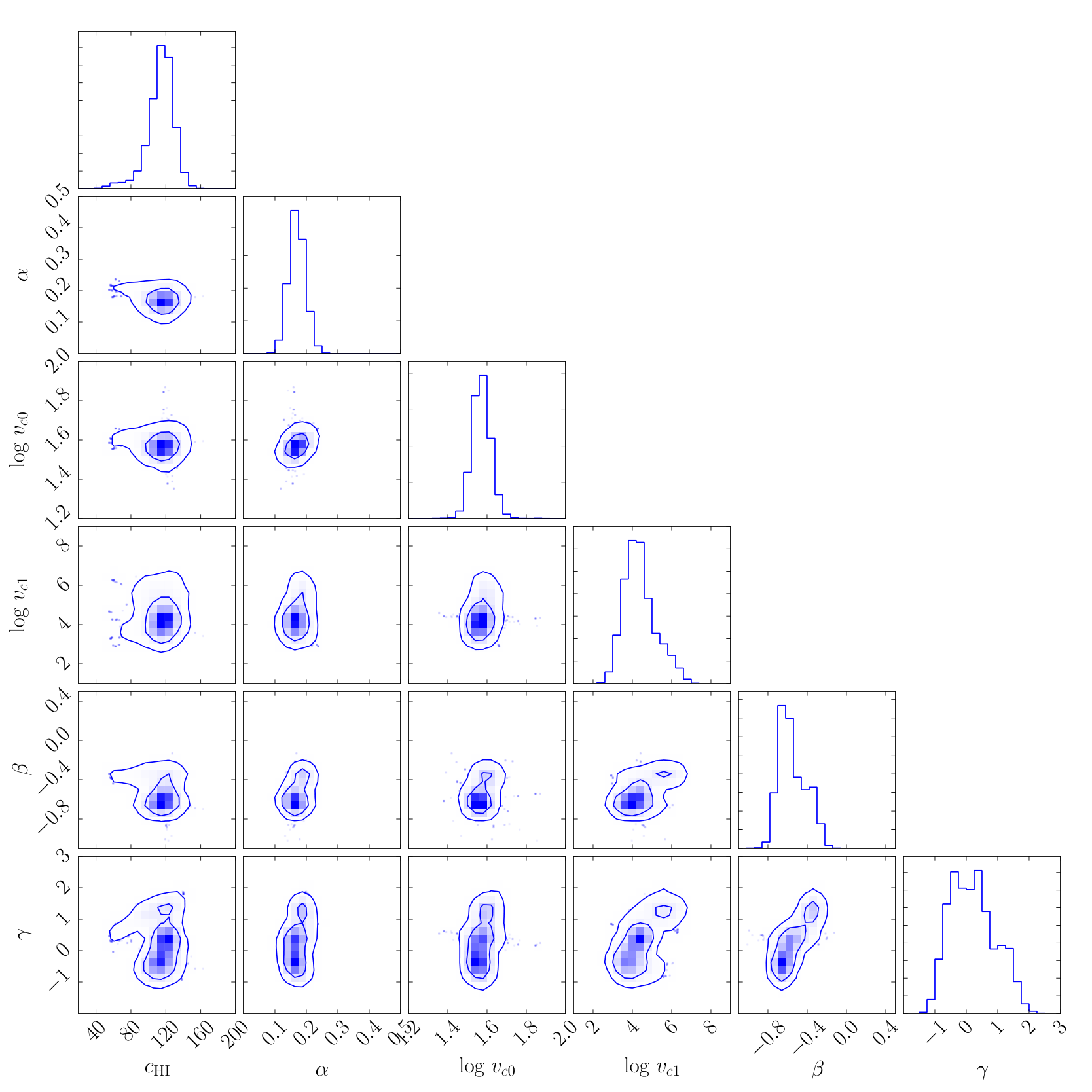
We sample the likelihood using 100 chains each of 10 random walkers for each of the 6 parameters, making a total of 6000 chains. 44 4 We find the likelihood to be adequately converged for the above number of iterations. For computational efficiency, we restrict the fitting of the column density distribution to column densities upto cm-2, however, since the function is monotonic with little or no structure, we find that the best-fitting model is an adequate match at higher column densities as well. The best-fitting values and the uncertainties so derived for the parameters are in the last two columns of Table 1. For the quoted best-fit values and errors, we use the mean and uncertainties of the values from the MCMC analysis.
A comparison of the best-fit model to the data is provided in the panels of Figs. 1, 2 and 3, for the redshifts 0, 1 and 2.3 respectively. The bands and error bars show the observables predicted by the best-fitting model with the mean values for the six parameters. The uncertainties are determined by propagating the errors in the parameters in quadrature. Most of the observables are fairly well fit by the model predictions, apart from an under prediction of at (also seen in the previous study, Paper 2). There are also indications of a possible tension between the mass function of Hi-selected galaxies and the column density distribution at . Note that, at low redshifts, the systematic uncertainties in the reported measurements of the column density distribution and the mass function may be significant compared to the statistical uncertainties. To provide an indicative measure of the systematic effects, we have plotted multiple measurements where available, for example, the Braun (2012) and the Zwaan et al. (2005b) measurements of the column density distribution, and the Zwaan et al. (2005a) and Martin et al. (2010) measurements of the mass function at . To explore the possibility of the observed tension being alleviated by the systematics in the measurements at , especially in the case of , we repeat the analysis with the Braun (2012) data (in place of the WHISP data) in the Appendix. We find, as a result of this analysis, that the systematics in the data may not fully alleviate the observed tension.
The posterior probabilities from the MCMC analysis, and the parameter space are shown in Fig. 4. The resultant form of at is shown in the left panel of Fig. 5, along with the results of other studies in the literature (Marín et al., 2010; Davé et al., 2013). The evolution of the relation for redshifts 0-4 is shown in the right panel of Fig. 5, along with the relation for (shown by the dashed line). It can be seen that the relation derived from the best-fitting model has a shallower slope in all cases, illustrating the effect of negative values for .
There is no redshift evolution in the present , apart from that coming from the evolution of the virial velocity to halo mass relation. A possible evolution in the parameter may be needed to match the observed clustering bias of DLAs at , which we explore in greater detail in future work. The evolution of the relation can be constrained by current and future intensity mapping experiments which measure the large-scale power spectrum . There are also studies that infer the mean host halo mass of DLA systems at high redshift through clustering and cross-correlation studies (Bouché et al., 2005; Font-Ribera et al., 2012). Cross-correlations of the 21-cm intensity maps with a large sample of optical galaxies (Chang et al., 2010; Masui et al., 2013; Switzer et al., 2013, e.g.) can potentially provide powerful constraints on the Hi-halo mass relation.
Finally, we plot the model predictions for the evolution of the bias, both for Hi and DLAs, and the incidence as a function of redshift. The errors on these are again determined by propagating in quadrature the uncertainties in the free parameters. These predictions are shown along with the data points in Figs. 6 and 7 respectively. The predictions for at intermediate and high redshifts are important in the context of current and upcoming intensity mapping experiments.
We thus find that the additional input of the Hi mass function at low-, constrains the value of to less than zero, thereby making the logarithmic slope of the Hi-halo mass relation lower than unity. This slope is directly related also to the high-mass cutoff in the Hi-halo mass relation (the value of ). A smaller slope allows a higher value of to be consistent with the measurements, since it results in a lower weight being given to the high mass end of the Hi-halo mass relation. We thus see that the introduction of the parameter is essential for obtaining a good fit to the low-redshift Hi mass function and contributes towards constraining the overall "shape" of the Hi-halo mass relation.
The parameter , used in the redshift evolution of the Hi profile, is also found to converge to a value less than unity. This quantifies the redshift evolution of the Hi concentration parameter compared to that expected from dark matter alone. If we define an "effective" concentration parameter , we thus find evidence for a non-trivial redshift evolution of the , with the remaining evolution in the profile being identical to that of the dark matter. This evolution of the effective concentration of Hi is shown in Fig. 8 with its error band, which indicates a mild increase of the best-fitting Hi concentration with increasing redshift.
5 Conclusions
In this paper, we have carried out a detailed statistical study of the evolution of Hi across redshifts by utilizing all the available data, both from the 21-cm based as well as the DLA-based observables. We build upon the results of our previous fitting to the observations (Paper 2) by generalizing the form of and the Hi profile from older analyses, thus introducing extra degrees of freedom. We thus explore how well we can use the data available at present to develop a halo-model based approach towards analyzing Hi. The model free parameters are constrained using a full MCMC analysis so that the posterior distributions and the correlations between parameters can be effectively explored. We find that a model which is reasonably consistent with all available data underpredicts the value of DLA bias at , as shown in Figs. 3 and 6. This was also observed with the previous fitting analysis (Paper 2). The model predictions are nevertheless consistent with the results of DLA imaging studies, which favour the association of high-redshift DLAs with faint dwarf galaxies (Cooke et al., 2015; Fumagalli et al., 2014; Fumagalli et al., 2015), and the results of hydrodynamical simulations (Rahmati & Schaye, 2014; Davé et al., 2013, e.g.,).
The introduction of the new parameters and constrains the shape of the Hi-halo mass relation and also the form and evolution of the Hi density profile. Constraining results in a smaller weight being given to the higher range of host halo masses, thus allowing the upper cutoff to be higher than for the case with . It is also seen from the results of abundance matching (Papastergis et al., 2013) that a flatter relation is favoured by the observations of ALFALFA Hi galaxies. However, there are indications of a possible tension between the Hi column density distribution and the mass function of Hi-selected galaxies at . This tension may not be fully alleviated by the systematic effects in the measurements of the column density distribution and the mass function at . It is possible that the form of the profile at low redshifts needs to be modified in order to fit the observed column density distribution. We hope to consider other forms of the profile such as an exponential surface density profile, as well as a possible variation of the form of the profile across redshifts in future work.
With the introduction of the parameter , the redshift evolution of the concentration can be effectively explored, and it can be seen that a mild increase in Hi concentration with redshift is favoured by the best-fitting model.
In future work, it would be interesting to extend the results of this halo model framework to include small-scale clustering, measured from surveys of Hi selected galaxies and DLA systems.This serves to provide additional constraints on the profile parameters, as well as their evolution across redshifts. This extension would also enable comparison to the results of hydrodynamical simulations, and thus shed light on the connections between Hi and galaxy evolution over cosmic time. Finally, such a combined halo model would have important consequences for constraining the expected signal in the Hi power spectrum, to be measured with current and future intensity mapping experiments.
Acknowledgements
We thank Tirthankar Roy Choudhury, Adam Amara, Phil Bull, Girish Kulkarni, Supratik Pal, Sebastian Seehars and Ali Rahmati for useful discussions and comments on the manuscript, and Joel Akeret for help and support with the CosmoHammer package. We thank the anonymous referee for a detailed and helpful report that improved the content and presentation. The research of HP is supported by the Tomalla Foundation.
References
- Akeret et al. (2013) Akeret J., Seehars S., Amara A., Refregier A., Csillaghy A., 2013, Astronomy and Computing, 2, 27
- Bagla et al. (2010) Bagla J. S., Khandai N., Datta K. K., 2010, MNRAS, 407, 567
- Barnes & Haehnelt (2010) Barnes L. A., Haehnelt M. G., 2010, MNRAS, 403, 870
- Barnes & Haehnelt (2014) Barnes L. A., Haehnelt M. G., 2014, MNRAS, 440, 2313
- Bird et al. (2014) Bird S., Vogelsberger M., Haehnelt M., Sijacki D., Genel S., Torrey P., Springel V., Hernquist L., 2014, MNRAS, 445, 2313
- Bouché et al. (2005) Bouché N., Gardner J. P., Katz N., Weinberg D. H., Davé R., Lowenthal J. D., 2005, ApJ, 628, 89
- Braun (2012) Braun R., 2012, ApJ, 749, 87
- Bull et al. (2015) Bull P., Ferreira P. G., Patel P., Santos M. G., 2015, ApJ, 803, 21
- Chang et al. (2008) Chang T.-C., Pen U.-L., Peterson J. B., McDonald P., 2008, Physical Review Letters, 100, 091303
- Chang et al. (2010) Chang T.-C., Pen U.-L., Bandura K., Peterson J. B., 2010, Nature, 466, 463
- Cooke et al. (2015) Cooke R. J., Pettini M., Jorgenson R. A., 2015, ApJ, 800, 12
- Crighton et al. (2015) Crighton N. H. M., et al., 2015, MNRAS, 452, 217
- Davé et al. (2013) Davé R., Katz N., Oppenheimer B. D., Kollmeier J. A., Weinberg D. H., 2013, MNRAS, 434, 2645
- Font-Ribera et al. (2012) Font-Ribera A., et al., 2012, J. Cosmology Astropart. Phys., 11, 59
- Fumagalli et al. (2011) Fumagalli M., Prochaska J. X., Kasen D., Dekel A., Ceverino D., Primack J. R., 2011, MNRAS, 418, 1796
- Fumagalli et al. (2014) Fumagalli M., O’Meara J. M., Prochaska J. X., Kanekar N., Wolfe A. M., 2014, MNRAS, 444, 1282
- Fumagalli et al. (2015) Fumagalli M., O’Meara J. M., Prochaska J. X., Rafelski M., Kanekar N., 2015, MNRAS, 446, 3178
- Guha Sarkar et al. (2012) Guha Sarkar T., Mitra S., Majumdar S., Choudhury T. R., 2012, MNRAS, 421, 3570
- Hall et al. (2013) Hall A., Bonvin C., Challinor A., 2013, Phys. Rev. D, 87, 064026
- Kim et al. (2016) Kim H.-S., Wyithe J. S. B., Baugh C. M., Lagos C. d. P., Power C., Park J., 2016, preprint, (arXiv:1603.02383)
- Lanzetta et al. (1991) Lanzetta K. M., Wolfe A. M., Turnshek D. A., Lu L., McMahon R. G., Hazard C., 1991, ApJS, 77, 1
- Macciò et al. (2007) Macciò A. V., Dutton A. A., van den Bosch F. C., Moore B., Potter D., Stadel J., 2007, MNRAS, 378, 55
- Maller & Bullock (2004) Maller A. H., Bullock J. S., 2004, MNRAS, 355, 694
- Marín et al. (2010) Marín F. A., Gnedin N. Y., Seo H.-J., Vallinotto A., 2010, ApJ, 718, 972
- Martin et al. (2010) Martin A. M., Papastergis E., Giovanelli R., Haynes M. P., Springob C. M., Stierwalt S., 2010, ApJ, 723, 1359
- Martin et al. (2012) Martin A. M., Giovanelli R., Haynes M. P., Guzzo L., 2012, ApJ, 750, 38
- Masui et al. (2013) Masui K. W., et al., 2013, ApJ, 763, L20
- Navarro et al. (1997) Navarro J. F., Frenk C. S., White S. D. M., 1997, ApJ, 490, 493
- Noterdaeme et al. (2012) Noterdaeme P., et al., 2012, A&A, 547, L1
- Obreschkow et al. (2009) Obreschkow D., Klöckner H.-R., Heywood I., Levrier F., Rawlings S., 2009, ApJ, 703, 1890
- Padmanabhan et al. (2015) Padmanabhan H., Choudhury T. R., Refregier A., 2015, MNRAS, 447, 3745
- Padmanabhan et al. (2016) Padmanabhan H., Choudhury T. R., Refregier A., 2016, MNRAS, 458, 781
- Papastergis et al. (2013) Papastergis E., Giovanelli R., Haynes M. P., Rodríguez-Puebla A., Jones M. G., 2013, ApJ, 776, 43
- Pontzen et al. (2008) Pontzen A., et al., 2008, MNRAS, 390, 1349
- Prochaska & Wolfe (2009) Prochaska J. X., Wolfe A. M., 2009, ApJ, 696, 1543
- Rahmati & Schaye (2014) Rahmati A., Schaye J., 2014, MNRAS, 438, 529
- Rao et al. (2006) Rao S. M., Turnshek D. A., Nestor D. B., 2006, ApJ, 636, 610
- Santos et al. (2015) Santos M., Alonso D., Bull P., Silva M. B., Yahya S., 2015, Advancing Astrophysics with the Square Kilometre Array (AASKA14), p. 21
- Scoccimarro et al. (2001) Scoccimarro R., Sheth R. K., Hui L., Jain B., 2001, ApJ, 546, 20
- Sheth & Tormen (2002) Sheth R. K., Tormen G., 2002, MNRAS, 329, 61
- Switzer et al. (2013) Switzer E. R., et al., 2013, MNRAS, 434, L46
- Villaescusa-Navarro et al. (2015) Villaescusa-Navarro F., Bull P., Viel M., 2015, ApJ, 814, 146
- Wang et al. (2014) Wang J., et al., 2014, MNRAS, 441, 2159
- Zafar et al. (2013) Zafar T., Péroux C., Popping A., Milliard B., Deharveng J.-M., Frank S., 2013, A&A, 556, A141
- Zwaan et al. (2005a) Zwaan M. A., Meyer M. J., Staveley-Smith L., Webster R. L., 2005a, MNRAS, 359, L30
- Zwaan et al. (2005b) Zwaan M. A., van der Hulst J. M., Briggs F. H., Verheijen M. A. W., Ryan-Weber E. V., 2005b, MNRAS, 364, 1467
Appendix A Impact of systematic uncertainties on the fitted parameters
In this appendix, we provide an indicative measure of the impact of systematic uncertainties in the measurement of the column density distribution at by repeating the analysis in the main text for the Braun (2012) data. The resulting corner plot is shown by the green curves in Fig. 9 and is overplotted on the corresponding corner plot in the main text (shown in blue). The comparison to the analysis in the main text is summarized in the first four columns of Table 2.
| Parameter | Best fit (WHISP) | Error (1; WHISP) | Best fit (Braun) | Error (1; Braun) | Best fit (combined) | Error (1; combined) |
|---|---|---|---|---|---|---|
| 113.80 | 14.03 | 128.05 | 12.63 | 123.79 | 15.67 | |
| 0.17 | 0.02 | 0.16 | 0.01 | 0.16 | 0.02 | |
| log (km/s) | 1.57 | 0.03 | 1.61 | 0.03 | 1.61 | 0.05 |
| log (km/s) | 4.39 | 0.75 | 4.93 | 0.68 | 4.64 | 0.72 |
| -0.55 | 0.12 | -0.66 | 0.06 | -0.63 | 0.07 | |
| 0.22 | 0.67 | 0.55 | 0.20 | 0.58 | 0.37 |
An indicative measure of the systematic effects can also be provided by considering the difference between two observational datasets to provide an estimate of systematic errors. We consider the effect of using the difference between the two column density distribution measurements (from the WHISP and Braun (2012)), and also the two mass function measurements (from HIPASS; Zwaan et al. (2005a) and ALFALFA; Martin et al. (2010)) as measures of the systematic uncertainties in the observables. The systematic uncertainty in each case is then added to the statistical uncertainty in quadrature. Upon repeating the analysis, we find the best-fit parameters given by the fifth and sixth columns of Table 2. The best-fit parameter values for the three analyses are consistent within , indicating that systematic effects may not be completely responsible for the observed tension between the column density and the Hi mass function.