Thermodynamics and renormalized quasi-particles in the vicinity of the dilute Bose gas quantum critical point in two dimensions

At finite chemical potential $\mu$ and temperature $T=1/\beta$, the Euclidean action associated with the Hamiltonian (2) can be written as

where the free boson propagator is

and we have introduced the composite boson fields

Here $K=(\bm{k},i\omega)$ and $P=(\bm{p},i\bar{\omega})$ are collective labels for momenta and bosonic Matsubara frequencies, the integration symbols are defined by $\int_{K}=\frac{1}{\beta V}\sum_{\bm{k},\omega}$, and $a_{K}$ is a complex field associated with the eigenvalues of $\hat{a}_{\bm{k}}$. Introducing another complex boson field $\psi_{P}$ to decouple the interaction by means of a Hubbard-Stratonovich (HS) transformation in the particle-particle channel we obtain

We have normalized the $\psi$-field to simplify the combinatorial factors in the exact FRG flow equations given in appendix A. Below we shall refer to the original boson fields $a$ and $\bar{a}$ as elementary bosons and to the boson fields $\psi$ and $\bar{\psi}$ as HS bosons.

To set up the FRG, we introduce a sharp cutoff in momentum space for the elementary boson so that the regularized non-interacting propagator is given by

and the corresponding single-scale propagator is

where $\Sigma_{\Lambda}(K)$ is the cutoff dependent self-energy and we have defined $\xi_{\bm{k}}=\epsilon_{\bm{k}}-\mu$. For our purpose, it is sufficient to use the following ansatz for the generating functional of the irreducible vertices,

where the energy-momentum labels of the three-legged vertices $\Gamma_{\Lambda}^{\bar{a}\bar{a}\psi}(P-K,K;P)$ and $\Gamma_{\Lambda}^{{a}{a}\bar{\psi}}(P-K,K;P)$ correspond to the field types appearing in the superscripts. This ansatz is justified since all four-point and higher order vertices are irrelevant in the RG sense, except for $\Gamma_{\Lambda}^{\bar{a}\bar{a}aa}$ which is marginal. This vertex, however, initially vanishes due to the HS transformation and is only dynamically generated during the flow by either particle-hole processes or by vertices which are irrelevant in the RG sense (see Fig. 13). As our calculations are concerned with the dilute limit, particle-hole processes are suppressed and the relevant physics is captured by particle-particle processes via the three-point vertices $\Gamma_{\Lambda}^{\bar{a}\bar{a}\psi}$ and $\Gamma_{\Lambda}^{{a}{a}\bar{\psi}}$. The exact FRG flow equations for the self-energy $\Sigma_{\Lambda}(K)$ and the particle-particle susceptibility $\Pi_{\Lambda}(P)$ as well as for all three- and four-legged vertices of our model are given in appendix A. From the flow equations (74) and (75) for the three-legged vertices we see that within our ansatz (9) for the generating functional these vertices do not flow, so that we can replace them by their initial value

The exact flow equation for the self-energy given in Eq. (72) then simplifies to

while the flow equation for the particle-particle susceptibility given in Eq. (73) becomes

Here we have introduced the flowing propagator

of the HS boson. We expect these equations to be accurate in the vicinity of the dilute Bose gas QCP where particle-hole scattering processes can be neglected.

Note that if we replace the single-scale propagators in Eqs. (11) and (12) by total derivatives with respect to $\Lambda$ and ignore the $\Lambda$ dependence of the particle-particle susceptibility $\Pi_{\Lambda}$, we can integrate both sides of these equations over $\Lambda$ to obtain

These coupled integral equations are usually called the self-consistent $T$-matrix approximation. For an early application of this method to the dilute Bose gas in two dimensions see Ref. [30]. Some of us [31] have recently used this approximation to study an effective hard-core boson model describing the magnetic properties of the antiferromagnetic material $\text{Cs}_{2}\text{CuCl}_{4}$ (see also Ref. [32] for recently discovered subtleties in this method when applied to hard-core bosons). In Sec. V.1 we shall compare our FRG results for the wavefunction renormalization at $\mu=0$ to the results obtained from the numerical solution of the integral equations (14) and (15).

To begin with, let us briefly recall the renormalization group (RG) flow of the system directly at the QCP in $D$ dimensions. Since in this case the equilibrium state of the system corresponds to the vacuum, the elementary propagator $G_{\Lambda}(K)$ is identical to the free propagator $G_{0,\Lambda}(K)$, i.e., $\Sigma_{\Lambda}(K)=0$. According to Eqs. (11) and (12) the flow of the particle-particle susceptibility for vanishing momentum and frequency then simplifies to

where $K_{D}$ is the surface area of the $D$-dimensional unit sphere divided by $(2\pi)^{D}$. Defining the dimensionless rescaled interaction

and switching to the logarithmic scale parameter $l=\ln(\Lambda_{0}/\Lambda)$, where $\Lambda_{0}$ is the ultraviolet cutoff of our theory, we arrive at the well-known exact flow equation[20, 1]

which identifies $D_{c}=2$ as the upper critical dimension above which mean field theory is applicable. In the following we will always work at $D=D_{c}$, resulting in logarithmic corrections to the scaling of various observables.

The above system of FRG flow equations (11) and (12) for the self-energy and the particle-particle susceptibility can be solved approximately by neglecting their momentum and frequency dependence which is justified close to the QCP. In the following we will again use the scaling parameter $l=\ln(\Lambda_{0}/\Lambda)$ and the dimensionless interaction

which is a special case of Eq. (17) for $D=2$. We also define the effective inverse temperature

the dimensionless particle-particle susceptibility

and the effective negative chemical potential over temperature

where we have introduced the abbreviation

to simplify the forthcoming equations. With this notation the flow equations (11) and (12) can be written as

It turns out that we can analytically solve this system of differential equations approximately for $r=\lim_{l\rightarrow\infty}r_{l}$ provided we consider the regime close to the QCP and the following dimensionless coupling is sufficiently small,

where the logarithmic term results from the flow of $\tilde{\Pi}_{l}$ [cf. Eq. (84)]. Technical details on the analytical solution of Eqs. (24) and (25) are given in appendix B.1. There we show that an approximate analytical solution is possible if either $g\ll\alpha$ or $W(1/g)\gg 1$, where $W(x)$ denotes the Lambert W function [33] which for large arguments can be expanded as

The condition $W(1/g)\gg 1$ is thus fulfilled either extremely close to the QCP or for small bare interaction $u_{0}$. The regime $u_{0}\ll 1$ is of significant practical importance as it allows to probe the asymptotic scaling behavior experimentally by tuning the interaction to small values, since reaching double exponentially low temperatures is not feasible. Actually for small $u_{0}$ the weak logarithmic dependence on $T$ results in an approximate temperature independence of $g$.

As shown in appendix B.1, for $\mu\leq 0$ the limit $r=\lim_{l\rightarrow\infty}r_{l}$ can be written as

which in the special case $\mu=0$ simplifies to

On the other hand, for finite $\alpha>0$ and $g\ll 1$ we can expand Eq. (28) as

which in the quantum disordered regime where $\alpha\gg 1$ results in

so that the self-energy is exponentially suppressed.

In appendix B.1 we also derive a more general expression,

which is valid for arbitrary $\alpha=-\mu/T$ as long as we stay in the normal phase close to the QCP and do not come too close to the BKT phase transition. The reason for the latter constraint is that vortices become increasingly important close to the superfluid transition which eventually leads to a breakdown of the quasi-particle approximation $\Sigma(K)\approx\Sigma(0)$ (cf. Fig. 9 at $\mu>0$). Nevertheless, extrapolating (32) into the classical critical regime we can give an estimate for the critical chemical potential $\mu_{c}$ at the BKT transition by demanding that $r=0$, which in the asymptotic limit yields

Given that our theory is not justified in the classical critical regime, this agrees well with the weak-coupling result [34, 20]

where $C_{\mu}$ has been obtained numerically as $C_{\mu}\approx 4.2$ in Ref. [22] and as $C_{\mu}\approx 3.0$ in Ref. [26].

Within our approximation scheme the density at scale $\Lambda$ is given by

which corresponds to the particle density of all particles with momentum $k>\Lambda$. The integration can be carried out exactly and we obtain for the physical density

Analogously the off-diagonal elements of the density matrix in our approximation are

In the limit of large distances $|\bm{x}-\bm{x}^{\prime}|\to\infty$ and for $\Lambda\to 0$ we can evaluate the momentum integration analytically,[29]

where we have introduced the correlation length

We now define the reduced pressure $\tilde{p}$, the phase-space density $\tilde{n}$, the entropy per particle $\tilde{s}$, the dimensionless compressibility $\tilde{\kappa}$, and the dimensionless correlation length $\tilde{\xi}$,

where $p$ is the pressure, $\Omega$ is the grand canonical potential, $S$ is the entropy, $\kappa=\left(\partial n/\partial\mu\right)_{T}$ is the compressibility, and the thermal de Broglie wavelength is given by

Since we have approximated the self-energy by its zero momentum and frequency limit, we can try to incorporate the interaction solely as a shift in the chemical potential, neglecting the renormalized interaction $u$. Thus we compute the state functions for a non-interacting Bose gas and fix the chemical potential such that the particle density $n_{\text{free}}$ coincides with Eq. (36), i.e., $\mu_{\text{free}}=\mu-\Sigma(0)$. Accordingly we find

where $\text{Li}_{2}(x)$ is the dilogarithm. Calculating the dimensionless compressibility from Eq. (42b) yields

We note that these observables do not have a well-defined limit at $\mu=T=0$ due to the non-analyticity of the grand canonical potential at the QCP, which separates the zero density ground state at $\mu<0$ from the finite density superfluid ground state at $\mu>0$. For the special case of vanishing chemical potential the above relations have already been obtained by Rançon and Dupuis [26] whose results agree with our expressions for $\mu=0$.

Note that Eq. (42b) corrects the result for the density at $\mu=0$ given by Sachdev et al.,[21]

while we find from Eqs. (42b) and (26)

We can improve on the calculation of $\tilde{p}$ and $\tilde{s}$ by directly calculating the grand canonical potential within the FRG formalism, solving the flow equation

Allowing for first order corrections in the self-energy,

the flow equation for the reduced pressure $\tilde{p}=-\frac{\lambda_{\text{th}}^{2}}{T}\frac{\Omega}{V}$ reads within our cutoff scheme (see appendix B.2)

Approximating $Z_{l}=Y_{l}=1$ and $r_{l}=r$ results in $\tilde{p}=\text{Li}_{2}(e^{-r})$ which agrees with the reduced pressure in Eq. (42a). In contrast, if we solve the flow equation (48) for $\tilde{p_{l}}$ at $\mu=0$ with the flowing $r_{l}$ we find (see appendix B.3)

Here the leading correction is only half as large as our earlier result in Eq. (42a). This implies that it is necessary to solve the flow equation for the grand canonical potential to obtain the correct leading order scaling behavior for the reduced pressure. The entropy per particle, which at $\mu=0$ can be derived from the reduced pressure as

is only affected to subleading order. While the phase-space density can in principle also be calculated from $\tilde{p}$ as $\tilde{n}=\partial\tilde{p}/\partial(\mu/T)_{T}$, it is preferable to use Eq. (36) as it avoids the additional approximations in the computation of the reduced pressure.

In Fig. 2 we compare our results for the thermodynamic state functions at $\mu=0$ (solid black and dashed blue lines) with empirical data from three ultra-cold atoms experiments (green symbols) which we call Chicago I,[14] ENS,[15] and Chicago II,[16] following the naming introduced in Ref. [26]. The first two experiments investigated $\hphantom{{}^{\mathrm{133}}_{\mathrm{}}}{\vphantom{\mathrm{X}}}{}^{\mathchoice{\hbox to0.0pt{\hss$\displaystyle\vphantom{\smash[t]{\mathrm{2}}}\mathrm{133}$}}{\hbox to0.0pt{\hss$\textstyle\vphantom{\smash[t]{\mathrm{2}}}\mathrm{133}$}}{\hbox to0.0pt{\hss$\scriptstyle\vphantom{\smash[t]{\mathrm{2}}}\mathrm{133}$}}{\hbox to0.0pt{\hss$\scriptscriptstyle\vphantom{\smash[t]{\mathrm{2}}}\mathrm{133}$}}}\kern 0.0pt\mathrm{Cs}$ and $\hphantom{{}^{\mathrm{87}}_{\mathrm{}}}{\vphantom{\mathrm{X}}}{}^{\mathchoice{\hbox to0.0pt{\hss$\displaystyle\vphantom{\smash[t]{\mathrm{2}}}\mathrm{87}$}}{\hbox to0.0pt{\hss$\textstyle\vphantom{\smash[t]{\mathrm{2}}}\mathrm{87}$}}{\hbox to0.0pt{\hss$\scriptstyle\vphantom{\smash[t]{\mathrm{2}}}\mathrm{87}$}}{\hbox to0.0pt{\hss$\scriptscriptstyle\vphantom{\smash[t]{\mathrm{2}}}\mathrm{87}$}}}\kern 0.0pt\mathrm{Rb}$ atoms, respectively, inside a harmonic potential with strong confinement along the $z$-axis, resulting in a quasi two-dimensional system; connection to homogeneous systems was made through the local density approximation. While the 3D scattering length in Ref. [15] was fixed at $a=5.3$ nm ($g=0.035$), the Chicago I experiment used a magnetic Feshbach resonance to vary $a$ between $2-10$ nm ($g=0.016-0.083$). These values of $g$ correspond to $W(1/g)=1.9-3.0$ which is not much larger than unity, in contrast to the assumption in our calculations; nevertheless we find that the agreement between the analytical results and the aforementioned experiments is quite good. On the other hand the measurements from the Chicago II experiment, based on $\hphantom{{}^{\mathrm{133}}_{\mathrm{}}}{\vphantom{\mathrm{X}}}{}^{\mathchoice{\hbox to0.0pt{\hss$\displaystyle\vphantom{\smash[t]{\mathrm{2}}}\mathrm{133}$}}{\hbox to0.0pt{\hss$\textstyle\vphantom{\smash[t]{\mathrm{2}}}\mathrm{133}$}}{\hbox to0.0pt{\hss$\scriptstyle\vphantom{\smash[t]{\mathrm{2}}}\mathrm{133}$}}{\hbox to0.0pt{\hss$\scriptscriptstyle\vphantom{\smash[t]{\mathrm{2}}}\mathrm{133}$}}}\kern 0.0pt\mathrm{Cs}$ atoms in a two-dimensional optical lattice, differ visibly from our predictions for $\tilde{p}$ and $\tilde{s}$ which is not surprising given that $g=0.68$ is relatively large, while the agreement for $\tilde{n}$ is still remarkably good.

As a further benchmark we use the results of Rançon and Dupuis[26] (dash-dotted red lines) who numerically computed the state functions within the FRG using a truncated gradient expansion. We find that the plots for the phase-space density $\tilde{n}$ essentially agree, while the reduced pressure $\tilde{p}$ and the entropy per particle $\tilde{s}$ differ for $g\gtrsim 0.1$. This indicates the upper boundary of the regime where our asymptotic analysis is valid for these state functions.

The magnetization data from the simulations follows a characteristic finite-size scaling of the form $M(L)/N=M(\infty)/N+b\,\exp(-L/\xi^{\prime})$, where $b$ and $\xi^{\prime}$ are temperature dependent as will be discussed in more detail in Sec. IV.3. Basically the finite-size correlation length $\xi^{\prime}$ decreases with increasing temperature up to some temperature $T_{\rm end}$, above which the data becomes largely independent of $L$ for the system sizes used. In Fig. 3 we show the QMC results with error bars (black) for the density over temperature as a function of $T$ in the thermodynamic limit at the lower critical field $B=-2J$, corresponding to a vanishing chemical potential $\mu=0$. The solid line (blue) is a fit using Eq. (36) together with Eq. (32) in the limit $1/u_{0}\to 0$ for hard-core bosons. Keeping both $m$ and $\Lambda_{0}$ as fitting parameters we obtain the expected result $mJ=1$ within a few percent. Setting $mJ=1$ for simplicity and using only the ultraviolet cutoff $\Lambda_{0}$ as a fitting parameter, we obtain $\Lambda_{0}=23.5\pm 1.5$ where we have required that the deviation between our analytical result and the QMC data vanishes in the limit $T\to 0$ (see inset of Fig. 3).

For comparison we also tested the leading order expression for the density given in Eq. (45) using the same cutoff $\Lambda_{0}=23.5$, which predicts $n/T$ to be more than $40\%$ below the QMC data for the temperatures used here. It is possible to use a rather different cutoff $\Lambda_{0}\approx 205$ and a modified mass $mJ\approx 0.8$ to fit the leading order expression in Eq. (45) to the QMC data as shown by the dashed line (red) in Fig. 3. It seems that such a fit compensates higher order corrections by using a modified effective mass and a large value of the cutoff. In turn this means that for most experimental and numerical data the coupling constant $g$ is sufficiently small to guarantee that the approximate solution in Eq. (36) is accurate, but $g$ is not exponentially small to justify dropping all higher order terms (see $g$-axes in Fig. 3 and Fig. 4). Therefore, a fit to the simple logarithmic behavior in Eq. (45) may yield an incorrect cutoff and mass to compensate different higher order corrections. In the temperature region around the minimum in Fig. 3 the scaling of the density may even appear perfectly linear with temperature, which is consistent with recent results on two-dimensional coupled spin-dimers systems.[28]

The corresponding data for the compressibility is shown in Fig. 4. The same form of the finite-size scaling was used, but it should be noted that convergence to the thermodynamic limit requires larger system sizes for this response function. Using Eq. (40d) and the analytic expression in Eq. (43) we find good agreement using again $mJ=1$, but a larger cutoff $\Lambda_{0}=31\pm 2$. Note that the effective coupling $g$ in Eq. (26) depends only logarithmically on $\Lambda_{0}$ so that the difference in the cutoffs only results in a rather small correction. Nevertheless we find that we cannot choose a single cutoff to fit our analytical results for both the density and the compressibility to the QMC data. We have checked the size-scaling for the particle density as well as for the compressibility very carefully, so that we can be sure that the deviation in the cutoff is not related to any remaining finite-size effects. Instead, the different values of $\Lambda_{0}$ might be due to the fact that the condition $g\ll 1$, requiring exponentially low temperatures due to the hard-core interaction, is not strictly fulfilled in the accessible temperature regime (see Fig. 3 and Fig. 4). Hence we would expect that our analytical result (32) is only qualitatively correct and we need different values of the cutoff for quantitative agreement with the QMC simulations.

Next, let us consider the regime of constant, non-zero $\alpha=-\mu/T>0$, corresponding to approaching the QCP diagonally from the left in the $\mu$-$T$-diagram shown in Fig. 1. We investigate a wide range of values for $\alpha$, starting from $0.1$ up to $2.0$.

The QMC data (solid and open symbols) for the density and the compressibility at $\alpha=0.1$ are shown in Fig. 5 as a function of temperature, where we compare them to our analytical results in Eqs. (36) and (40d) (solid lines). The fit for the density shows good agreement for $mJ=1$ and $\Lambda_{0}=23\pm 2$ (upper green line), which is consistent with the estimate for $\mu=0$ from above. For the compressibility we find good agreement using $mJ=1$ and $\Lambda_{0}=27.5\pm 2$ (upper red line). It should be noted that it is again possible to fit the data to a leading order expansion of our analytical results, but this leads to values for the cutoff which are even larger than in the case of $\alpha=0$.

Increasing $\alpha$ to $0.4$ as shown in Fig. 5 (lower graphs), we see that the magnitude of the density and the compressibility is lowered, but the overall shape is similar. Compared to the case $\alpha=0$ the value of the respective cutoffs decreases, $\Lambda_{0}=21\pm 2$ for the density and $\Lambda_{0}=20\pm 2$ for the compressibility at $\alpha=0.4$, while at the same time the difference between the two cutoffs becomes negligible within errors.

Monte Carlo results for $\alpha=1$ and $\alpha=2$ are presented in Fig. 6; with increasing $\alpha$, the temperature region for which we can apply the fit functions is pushed to lower and lower values of $T$, while at the same time the characteristic minimum in $n/T$ at $T_{\text{min}}$ is shifted to lower temperatures as well. Note that $\kappa$ also shows a minimum at slightly larger temperatures which does not shift as much with $\alpha$, so that both minima approach each other for $\alpha=2$. Remarkably, both $\kappa$ and $n/T$ take on the same value at a certain crossing temperature of $T=0.0228\pm 0.0018$ (QMC) or $T=0.018\pm 0.003$ (fits), which is largely independent of $\alpha$.

From the fits of the density the cutoff can be consistently estimated to be in the range $\Lambda_{0}\approx 22\pm 2$ for all values of $\alpha$. The data for the compressibility at small $\alpha$ gives slightly larger estimates for $\Lambda_{0}$, indicating that in this case our analytical results for $\kappa$ require smaller values of $g$ than for the density. This is consistent with Fig. 2 where we find good agreement with Ref. [26] for $n/T$ in a surprisingly large regime of $g$, while our results for the other observables only agree up to $g\lesssim 0.1$.

As already mentioned before, the size scaling of the magnetization and of the susceptibility has the form

up to a characteristic temperature $T_{\text{end}}$, above which the data is mainly independent of $L$ so that a simple linear extrapolation suffices. With these fits we can extract a finite-size correlation length $\xi^{\prime}$ from the size scaling of the magnetization, which is shown in Fig. 7 for different $\alpha$ as a function of temperature using the rescaling $\xi=1.15\xi^{\prime}$. Within error bars the behavior of $\xi^{\prime}$ is consistent with the divergence $\xi\propto 1/\sqrt{T}$ in Eq. (39) for all $\alpha$. For comparison we show the analytic result from Eq. (32) for $\sqrt{T}\xi=1/\sqrt{2mr}$ as solid lines for different values of $\alpha$. The correlation length $\xi^{\prime}$ from the finite-size scaling of the Monte Carlo data discussed above shows a similar scaling behavior, although finite-size scaling does not measure the correlation length directly. Choosing the cutoff as $\Lambda_{0}=22$ consistent with the fits for the density, we observe that the correlation length $\xi^{\prime}$ from QMC finite-size scaling agrees reasonably well with the analytic prediction for $\xi$ up to the rescaling $\xi=1.15\xi^{\prime}$.

The breakdown of the exponential extrapolation in Eq. (53) defines a temperature $T_{\rm end}$, which can be used to identify a region of validity for the continuum description of the $XY$ lattice model. Above this temperature the correlation length $\xi$ is of order unity so that lattice effects dominate. As can be seen in Fig. 8, this region where the continuum description holds roughly coincides with the parameter range $g<0.5$ for $\Lambda_{0}=22$ (red shaded region), which is where our analytic prediction for $n$ in (36) can be fitted to the QMC data. The values of the temperatures $T_{\rm min}$ where the minimum in $n/T$ for a given $\alpha$ occurs are also shown and are generally at significantly larger values. Note that these minima in $n/T$ correspond to linear behavior of the density with temperature, which always occurs well above the region of validity. It is remarkable that it is possible to use Eq. (36) to describe the behavior close to the QCP also for finite $\mu$ rather accurately, but as expected smaller temperatures are required for $\alpha>0$ since we then approach the QCP diagonally in the $\mu$-$T$-diagram.

From the low-energy expansion (47) of the self-energy we see that the RG flow of $Z_{\Lambda}$ is determined by

Although the flow of $Z_{\Lambda}$ modifies also the flow equations (24) and (25) for $\Sigma_{\Lambda}(0)$ and $\Pi_{\Lambda}(0)$, we shall ignore this modification since it is not expected to change the leading asymptotics close to the quantum critical point. Neglecting the Bose distribution in the flow of the particle-particle susceptibility we end up with the approximate flow equation (see appendix B.4)

Integrating this equation we find that $Z=\lim_{l\rightarrow\infty}Z_{l}$ is given by

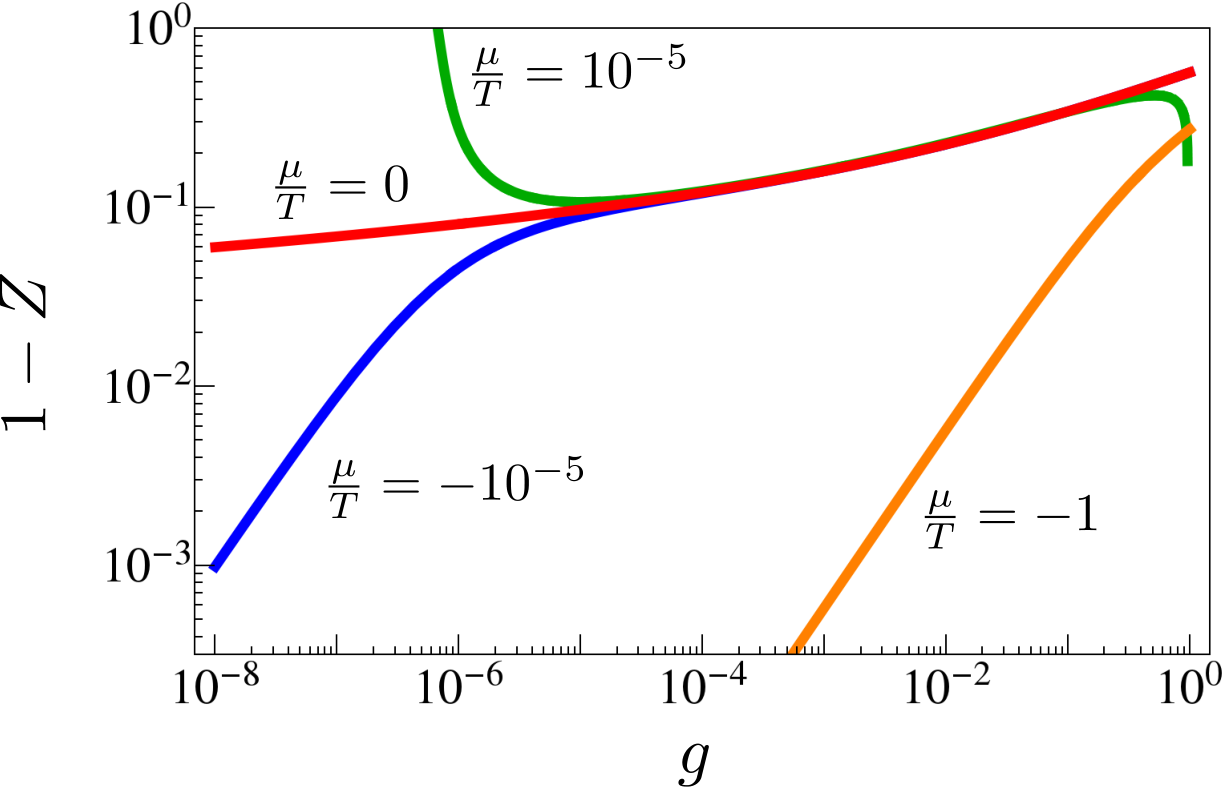
Although this result is only strictly valid for non-positive chemical potential, we find numerically that it is also qualitatively good for $\mu>0$. For vanishing chemical potential $Z$ scales as

while in the quantum disordered regime $\alpha\gg 1$ the correction is exponentially small,

We have verified the validity of these approximate expressions by solving the relevant flow equations numerically, taking the Bose distribution in the flow of $\Pi_{\Lambda}$ into account, which yields very good overall agreement. Some representative results for $1-Z$ at various values of $\mu/T$ are presented in Fig. 9. We find that for $\mu/T\leq 0$ the wavefunction renormalization approaches unity in the limit $g\to 0$ in agreement with the well-known result that $\Sigma(K)=0$ at the QCP (cf. Sec. III.1), while for positive chemical potential we have $Z=0$ at a finite $g$ where the BKT transition takes place.

Finally, we can also explore the regime of validity of the self-consistent $T$-matrix approximation as given in Eqs. (14) and (15), which in this context is expected to be good at high temperatures. On the other hand, our FRG approach should be accurate at low temperatures and it is a priori not clear whether there exists an intermediate temperature regime where both methods are valid. For simplicity we consider only the case $\mu=0$ and take the limit of infinite bare interaction, corresponding to hard-core bosons. A detailed discussion of the self-consistent $T$-matrix approach to hard-core bosons can be found in Ref. [31], where the spin Hamiltonian for the magnetic insulator $\text{Cs}_{2}\text{CuCl}_{4}$ was mapped onto a two-dimensional hard-core boson model which was then studied using the self-consistent $T$-matrix approximation.

For a comparison of this method with our FRG approach we use parameters specific to $\text{Cs}_{2}\text{CuCl}_{4}$; in particular, we choose the effective inverse temperature as $\beta_{0}=\Lambda_{0}^{2}/(2mT)\approx 1\text{K}/T$, where we have fixed the momentum cutoff $\Lambda_{0}$ to an average value of the inverse lattice parameters of $\text{Cs}_{2}\text{CuCl}_{4}$. In Fig. 10 we compare the results of both complementary methods; obviously, an intermediate temperature regime where both methods are accurate does not exist, showing the need for an alternative approach in this region. We expect that a numerical solution of the FRG flow equations (11) and (12), retaining the full momentum and frequency dependence of $\Sigma_{\Lambda}(K)$ and $\Pi_{\Lambda}(P)$, should be accurate at low as well as at high temperatures. Another possibility to describe the intermediate temperature regime is to use a lattice FRG scheme along the lines of Ref. [37].

Using Eqs. (47) and (11) we find that the flow equation for the effective mass factor $Y_{\Lambda}$ is within our truncation given by

As before we neglect the momentum dependence in the particle-particle susceptibility as well as the Bose distributions which appear in its flow equation. This allows us to compute $Y$ analytically to leading order as long as $\mu\leq 0$. For $r\ll 1$ we find

which for $\mu=0$ and small $g$ simplifies to

In the opposite regime $r\gtrsim 1$ we obtain

where the coefficient $\gamma$ is given by

Thus at $\alpha\gg 1$ the correction is again exponentially suppressed,

Representative results of $Y$ at different values of $\mu/T$ are shown in Fig. 11, which should be compared with the analogous Fig. 9 for the wavefunction renormalization factor.

References

- [1] S. Sachdev, Quantum Phase Transitions, 2nd ed. (Cambridge University Press, New York, 2011).
- [2] V. N. Popov, Theoret. and Math. Phys. 11, 565 (1972).
- [3] N. D. Mermin and H. Wagner, Phys. Rev. Lett. 17, 1133 (1966).
- [4] V. L. Berezinskii, Sov. Phys. JETP 32, 493 (1971).
- [5] V. L. Berezinskii, Sov. Phys. JETP 34, 610 (1972).
- [6] J. M. Kosterlitz and D. J. Thouless, J. Phys. C 6, 1181 (1973).
- [7] J. M. Kosterlitz, J. Phys. C 7, 1046 (1974).
- [8] M. P. A. Fisher, P. B. Weichman, G. Grinstein, and D. S. Fisher, Phys. Rev. B 40, 546 (1989).
- [9] S. Sachdev and E. R. Dunkel, Phys. Rev. B 73, 085116 (2006).
- [10] Z. Hadzibabic, P. Krüger, M. Cheneau, B. Battelier, and J. Dalibard, Nature 441, 1118 (2006).
- [11] P. Krüger, Z. Hadzibabic, and J. Dalibard, Phys. Rev. Lett. 99, 040402 (2007).
- [12] P. Cladé, C. Ryu, A. Ramanathan, K. Helmerson, and W. D. Phillips, Phys. Rev. Lett. 102, 170401 (2009).
- [13] S. Tung, G. Lamporesi, D. Lobser, L. Xia, and E. A. Cornell, Phys. Rev. Lett. 105, 230408 (2010).
- [14] C.-L. Hung, X. Zhang, N. Gemelke, and C. Chin, Nature 470, 236 (2011).
- [15] T. Yefsah, R. Desbuquois, L. Chomaz, K. J. Günter, and J. Dalibard, Phys. Rev. Lett. 107, 130401 (2011).
- [16] X. Zhang, C.-L. Hung, S.-K. Tung, and C. Chin, Science 335, 1070 (2012).
- [17] L.-C. Ha, C.-L. Hung, X. Zhang, U. Eismann, S.-K. Tung, and C. Chin, Phys. Rev. Lett. 110, 145302 (2013).
- [18] R. Desbuquois, T. Yefsah, L. Chomaz, C. Weitenberg, L. Corman, S. Nascimbène, and J. Dalibard, Phys. Rev. Lett. 113, 020404 (2014).
- [19] R. J. Fletcher, M. Robert-de-Saint-Vincent, J. Man, N. Navon, R. P. Smith, K. G. H. Viebahn, and Z. Hadzibabic, Phys. Rev. Lett. 114, 255302 (2015).
- [20] D. S. Fisher and P. C. Hohenberg, Phys. Rev. B 37, 4936 (1988).
- [21] S. Sachdev, T. Senthil, and R. Shankar, Phys. Rev. B 50, 258 (1994).
- [22] N. Prokof’ev, O. Ruebenacker, and B. Svistunov, Phys. Rev. Lett. 87, 270402 (2001).
- [23] N. Prokof’ev and B. Svistunov, Phys. Rev. A 66, 043608 (2002).
- [24] K. Bernardet, G. G. Batrouni, J.-L. Meunier, G. Schmid, M. Troyer, and A. Dorneich, Phys. Rev. B 65, 104519 (2002).
- [25] S. Pilati, J. Boronat, J. Casulleras, and S. Giorgini, Phys. Rev. A 71, 023605 (2005).
- [26] A. Rançon and N. Dupuis, Phys. Rev. A 85, 063607 (2012).
- [27] G. Ceccarelli, J. Nespolo, A. Pelissetto, and E. Vicari, Phys. Rev. B 88, 024517 (2013).
- [28] D. Strassel, P. Kopietz, and S. Eggert, Phys. Rev. B 91, 134406 (2015).
- [29] P. Kopietz, L. Bartosch, and F. Schütz, Introduction to the Functional Renormalization Group (Springer, Berlin, 2010).
- [30] H. T. C. Stoof and M. Bijlsma, Phys. Rev. E 47, 939 (1993).
- [31] S. Streib and P. Kopietz, Phys. Rev. B 92, 094442 (2015).
- [32] B. Fauseweh, J. Stolze, and G. S. Uhrig, Phys. Rev. B 90, 024428 (2014).
- [33] R. M. Corless, G. H. Gonnet, D. E. G. Hare, D. J. Jeffrey, and D. E. Knuth, Adv. Comput. Math. 5, 329 (1996).
- [34] V. N. Popov, Functional integrals in quantum field theory and statistical physics (D. Reidel, Dordrecht, 1983).
- [35] O. F. Syljuåsen and A. W. Sandvik, Phys. Rev. E 66, 046701 (2002).
- [36] M. Matsumoto and T. Nishimura, ACM Trans. Model. Comput. Simul. 8, 3 (1998).
- [37] A. Rançon, Phys. Rev. B 89, 214418 (2014).
- [38] C. Wetterich, Phys. Lett. B 301, 90 (1993).