A fast marching algorithm for the factored eikonal equation
Abstract
The eikonal equation is instrumental in many applications in several fields ranging from computer vision to geoscience. This equation can be efficiently solved using the iterative Fast Sweeping (FS) methods and the direct Fast Marching (FM) methods. However, when used for a point source, the original eikonal equation is known to yield inaccurate numerical solutions, because of a singularity at the source. In this case, the factored eikonal equation is often preferred, and is known to yield a more accurate numerical solution. One application that requires the solution of the eikonal equation for point sources is travel time tomography. This inverse problem may be formulated using the eikonal equation as a forward problem. While this problem has been solved using FS in the past, the more recent choice for applying it involves FM methods because of the efficiency in which sensitivities can be obtained using them. However, while several FS methods are available for solving the factored equation, the FM method is available only for the original eikonal equation.
In this paper we develop a Fast Marching algorithm for the factored eikonal equation, using both first and second order finite-difference schemes. Our algorithm follows the same lines as the original FM algorithm and requires the same computational effort. In addition, we show how to obtain sensitivities using this FM method and apply travel time tomography, formulated as an inverse factored eikonal equation. Numerical results in two and three dimensions show that our algorithm solves the factored eikonal equation efficiently, and demonstrate the achieved accuracy for computing the travel time. We also demonstrate a recovery of a 2D and 3D heterogeneous medium by travel time tomography using the eikonal equation for forward modeling and inversion by Gauss-Newton.
Keywords:
eikonal equation , Factored eikonal equation , Fast Marching , First arrival , Travel Time Tomography , Gauss Newton , Seismic imaging.1 Introduction
The eikonal equation appears in many fields, ranging from computer vision [30, 31, 33, 11], where it is used to track evolution of interfaces, to geoscience [19, 12, 22, 14, 24] where it describes the propagation of the first arrival of a wave in a medium. The equation has the form
| (1.1) |
where is the Euclidean norm. In the case of wave propagation, is the travel time of the wave and is the slowness (inverse velocity) of the medium. The value of is usually given at some sub-region. For example, in this work we assume the wave propagates from a point source at location , for which the travel time is 0, and hence .
Equation (1.1) is nonlinear, and as such may have multiple branches in its solution. One of these branches, which is the one of interest in the applications mentioned earlier, corresponds to the "first-arrival" viscosity solution, and can be calculated efficiently [5, 25]. One of the ways to compute it is by using the Fast Marching (FM) methods [36, 30, 31], which solve it directly using first or second order schemes in operations. These methods are based on the monotonicity of the solution along the characteristics. Alternatively, (1.1) can be solved iteratively by Fast Sweeping (FS) methods, which may be seen as Gauss-Seidel method for (1.1). First order accurate solutions of (1.1) can be obtained very efficiently in Gauss-Seidel sweeps in operations, where is the dimension of the problem [35, 38]. An alternative for the mentioned approaches is to use FS to solve a Lax-Friedrichs approximation for (1.1), which involves adding artificial viscosity to the original equation [10]. This approach was suggested for general Hamilton-Jacobi equations, and is simple to implement. In [23], such Lax-Friedrichs approximation is obtained using FS up to third order accuracy using the weighted essentially non-oscillatory (WENO) approximations to the derivatives. For a performance comparison between some of the mentioned solvers see [7].
In some cases, the eikonal equation (1.1) is used to get a geometrical-optics ansatz of the solution of the Helmholtz equation in the high frequency regime [12, 15, 19, 17]. This is done using the Rytov decomposition of the Helmholtz solution: , where is the amplitude and is the travel time. This approach involves solving (1.1) for the travel-time and solving the transport equation
| (1.2) |
for the amplitude [15, 19]. The resulting approximation includes only the first arrival information of the wave propagation. Somewhat similarly, the work of [9] suggests using the eikonal solution to get a multigrid preconditioner for solving linear systems arising from discretization of the Helmholtz equation.
In many cases in seismic imaging, the eikonal equation is used for modeling the migration of seismic waves from a point source at some point . In this case, when solving (1.1) numerically by standard finite differences methods, the obtained solution has a strong singularity at the location of the source, which leads to large numerical errors [22, 6]. Figure 1 illustrates this phenomenon by showing the approximation error for the gradient of the distance function, which is the solution of (1.1) for . It is clear that the largest approximation error for the gradient is located around the source point, and that its magnitude is rather large. In addition, it is observed that although may have more singularities in other places, the singularity at the source is more damaging and polluting for the numerical solution [22, 6].

A rather easy treatment to the described phenomenon is suggested in [21, 6], and achieved using a factored version of (1.1). That is, we define
| (1.3) |
where is the distance function, , from the point source—the analytical solution for (1.1) in the case where is a constant. Indeed, at the location of the source, the function is non-smooth. However, the computed factor is expected to be very smooth at the surrounding of the source, and can be approximated up to high order of accuracy [18]. Plugging (1.3) into (1.1) and applying the chain rule yields the factored eikonal equation
| (1.4) |
Similarly to it original version, Equation (1.4) can be solved by fast sweeping methods in first order accuracy [6, 16, 18], or by a Lax-Friedrichs scheme up to third order of accuracy [19, 15, 18]. The recent works [18, 20] suggest hybrid schemes where the factored eikonal is solved at the neighborhood of the source and the standard eikonal, which is computationally easier, is solved in the rest of the domain.
One geophysical tool that fits the scenario described earlier is travel time tomography. One way to formulate it is by using the eikonal equation as a forward problem inside an inverse problem [29]. To solve the inverse problem, one should be able to solve (1.1) accurately for a point source, and to compute its sensitivities efficiently. The works of [13, 34] computes the tomography by FS, and require an FS iterative solution for computing the sensitivities. The more recent [14] uses the FM algorithm for forward modeling using the non-factored eikonal equation, because this way the sensitivities are obtained more efficiently by a simple solution of a lower triangular linear system. [3] suggests to use FS for forward modeling using the factored equation, but also efficiently obtain the sensitivities by approximating them using FM with the non-factored eikonal equation.
In this paper, we develop a Fast Marching algorithm for the factored eikonal equation (1.4), based on [30, 31]. As in [31], our algorithm is able to solve (1.4) using first order or second order schemes, in guaranteed running time. When using our method for forward modeling in travel time tomography, one achieves both worlds: (1) have an accurate forward modeling based on the factored eikonal equation, and (2) obtain the sensitivities of the (factored) forward modeling efficiently, by solving lower triangular linear systems in operations. Computationally, this is one of the most attractive ways to solve the inverse problem, since the cost of the inverse problem can be governed by the cost of applying the sensitivities.
Our paper is organized as follows. In the next section we briefly review the FM method in [30, 31], including some of its implementation details. Next, we show our extension to the FM method for the factored eikonal equation—in both first and second order of accuracy—and provide some theoretical properties. Following that, we discuss the derivation of sensitivities using FM and briefly present the travel time tomography problem. Last, we show some numerical results that demonstrate the effectiveness of the method in two and three dimensions, for both the forward and inverse problems.
2 The Fast Marching algorithm
We now review the FM algorithm of [30, 31] in two dimensions. The extension to higher dimensions is straightforward. The FM algorithm is based on the Godunov upwind discretization [25] of (1.1). In two dimensions, this discretization is given by
| (2.5) |
where in the simplest form and are the backward and forward first derivative operators, respectively. In principal, one can replace these operators with ones of higher order of accuracy.
The FM algorithm solves (2.5) in a sophisticated way, exploiting the fact that the upwind difference structure of (2.5) imposes a unique direction in which the information propagates—from smaller values of to larger values. Hence, the FM algorithm rests on solving (2.5) by building the solution outwards from the smallest value. It assumes that some initial value of is given at some region of (or a point ) and it propagates outwards from this initial region, by updating the next smallest value of at each step.
To apply the rule above, let us define three disjoint sets of variables: the knownvariables, the frontvariables (which are sometimes called the trial variables) and the unknownvariables. These three sets together contain all the grid points in the problem. For simplicity, let us assume that we solve (2.5) for a point source. That is, a source is located at point , for which . Initially, knownis chosen as an empty set, frontis set to contain only , and unknownhas the rest of the variables for which is set to infinity. At each step we choose the point in frontwith minimal value of and move it to known. Next, we move all of its neighbors which are in unknownto front, and solve (2.5) for all neighbors which are not in known. This way, we set all variables to be in knownin steps, and the algorithm finishes. A precise description of the algorithm is given in Algorithm 2.
- 1.
Find the minimal entry in front:
Add to knownand take it out of front:
Add the unknown neighborhood of to front:
Foreach
In [30] it was proved that Algorithm 2 produces a viable viscosity solution to (2.5) when using first order approximations for the first derivatives. Furthermore, it is proved that the values of in the order of which the points are set to knownin Step 2 are monotonically increasing.
2.1 Efficient implementation using minimum heap
Algorithm (2) has two main computational bottlenecks in Steps 1 and 4, which are repeated times. For a -dimensional problem, the set frontcontains a -1 dimensional manifold of points, of size . To find the minimum of frontefficiently, a minimum heap data structure is used [30, 31]. A minimum heap is a binary tree with a property that a value at any node is less than or equal to the values at its two children. Consequently, the root of the tree holds the minimal value. The simplest implementation of such a tree is done by a sequential array of nodes, using the rule that if a node is located at entry , then its two children are located at entries and (the first element of the array is indexed by , and is the root of the tree). Equivalently, the parent of a node at entry is located at entry . Figure 2 shows an example of a minimum heap and its implementation using array. Generally, each element in the array can hold many properties, and one of these has to be defined as a comparable “key”, which is used in the heap for sorting. In our case, each node holds a point in the mesh, and its value as a key.

In its simplest form, the minimum heap structure supports two basic operations: insert(element,key) and getMin(). For example, this is the case in the C++ standard library implementation of the minimum heap structure. To apply getMin(), we remove the first element in the array, and take the last element in the array and push it in the first place. Then, to maintain the property of the heap, we repeatedly replace this value with its smaller child (the smaller of the two) until it reaches down in the tree to the point where it is smaller than its two children or it has no children. The insert(element,key) operation first places a new element at the next empty space of the array. Then, it propagates this element upwards, each time replacing it with its parent until it reaches a point where the element is either the root or its key is larger than its parent’s key. Both of the described operations are performed in complexity where is the number of elements in the heap.
In Algorithm 2, the set frontis implemented using a min-heap. Steps 1-2 are trivially implemented using getMin(), and insert(element,key) is used in Step 3. However, Step 4 of Algorithm 2 requires updating values which are inside the heap but are not at the root. This operation is not supported in the standard definition of either priority queue or minimum heap. Indeed, the papers [30, 31] use a variant of a priority queue, which includes back-links from points to their corresponding locations inside the heap, and a more “software-engineering friendly” implementation of this idea is suggested in [2], where those back-links are incorporated within the heap implementation, without any relation to the mesh. However, although this way an update of a key inside the heap can still be implemented in , it requires a specialized implementation of the heap, and encumbers the operations described earlier to maintain these back-links. In our implementation, we bypass this need for back-links, and implement Step 4 by reinserting elements to the heap if they are indeed smaller than their value in the heap. In Step 1, we simply ignore entries which are in knownalready. If the algorithm is indeed monotone, like the first order version in [30], this implementation detail will not change the result of the algorithm. The downside of this change is that it enables frontto grow more than in the back-linked version. However, even if it grows four times compared to the back-linked version, then the heap tree is just two nodes higher, making the difference in running time insignificant.
2.2 Second order Fast Marching
Solving the eikonal equation based on a first order discretization in (2.5) provides guaranteed monotonicity and stability. However, it also provides a less accurate solution because of the added viscosity that is associated with the first order approximation. To get a more accurate FM method, [31] suggests to use a second order upwind approximation in (2.5), e.g.
| (2.6) |
However, in some cases, the scheme may revert to first order approximations from certain directions. The obvious case for that is when there are not enough knownpoints for the high order stencil. This case occurs for example when the given initial region contains only one point. Another condition for using second order operators is given in [31]:
| (2.7) |
where the left condition is used for backward operators and the right one for forward operators. If (2.7) is not satisfied, the algorithm reverts to first order operators. Later we show that this condition guarantees the monotonicity of the non-factored FM solution using second order scheme.
3 Fast Marching for the factored eikonal equation
Let us rewrite the factored eikonal equation (1.4) in a squared form, which is closer (1.1):
| (3.8) |
This writing is the key for deriving the FM algorithm for (1.4). Similarly to the Godunov upwind scheme in (2.5), we discretize (3.8) for using a derivative operator instead of
| (3.9) |
For example, the backward first order factored derivative operator is given by
| (3.10) |
where and are known. From this point we apply the Algorithm 2 as it is. We hold the values of in front, and in Step 4 we update with the solution of (3.9).
Initialization: For the non factored equation, Algorithm 2 is initialized by at the point source. In the factored equation, this is trivially fulfilled by definition, because at the source . Still, should not be chosen arbitrarily since its value is used in the finite difference approximations when evaluating its neighbors. Examining (3.8) at the source yields , since we choose such that , independently of . In some cases in the literature, i.e., [6], the value is absorbed in , such that . Then should be chosen as 1. This is obviously equivalent for computing , however, it is much more convenient to choose independently of if one wants to obtain the sensitivities of the FM algorithm (for more details, see Section 4).
Second order discretization: Similarly to the non-factored equation, the second order upwind approximations (2.6) can be used in (3.9)-(3.10) for . Again, we revert to the first order approximation in cases where the additional point needed for the second order approximation is not in known. We note that unlike the non-factored case, the solution is in most cases very smooth at the source (expected to be close to constant or linear). So, when we initialize the algorithm with the value of at the point source and revert to a first order approximation for the neighbors, we do not introduce large discretization errors. In the non-factored case, the second derivative of is singular at the source, so using first order approximation there significantly pollutes the rest of the solution.
3.1 Solution of the piecewise quadratic equation
We now describe how to solve both the non-factored and factored piecewise quadratic equations (2.5) and (3.9) respectively. This is required in Step 4 of Algorithm 2. Solving such an equation consists of the following four steps:
- 1.
- 2.
Determine which directions to choose (backward or forward) for each dimension ( or ).
- 3.
- 4.
Let us first consider solving the non-factored first order (2.5), for which the Step 1 is not relevant. In this case, Step 2 is simple: for each term, the smaller of the two values of from both sides (forward or backward) is guaranteed to give a higher finite difference derivative. Furthermore, in Step 4, if some of the terms turn out negative after Step 3, then we can drop terms from (2.5) in decreasing order of the values, until a valid solution is reached. The same is true for a first order factored version in (3.9).
However, using second order schemes (selectively) imposes additional complications on the solution of the piecewise quadratic equations (2.5) and (3.9). There are many options for order of accuracy vs directions in Steps 1-2, and in addition it is not clear in which order to drop terms in Step 4 if negative terms are detected. Obviously, one can check all possibilities, but such an option may be costly in high dimensions. To simplify this we follow [31], and in Step 1 we use the second order approximation if the extra point is available in knownand fulfils the condition (2.7), and revert to first order approximation if not. Then, in Step (2) we determine the choice of directions considering the non-factored first order approximation (2.5). That is, if , then we choose the backward upwind direction; otherwise we choose the forward direction. That is done correspondingly for each dimension.
Once Steps 1-2 are done, (3.9) reduces to a piecewise quadratic equation of the form
| (3.11) |
where , are non-negative constants that are coming from the finite difference approximations. For example, assuming that corresponds to the coordinate, then (3.10) would correspond to and . In Step 3 we simply ignore the function and solve the equation assuming all terms are positive. We solve a simple quadratic function and choose the larger one of its two solutions for . If all chosen derivative terms are positive, the solution is valid; otherwise, we reduce the terms in (3.11) in decreasing order of , each time solving (3.11) with the remaining terms until a valid solution is reached. In three dimensions for example, this involves at most three quadratic solves. Algorithm 3.1 summarizes the solution of the piecewise quadratic equation.
3.2 The monotonicity of the obtained solution
It is known that the solution of (1.1) is monotone in the direction of the characteristics. We now show how to enforce the monotonicity of our solution using the FM method for the factored eikonal equation. To set the stage, we first consider the FM method for the original non-factored equation.
In [30] the non-factored first order discretization (2.5) is considered. In this case, each newly calculated value is guaranteed to be larger than its knownneighbors at the time of the calculation. To show this clearly, consider for example that the backward derivative is chosen in the direction. Then,
| (3.12) |
so since in the solution of (2.5), we have that . This means that is greater or equal to its knownneighbors. This property insures the monotonicity of the solution. The proof for this appears in [30], but here we can simplify it because unlike [30], we only calculate entries using knownvalues. We state the following lemma:
Lemma 1
Proof 1
Denote by an element that is set to knownat Step 2 of the -th iteration of Algorithm 2. Assume by contradiction that there exists two elements and , such that and . Without loss of generality, assume that is the earliest iteration that this condition is fulfilled. Let be the iteration in which the value of is updated in the last time and it is entered to front. We know that is a neighbor of . By the algorithm, we know that at the -th iteration is already set to known, otherwise would have been chosen to knownat the -th iteration instead of . By the assumption, we know that , because otherwise would not have been the earliest element to violate the monotonicity. By the property in (3.12), we know that , and hence we reach , which contradicts our assumption.
Furthermore, the lemma above can be extended for a Fast Marching solution of any equation (2.5) such that the discretization operator satisfies a monotonicity condition:
| (3.13) |
The next corollary can be proved using the same arguments as in Lemma 1:
Corollary 1
The condition (3.13) and the corollary above is violated when the second order operators (2.6) are used in (2.5). However, if we look at a single violation, then it is of order . To show this, we examine the backward difference derivative using Taylor expansion:
| (3.14) |
where is given in (2.6) (the same arguments can be derived for the forward difference derivative). Assuming again that , this means that each newly calculated is generally greater than its knownneighbors, but may violate that up to magnitude . Note that if is sufficiently bounded away from zero and the second derivative is bounded in , then will be satisfied.
To correct this and obtain a monotone solution using (2.6), one may impose the condition (2.7) for using the second order scheme. If it is not satisfied, the scheme reverts to the first order scheme, which satisfies (3.13). If (2.7) is satisfied, then (2.6) does satisfy (3.13), because
| (3.15) |
Note that the condition (2.7) is suggested in [31] but the monotonicity guarantee of the second order scheme is not examined.
We now examine the monotonicity of the obtained factored solution when using first order operators in (3.9). Suppose that we are calculating using the backward operator (3.10) in the direction in (3.9). We again start with a Taylor expansion
| (3.16) |
where the last equality is obtained by placing . This expansion shows that if the monotonicity is not obtained, i.e., , then the non-factored derivative is negative, , while the factored derivative is non-negative (otherwise it is not chosen in (3.9)). This means that the monotonicity may be violated only up to an error of . This holds for both first and second order upwind approximations. In fact, (3.16) shows that this is a result of using the chain rule rather than the order of discretization of the operators , since the monotonicity condition involves the value , while it does not appear in the discretization scheme. In any case, the magnitude of the error in the monotonicity violation is either of the same or of higher order as the error in , using first or second order schemes. Again, if is sufficiently bounded away from zero and is bounded in , then the monotonicity will be satisfied.
Nevertheless, in our algorithm we may enforce the monotonicity of the obtained solution by reverting to the non-factored operators in cases where the monotonicity is not satisfied, or, the factored and non-factored schemes do not agree in sign, for example: , but . Note that in this case the numerical derivative is approximately zero, hence the direction of the characteristic is almost parallel to the direction. We apply this change using the same order of derivative which the algorithm chooses to use. That is, if the algorithm chooses a first or second order factored stencil, we revert to a standard first or second order stencil, respectively. Following Corollary 1, this guarantees the monotonicity of the solution, because we enforce the condition (3.13) at all stages of the algorithm. We note that experimentally, this small correction does not influence the accuracy of the solution obtained with our algorithm in both first and second order schemes in two and three dimensions.
4 Calculation of sensitivities and travel time tomography
Travel time tomography is a useful tool in some Geophysical applications. One way to obtain it is by using the eikonal equation as a forward problem inside an inverse problem [29]. To solve the inverse problem, one should be able to solve (1.1) accurately, and to compute its sensitivities. The works of [13, 34] computes the tomography by FS, and require an FS iterative solution for computing the sensitivities. When using the FM algorithm for forward modeling, those are obtained more efficiently by a simple solution of a lower triangular linear system [14, 3]. More explicitly, let us denote by boldface all the discretized values of the mentioned functions on a grid, and suppose that we set to be the vector of the values of on this grid. By solving (3.9), we get a function for the values of on the grid. We wish to get a linearization for , such that we can predict its change following a small change in . That is, we wish to be able to apply an approximation
| (4.17) |
where is the sensitivity matrix (or Jacobian) defined by
| (4.18) |
To obtain the sensitivity we first rewrite (3.9) in implicit form
| (4.19) |
where and are the matrices that apply the finite difference derivatives that are chosen by the FM algorithm when applied for . and are the analytical derivatives of with respect to and on the grid respectively, and denotes a diagonal matrix whose diagonal elements are those of the vector . We note that in the points where no derivative is chosen in the solution of (3.9), a zero row is set in the corresponding operator . Also, at the row of the point source, we set each of and to have only one diagonal non-zero element, which equals to the values of and at the source. This way, (4.19) is exactly fulfilled for and and .
To obtain the sensitivity, we apply the gradient operator to both sides of (4.19), yielding , and define [8]:
| (4.20) |
This results in
| (4.21) |
following , and since the operators do not depend on (we defined and its derivatives so it does not depend on ).
The matrix (4.21) can be multiplied with any vector efficiently given the order of variables in which the FM algorithm set their values as known. To apply on an arbitrary vector , i.e. calculate , a linear system can be solved with (note that is a sparse matrix). The equations of this linear system, which correspond to the rows of , can be approached and solved sequentially in the FM order of variables. Since the FM algorithm uses only knownvariables for determining each new variable, then when looking at each row of , the non-zero entries in that row (except ) correspond to variables that where in knownwhen was determined during the FM run. Therefore, if all those variables are known except , then the -th equation has only one unknown () and can be trivially solved. In other words, if we permute according to the FM order, we get a sparse lower triangular matrix, and the corresponding system can be solved efficiently in one forward substitution sweep in operations. For the non-factored equation one may use (4.21) with non-factored operators and instead of the factored ones [14].
4.1 Travel time tomography using Gauss-Newton
Assume that we have several sources and receivers set on an open surface, and for each source we have traveltime data given in the location of the receivers. Based on these observations we wish to compute the unknown slowness model of the ground underneath. The inverse problem for this process, called travel time tomography, may be given by
| (4.22) |
where
| (4.23) |
Here is the travel time from the point source , and is the squared slowness model as in (1.1), only now it is unknown. The operator is a projection to the set of receivers that gather the wave information. Here we assume that the information from all sources is available on all the receivers, i.e., the projection operator does not change between sources. is a regularization term and is its balancing parameter. The parameters and are positive lower and upper bounds needed for keeping the slowness of the medium physical. We note that the observations can be obtained manually from recorded seismic data or by automatic time picking—for more information see [28] and references therein.
Without the regularization term , the problem (4.22) is ill-posed, i.e., many solutions may fit the predicted travel time to the measured data [37, 32]. For this reason, in most cases we cannot expect to exactly recover the true model, but wish to recover a reasonable model by adding prior information using the regularization term . This term aims to promote physical or meaningful solutions that we may expect to see in the recovered model. For example, in seismic exploration, one may expect to recover a layered model of the earth subsurface, hence may choose to promote smooth or piecewise-smooth functions like the total variation regularization term [26].
There are several ways to solve (4.22), and most of them are gradient-based. Here we focus on Gauss-Newton. This method is computationally favorable here, since its cost is governed by the application of sensitivities, which are easy to obtain using FM. Given an approximation at the -th iteration, we place (4.17) into (4.22) and get
| (4.24) |
where is the sensitivity of at . Minimizing this approximation for leads to computing the gradient
| (4.25) |
We then approximately solve the linear system
where
The linear system is solved using the conjugate gradient method where only matrix vector products are computed. Finally, the model is updated, where is a line search parameter that is chosen such that the objective function is decreased at each iteration.
5 Numerical results: solving the eikonal equation
In this section we demonstrate the FM algorithm using first or second order upwind discretization for solving the factored eikonal equation (1.4). We demonstrate both the accuracy of the obtained solution, and the computational cost of calculating it using the FM algorithm. The accuracy of the algorithm is demonstrated by two error norms: one in the maximum norm , and one is the mean norm defined by the standard norm of the error divided by the square root of the total number of variables. Similarly to [31], we show these two measures to demonstrate the accuracy of the second order scheme. Showing the norm of the error for this scheme may result in only first order accuracy, because at some points our second order FM algorithm reverts to first order operators, which may be picked by the norm.
To demonstrate the efficiency of the computation, we measure the time in which the algorithm solves each test. We also show this timing in terms of work-units, where each work unit is defined by the time that it takes to evaluate the equation (1.1) using given central difference gradient stencils (without memory allocation time). We note that the more reliable timings appear for the large scale examples.
We use analytical examples for media where there is a known analytical solution for a point source located at . The first two appear in [6]. We show results for two and three dimensions. Our code is written in Julia language [4] version 0.4.5, and all our tests were calculated on a laptop machine using Windows 10 64bit OS, with Intel core-i7 2.8 GHz CPU with 32 GB of RAM. Our code is publicly available in https://github.com/JuliaInv/FactoredEikonalFastMarching.jl. We do not enforce the monotonicity in the results below, but those can be enforced in our package. The three test cases are listed below.
Test case 1: Constant gradient of squared slowness
In this test case we set:
| (5.26) |
where is a unit vector, and is the standard dot product. The parameters , , the domain and the source location are chosen differently in 2D and 3D. The corresponding exact solution is given by
| (5.27) |
where
| (5.28) | |||||
| (5.29) |
Figures 3(a) and 3(d) show the model for this test case with the chosen parameters for 2D.
Test case 2: Constant gradient of velocity
Test case 3: Gaussian factor
In this test case we choose a function for and multiply it by to get . We choose as a Gaussian function centered around a point :
| (5.32) |
where is a or positive diagonal matrix. As before, the parameters and , the domain and the source location are chosen differently in 2D and 3D. Here is defined by (3.8), with being the distance function. Figures 3(c) and 3(f) show the model for this test with the chosen parameters for 2D.


5.1 Two dimensional tests
Now we show results for the two dimensional versions of the tests mentioned above. For all tests in 2D we choose the domain to be , while varies from large to small.
Test case 1: Constant gradient of squared slowness
For this 2D setting, we use the parameters , , and the source location is . Table 1 summarizes the results for this test. On the first order section we see a typical first order convergence rate in both error norms. As the mesh size increases by two in each direction, the errors drop by a factor of two. In the second order section we see the typical behavior of the FM algorithm. At some points, first order operators are used, and hence the error at those locations dominates the norm. Still, we observe much better convergence compared to the first order , only it is not of second order. In the mean norm we see typical second order convergence—as the mesh size increases by two in each direction, the errors drop by a factor of four. In any case, the errors in the second order columns are much smaller than those in the first order columns.
In terms of computational cost, the 2D FM algorithm exhibits favorable timings and work counts. Except the small cases, the cost of the algorithm is comparable to 200-300 function evaluations using standard difference stencils. This is maintained for all the considered mesh sizes. The difference in the computational cost between using first and second order schemes is only about of execution time.
| order | order | ||||
| error in | time(work) | error in | time(work) | ||
| 1/40 | [3.71e-03, 9.42e-04] | 0.05s(217) | [9.33e-05, 9.26e-06] | 0.05s (202) | |
| 1/80 | [1.85e-03, 4.69e-04] | 0.19s (199) | [3.30e-05, 2.21e-06] | 0.20s (209) | |
| 1/160 | [9.22e-04, 2.34e-04] | 0.85s (217) | [1.14e-05, 5.32e-07] | 0.85s (218) | |
| 1/320 | [4.60e-04, 1.17e-04] | 3.89s (266) | [4.06e-06, 1.28e-07] | 3.84s (262) | |
| 1/640 | [2.30e-04, 5.83e-05] | 16.4s (278) | [1.47e-06, 3.12e-08] | 17.1s (289) | |
| 1/1280 | [1.15e-04, 2.92e-05] | 76.6s (316) | [5.18e-07, 7.64e-09] | 77.5s (320) | |
Test case 2: Constant gradient of velocity
For this 2D setting, we use the parameters , , and the location of the source is again at . Table 2 summarizes the results for this test. The results here are almost identical to the previous test case. The first order columns show typical first order convergence in both error norms. The second order columns show better convergence and exhibits second order convergence in the mean norm column. The computational costs columns show timings which are almost identical to the previous test case.
| order | order | ||||
| error in | time(work) | error in | time(work) | ||
| 1/40 | [2.66e-02, 1.01e-02] | 0.05s (205) | [4.86e-04, 2.90e-04] | 0.05s (236) | |
| 1/80 | [1.32e-02, 5.05e-03] | 0.21s (221) | [1.67e-04, 7.38e-05] | 0.20s (206) | |
| 1/160 | [6.59e-03, 2.52e-03] | 0.87s (223) | [5.18e-05, 1.85e-05] | 0.86s (221) | |
| 1/320 | [3.29e-03, 1.26e-03] | 3.80s (259) | [1.90e-05, 4.61e-06] | 3.88s (265) | |
| 1/640 | [1.65e-03, 6.28e-04] | 16.2s (274) | [6.58e-06, 1.15e-06] | 16.6s (280) | |
| 1/1280 | [8.22e-04, 3.14e-04] | 73.8s (304) | [2.28e-06, 2.86e-07] | 74.6s (307) | |
Test case 3: Gaussian factor
For this setting, we use the parameters , (floored to the closest grid point), and the source is located in the point . Table 3 summarizes the results for this test. Again we see first order convergence at the first order columns in both norms. On the second order columns we again see faster convergence, and in the mean norm column we see convergence rate that is close to second order—the error decreases by a factor of about 3.9 when the mesh size increases by a factor of 2 in each dimension. Again we see similar behavior in the computational cost columns.
| order | order | ||||
| error in | time(work) | error in | time(work) | ||
| 1/40 | [6.15e-03, 3.86e-03] | 0.05s(205) | [1.60e-04, 5.94e-05] | 0.05s(236) | |
| 1/80 | [3.07e-03, 1.93e-03] | 0.21s (221) | [3.85e-05, 1.56e-05] | 0.20s (206) | |
| 1/160 | [1.54e-03, 9.67e-04] | 0.87s (223) | [1.08e-05, 4.03e-06] | 0.86s (221) | |
| 1/320 | [7.68e-04, 4.83e-04] | 3.80s (259) | [3.18e-06, 1.04e-06] | 3.88s (265) | |
| 1/640 | [3.84e-04, 2.42e-04] | 16.2s (275) | [9.59e-07, 2.66e-07] | 16.6s (280) | |
| 1/1280 | [1.92e-04, 1.21e-04] | 73.8s (304) | [2.99e-07, 6.88e-08] | 74.6s (307) | |
We now wish to better illustrate the difference between the accuracy of the first order scheme and the second order scheme. First, Figure 4 shows contours of the exact and approximate solutions in certain regions of the domain for the second and third test cases. It is clear that the first order approximation is less accurate than the second order one. Next, Figure 5 shows plots of the errors in Tables 1-3 in logarithmic scales for both and the error norms, where the order of convergence determines the slope of the lines. It is clear that in all cases, using the second order scheme we get second order convergence in mean norm, and a bit more than first order convergence in the norm.


5.2 Three dimensional tests
We now show results for the same type of tests in three dimensions. For all the 3D tests we choose the domain to be , and varies.
Test case 1: Constant gradient of squared slowness
For the 3D version of this test case we use the parameters , and , and the source is located at . Table 4 summarizes the results for this test case. Again, like in two dimensions, the first order version of FM yields first order convergence rate in both error norms. When using the second order scheme we get a super-linear convergence rate in the column, and second order convergence in the mean column. We note that in 3D the FM algorithm reverts to first order scheme on 2D manifolds, where the derivative in each dimension switches sign, and not on 1D curves as in 2D.
In terms of computational cost, it is obvious that the 3D problem is much more expensive than the 2D one. The computational cost in seconds per grid-point in 3D is about 3 times higher than the corresponding cost in 2D. That is because the treatment of each grid point is more expensive (more neighbors and more derivative directions), and the number of grid points that are processed inside the heap is much larger (a 2D manifold of points compared to a 1D curve). As a result, when we normalize the timing by the cost of a 3D “work-unit” (evaluation of (1.1) in 3D), the cost grows a little when the mesh-size grows. Still, solving the problem requires 200-500 work units. Again, using the first and second order schemes requires similar computational effort in our 3D implementation of the FM algorithm.
| order | order | ||||
| error in | time(work) | error in | time(work) | ||
| 1/20 | [5.41e-03, 1.46e-03] | 0.04s(236) | [5.63e-4 ,1.49e-04] | 0.04s(234) | |
| 1/40 | [2.64e-03, 7.05e-04] | 0.30s (230) | [2.00e-04 ,3.52e-05] | 0.32s (235) | |
| 1/80 | [1.30e-03, 3.46e-04] | 2.88s (332) | [6.99e-05 ,7.82e-06] | 2.90s (334) | |
| 1/160 | [6.41e-04, 1.72e-04] | 28.7s (427) | [2.51e-05 ,1.68e-06] | 29.0s (432) | |
| 1/320 | [3.19e-04, 8.55e-05] | 264s (481) | [8.78e-06 ,3.53e-07] | 272s (497) | |
Test case 2: Constant gradient of velocity
For the 3D version of this test case we use the parameters , and , and the source is located at . Table 5 summarizes the results for this test case. As in the previous case, we get first order convergence when using the first order scheme, in both error norms. Again, when using the second order scheme we get a super-linear convergence rate in the column, and second order convergence in the mean column.
| order | order | ||||
| error in | time(work) | error in | time(work) | ||
| 1/20 | [1.35e-02, 5.04e-03] | 0.04s(237) | [2.34e-03, 9.36e-04] | 0.04s(255) | |
| 1/40 | [6.24e-03, 2.44e-03] | 0.31s (234) | [5.12e-04, 1.72e-04] | 0.32s (236) | |
| 1/80 | [3.00e-03, 1.20e-03] | 2.86s (330) | [1.70e-04, 3.82e-05] | 2.89s (334) | |
| 1/160 | [1.47e-03, 5.99e-04] | 27.6s (411) | [5.42e-05, 9.33e-06] | 28.9s (430) | |
| 1/320 | [7.30e-04, 2.99e-04] | 263s (481) | [1.95e-05, 2.29e-06] | 271s (496) | |
Test case 3: Gaussian factor
For this 3D test case we use the parameters , (floored to the closest grid point), and the source is located in the point . Table 5 summarizes the results for this test case. The results are similar to the previous test case in both the convergence (first/second order using / norms) and computational costs in seconds and work units.
| order | order | ||||
| error in | time(work) | error in | time(work) | ||
| 1/20 | [7.53e-03, 3.26e-03] | 0.04s (230) | [3.65e-04, 1.27e-04] | 0.04s (229) | |
| 1/40 | [3.69e-03, 1.56e-03] | 0.33s (245) | [9.95e-05, 2.85e-05] | 0.34s (253) | |
| 1/80 | [1.83e-03, 7.62e-04] | 2.77s (319) | [3.22e-05, 7.50e-06] | 2.80s (323) | |
| 1/160 | [9.11e-04, 3.77e-04] | 26.4s (393) | [1.06e-05, 2.06e-06] | 27.2s (405) | |
| 1/320 | [4.54e-04, 1.87e-04] | 267s (487) | [3.54e-06, 5.66e-07] | 276s (504) | |
Again we wish to demonstrate the order accuracy of the FM approximations using the first and second order schemes. Figure 6 shows the results in Tables 4-6 in logarithmic scales. Like in 2D, we observe second order convergence rate when the error is measure in mean norm. However, because the second order stencil reduces to first order stencil in two dimensional manifolds, the error in norm is higher in 3D than it is in 2D.


6 Numerical results: travel time tomography.
In this section we demonstrate a solution of travel time tomography using synthetic travel time data for a 2D and SEG/EAGE salt model given in [1] and presented in Figure 7(a), using a grid that represents an area of approximately . We choose 51 equally distanced sources locations on the open surface (that is, they are located every 5 pixels on the top row), and 256 receivers (located in every pixel on the top row). We note that to have a reasonable solution using the first arrivals for the inverse problem under this setup, the velocity in the interior has to be larger than that on the surface. This is to guarantee that the first arrival rays obtained on the surface actually come from the interior but not only travel along the surface. To we add white Gaussian noise with standard deviation of .


To fit the model to the data, we minimize (4.22) using Gauss-Newton (we perform 10 iterations, where in each we apply 8 CG steps for the Gauss Newton direction problem). We use the general-propose inversion package [27], which is freely available in https://github.com/JuliaInv/jInv.jl, together with our FM package mentioned earlier. For that, we first generate an initial slowness model , whose velocity model shown in Figure 7(b). This corresponds to a velocity field with a constant gradient in the direction, similarly to the model in Figure 3(b). To bound from above and from below throughout the minimization, we invert for an auxiliary variable and use the following scalar bounded bijective mapping that prevents from being below or above :
That is, instead of minimizing (4.22) as is, we minimize
| (6.33) |
subject to the same constraints in (4.23). For the regularization use a simple discrete central-differences Laplacian, and apply it for ; that is
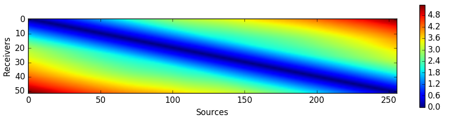
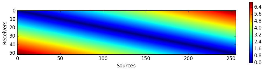
where is the model such that . For we use Neumann boundary conditions, since those lead to an effect of an automatic salt flooding, which is a popular way to treat salt bodies. We set the regularization parameter to be . We note that other choices of and regularization terms may definitely be suitable here, but are beyond the scope of this paper. Figure 7(c) shows the result model of the Gauss Newton minimization, and Figure 8 presents the initial and final data and data residuals. In particular, Figure 8(d) shows that the final residual mostly contains the added Gaussian noise. Figure 9 shows that the misfit was indeed reduced throughout the iterations, until the reduction stalls and the misfit reflect the noise level.


To demonstrate our algorithm in 3D, we use a 3D version of the same SEG/EAGE model, presented in Figure 10(a), using a grid that represents a volume of . We choose 144 equally distanced sources locations on the open surface, located every 23 pixels on the top surface, and receivers located on the top surface. We use the same parameters as in the 2D experiment (bound function, regularization, initial 3D model, added noise to the data, number of iterations etc.). Figure 10(b) shows the result of the inversion. Similarly to the 2D case, the top part of the model is recovered quite well, while a “salt flooding” effect is evident in the bottom part of the model. We performed the inversion using a machine with two Intel(R) Xeon(R) E5-2670 v3 processors with 128 GB of RAM. Using 24 cores, we applied the inversion in approximately 15 hours, and the highest memory footprint of the algorithm reached around 30GB.


7 Conclusions
In this paper we developed a Fast Marching algorithm for the factored eikonal equation, which in many cases yields a more accurate solution of the travel time than the original equation. Similarly to the original FM algorithm, our version solves the factored problem by exploiting the monotonicity of the solution along the characteristics. Our algorithm is capable of solving the problem using both first and second order schemes. The advantages of our algorithm are (1) its favorable guaranteed running time, and (2) the easily computed sensitivity matrices for solving the inverse (factored) eikonal equation.
8 Acknowledgement
The research leading to these results has received funding from the European Union’s - Seventh Framework Programme (FP7/2007-2013) under grant agreement no 623212 - MC Multiscale Inversion.
References
References
- [1] F. Aminzadeh, B. Jean, and T. Kunz, 3-D salt and overthrust models, Society of Exploration Geophysicists, 1997.
- [2] J. A. Bærentzen, On the implementation of fast marching methods for 3D lattices, Tech. Report IMM-TR-2001-13, Informatics and Mathematical Modelling, Technical University of Denmark, DTU, Richard Petersens Plads, Building 321, DK-2800 Kgs. Lyngby, 2001.
- [3] A. Benaichouche, M. Noble, and A. Gesret, First arrival traveltime tomography using the fast marching method and the adjoint state technique, in 77th EAGE Conference Proceedings., 2015.
- [4] J. Bezanzon, S. Karpinski, V. Shah, and A. Edelman, Julia: A fast dynamic language for technical computing, in Lang.NEXT, Apr. 2012.
- [5] M. G. Crandall and P.-L. Lions, Viscosity solutions of Hamilton-Jacobi equations, Transactions of the American Mathematical Society, 277 (1983), pp. 1–42.
- [6] S. Fomel, S. Luo, and H. Zhao, Fast sweeping method for the factored eikonal equation, Journal of Computational Physics, 228 (2009), pp. 6440–6455.
- [7] P. A. Gremaud and C. M. Kuster, Computational study of fast methods for the eikonal equation, SIAM journal on scientific computing, 27 (2006), pp. 1803–1816.
- [8] E. Haber, Computational Methods in Geophysical Electromagnetics, vol. 1, SIAM, 2014.
- [9] E. Haber and S. MacLachlan, A fast method for the solution of the Helmholtz equation, Journal of Computational Physics, 230 (2011), pp. 4403–4418.
- [10] C. Y. Kao, S. Osher, and J. Qian, Lax–friedrichs sweeping scheme for static Hamilton-Jacobi equations, Journal of Computational Physics, 196 (2004), pp. 367–391.
- [11] R. Kimmel and J. A. Sethian, Computing geodesic paths on manifolds, Proceedings of the National Academy of Sciences, 95 (1998), pp. 8431–8435.
- [12] S. Leung, J. Qian, and R. Burridge, Eulerian Gaussian beams for high-frequency wave propagation, Geophysics, 72 (2007), pp. SM61–SM76.
- [13] S. Leung, J. Qian, et al., An adjoint state method for three-dimensional transmission traveltime tomography using first-arrivals, Communications in Mathematical Sciences, 4 (2006), pp. 249–266.
- [14] S. Li, A. Vladimirsky, and S. Fomel, First-break traveltime tomography with the double-square-root eikonal equation, Geophysics, 78 (2013), pp. U89–U101.
- [15] S. Luo and J. Qian, Factored singularities and high-order lax–friedrichs sweeping schemes for point-source traveltimes and amplitudes, Journal of Computational Physics, 230 (2011), pp. 4742–4755.
- [16] , Fast sweeping methods for factored anisotropic eikonal equations: multiplicative and additive factors, Journal of Scientific Computing, 52 (2012), pp. 360–382.
- [17] S. Luo, J. Qian, and R. Burridge, Fast Huygens sweeping methods for Helmholtz equations in inhomogeneous media in the high frequency regime, Journal of Computational Physics, 270 (2014), pp. 378–401.
- [18] S. Luo, J. Qian, and R. Burridge, High-order factorization based high-order hybrid fast sweeping methods for point-source eikonal equations, SIAM Journal on Numerical Analysis, 52 (2014), pp. 23–44.
- [19] S. Luo, J. Qian, and H. Zhao, Higher-order schemes for 3d first-arrival traveltimes and amplitudes, Geophysics, 77 (2012), pp. T47–T56.
- [20] M. Noble, A. Gesret, and N. Belayouni, Accurate 3-d finite difference computation of traveltimes in strongly heterogeneous media, Geophysical Journal International, 199 (2014), pp. 1572–1585.
- [21] A. Pica et al., Fast and accurate finite-difference solutions of the 3d eikonal equation parametrized in celerity, 67th Ann. Internat. Mtg, Soc. of Expl. Geophys, (1997), pp. 1774–1777.
- [22] J. Qian and W. W. Symes, An adaptive finite-difference method for traveltimes and amplitudes, Geophysics, 67 (2002), pp. 167–176.
- [23] J. Qian, Y.-T. Zhang, and H.-K. Zhao, A fast sweeping method for static convex Hamilton-Jacobi equations, Journal of Scientific Computing, 31 (2007), pp. 237–271.
- [24] N. Rawlinson and M. Sambridge, Wave front evolution in strongly heterogeneous layered media using the fast marching method, Geophysical Journal International, 156 (2004), pp. 631–647.
- [25] E. Rouy and A. Tourin, A viscosity solutions approach to shape-from-shading, SIAM Journal on Numerical Analysis, 29 (1992), pp. 867–884.
- [26] L. I. Rudin, S. Osher, and E. Fatemi, Nonlinear total variation based noise removal algorithms, Physica D: Nonlinear Phenomena, 60 (1992), pp. 259–268.
- [27] L. Ruthotto, E. Treister, and E. Haber, jInv – a flexible Julia package for PDE parameter estimation, Submitted, (2016).
- [28] C. Saragiotis, T. Alkhalifah, and S. Fomel, Automatic traveltime picking using instantaneous traveltime, Geophysics, 78 (2013), pp. T53–T58.
- [29] A. Sei, W. W. Symes, et al., Gradient calculation of the traveltime cost function without ray tracing, in 65th Ann. Internat. Mtg., Soc. Expl. Geophys., Expanded Abstracts, 1994, pp. 1351–1354.
- [30] J. A. Sethian, A fast marching level set method for monotonically advancing fronts, Proceedings of the National Academy of Sciences, 93 (1996), pp. 1591–1595.
- [31] , Fast marching methods, SIAM review, 41 (1999), pp. 199–235.
- [32] E. Somersalo and J. Kaipio, Statistical and computational inverse problems, Applied Mathematical Sciences, 160 (2004).
- [33] A. Spira and R. Kimmel, An efficient solution to the eikonal equation on parametric manifolds, Interfaces and Free Boundaries, 6 (2004), pp. 315–328.
- [34] C. Taillandier, M. Noble, H. Chauris, and H. Calandra, First-arrival traveltime tomography based on the adjoint-state method, Geophysics, 74 (2009), pp. WCB1–WCB10.
- [35] Y.-H. R. Tsai, L.-T. Cheng, S. Osher, and H.-K. Zhao, Fast sweeping algorithms for a class of Hamilton-Jacobi equations, SIAM journal on numerical analysis, 41 (2003), pp. 673–694.
- [36] J. N. Tsitsiklis, Efficient algorithms for globally optimal trajectories, Automatic Control, IEEE Transactions on, 40 (1995), pp. 1528–1538.
- [37] C. R. Vogel, Computational methods for inverse problems, vol. 23, SIAM, Philadelphia, 2002.
- [38] H. Zhao, A fast sweeping method for eikonal equations, Mathematics of computation, 74 (2005), pp. 603–627.