Many-body quantum interference on hypercubes

The $d$-dimensional hypercube consists of $n=2^{d}$ modes, each connected to $d$ neighbours as illustrated in Figure 1.

Note that this system may be seen as a generalisation of a $2$-site graph in $d$ dimensions. Let $\hat{\mathcal{H}}_{i,j}/\hbar=\kappa$ be the transition rate for neighbouring sites $i$ and $j$. For an evolution time $t=\pi/(4\kappa)$, the unitary transformation matrix reads

It contains all single-particle transformation amplitudes and is the basis for calculating many-particle amplitudes according to (3)-(5). Due to the tensor power in (3.1), the unitary clearly exhibits stepwise symmetries. Pertaining to equation (2), an explicit expression for the element $\hat{U}_{j,k}$ is required to make the importance of symmetries apparent. To obtain such an expression, sign-bookkeeping instruments are introduced: We define segmentation parameters $p\in\{2,4,8,\dots,n\}$ and their corresponding Rademacher functions [34]

where the Gaussian brackets $\left\lfloor\alpha/\beta\right\rfloor$ evaluate the quotient of the Euclidean division $\alpha/\beta$. The Rademacher functions, exemplified for $d=3$ in the first three rows of table 1, assign the value $1$ ($-1$) to modes $j\in\{1,\dots,n\}$ as determined by the segmentation value $p$ in a symmetric and stepwise fashion, such that all modes are clearly grouped into two subsets of the same size.

Returning to unitary (3.1), each element differs by a phase shift, equalling an integer multiple of $\pi/2$. The actual phase of element $\hat{U}_{i,j}$ can be calculated by means of the segmentations $p$, accounting for the accumulation of phases in the $i$-th row and $j$-th column. Thus, the elements of the unitary can be written as

as shown in A. The simple phase relation in this expression is of advantage when evaluating interference contributions for the calculation of transition probabilities in (2).

Note that the unitary (3.1) is equivalent to the one considered in [22] except for local phase operations. Consequently, suppression laws have also been discovered in Sylvester interferometers for specific initial states with particle numbers in powers of two. As we show in the following, however, by making use of the HC symmetries, one can prove suppression laws for a much larger class of particle configurations.

We consider the self-inverse symmetry operations

where $1\!\!1$ denotes the $2\times 2$ identity matrix and $\sigma_{x}$ the $2\times 2$ Pauli spin-x-operator. These symmetry operators are mutually commuting and act on mode occupation lists as $p/2$ transpositions of all $p$ segments, according to

which can be interpreted as a reflection in dimension $\log_{2}(p)$. Moreover, a consecutive action of symmetry operations with different $p$ values, where each operator acts at most once, is denoted by

with $\bi{p}=(p_{1},p_{2},\dots)$ and $\left|\left|\bi{p}\right|\right|$ denoting the number of elements in $\bi{p}$. Thus, the total number of possible symmetry operations for the $d$ dimensional HC corresponds to the number of subsets of $(2,4,\dots,2^{n})$, omitting the empty list. These $2^{d}-1$ self-inverse symmetries are key to the classification of the arising many-particle interferences. Figure 2 demonstrates the case of a three dimensional HC, where all self-inverse operations are assigned to familiar symmetries. For compositions of symmetry-operators, it is convenient to introduce Walsh functions [35]

which assign $1$ $(-1)$ to all modes as governed by the symmetry set $\bi{p}$, thereby partitioning all modes into two complementary subsets $\mathcal{P}(\bi{p})=\{j\in\{1,\dots,n\}\ |\ \mathcal{A}(j,\bi{p})=-1\}$ and $\bar{\mathcal{P}}(\bi{p})=\{j\in\{1,\dots,n\}\ |\ \mathcal{A}(j,\bi{p})=1\}$. For the sake of completeness, the lower rows in table 1 list the partitionings for any composite set $\bi{p}$ on the three dimensional HC.

For initial states, being invariant under the symmetry operation

the symmetry of the unitary is in some way preserved in matrix $M$. Note that an initial state can be invariant under various symmetries which may be related to each other. In this regard, we denote the number of independent symmetries of an initial state by $\eta$, being the minimal number of symmetry operations with which one can compose all symmetry operations the initial state is invariant under¹¹ 1 Recalling that the symmetry operators $\mathcal{S}(\bi{p})$ are self-inverse and mutually commute, we define the set $\Gamma=\{\bi{p}\ |\ \mathcal{S}(\bi{p})\ \bi{r}=\bi{r}\}$ and all possible sets $\Lambda_{k}\subseteq\Gamma\ :\ \forall\bi{p}\in\Gamma\ \exists\ T\subseteq\Lambda_{k}\ :\ \prod_{\bi{p}_{j}\in T}\mathcal{S}(\bi{p}_{j})=\mathcal{S}(\bi{p})$, which generate all symmetry operations the initial state is invariant under. Then, the number of independent symmetries of $\bi{r}$ is given by $\eta=\min\{\left|\Lambda_{1}\right|,\left|\Lambda_{2}\right|,\dots\}$. For example, if $\bi{r}$ is invariant under $\mathcal{S}(2)$, $\mathcal{S}(8)$ and $\mathcal{S}((2,8))$, then $\Lambda_{1}=\{2,8,(2,8)\}$, $\Lambda_{2}=\{2,8\}$, $\Lambda_{3}=\{2,(2,8)\}$, $\Lambda_{4}=\{8,(2,8)\}$ and accordingly $\eta=2$. . In order to satisfy condition (15), particles must be arranged in a configuration which is invariant under all independent symmetries. Therefore, the particle number is restricted to $N=z\cdot 2^{\eta}$ with $z\in\mathbb{N}$.

Under these conditions, the underlying symmetry can lead to a vanishing transition probability for certain final states. This arises from the $N$-particle transition amplitudes of (2) summing up in pairs of permutations, which cancel out due to their opposite phases. The partitioning of all $n$ modes according to the Walsh functions in (14) then allows the formulation of suppression laws, that predict which final states are suppressed:

Bosons: For an initial state $\bi{r}$ of $N$ indistinguishable bosons, which is invariant under the symmetry operation $\mathcal{S}(\bi{p})$, such that $N$ must be even, all final states $\bi{s}$ with an odd number of particles in the subset of modes $k$ for which $\mathcal{A}(k,\bi{p})=-1$, are suppressed, i.e.,

Fermions: For an initial state $\bi{r}$ of $N$ indistinguishable fermions, which is invariant under the symmetry operation $\mathcal{S}(\bi{p})$, such that $N$ must be even, all final states $\bi{s}$, that do not have exactly $N/2$ particles in the subset of modes $k$ for which $\mathcal{A}(k,\bi{p})=-1$, are suppressed, i.e.,

The proofs of these suppression laws are given in B. The direct connection of the involved symmetries to the condition for total destructive interference is immediately apparent by comparing the symmetry operation (13) with the partitioning (14). These symmetries simplify the underlying complexity of many-particle evolutions in a demonstrative way (see section 3.5 for an explicit example). Even if no statement about probabilities of non-vanishing events is made by the suppression laws (16a) and (16b) themselves, they are obtained purely analytically, thereby permitting a prediction which final states must be suppressed with little computational overhead.

A deeper comparison of the suppression laws for bosons and fermions reveals an interesting connection: First of all, fermions feature a much more general condition for suppression as compared to bosons, such that the set of allowed configurations is more restricted for the former. Whether the suppressed boson states are also forbidden for fermions depends on the parity of $N/2$: For particle numbers satisfying $\mathrm{\ mod}[N,4]=0$ the two suppression conditions coincide, that is, states with an odd number of particles occupying the relevant set of modes are suppressed for both types of particles. However, for $\mathrm{\ mod}[N,4]=2$, the conditions are complementary to each other. A similar effect was discovered in the studies of the discrete Fourier transform in [20], where the particle number also determines whether or not the suppression law for many-fermion states resembles the one for bosons.

In order to highlight the extent of many-body destructive interference on the considered graphs, the suppression ratios $\mathcal{N}_{\mathrm{supp}}/\mathcal{N}_{\mathrm{all}}$ for the derived suppression laws (16a) and (16b) are discussed in the following. Here $\mathcal{N}_{\mathrm{all}}$ denotes the total number of final states and $\mathcal{N}_{\mathrm{supp}}$ the predicted number of suppressed states.

According to the suppression law (16a), for bosonic initial states, which are invariant under a single independent symmetry operation ($\eta=1$), one expects the suppression of about half of all possible final states. To respect common suppressed states of different independent symmetries, the intersection of their respective subsets $\mathcal{P}(\bi{p})$ and $\mathcal{P}(\bi{p}^{\prime})$ has to be considered. From the definition of the Walsh functions in (14), one finds $\sum_{j=1}^{n}\mathcal{A}(j,\bi{p})\mathcal{A}(j,\bi{p}^{\prime})=0$ for $\bi{p}\neq\bi{p}^{\prime}$ (see for example table 1). Recalling that $\mathcal{P}(\bi{p})$ and $\bar{\mathcal{P}}(\bi{p})$ are complementary sets of equal size, this implies that subsets corresponding to different symmetry operations share half of their elements, i.e. $|\mathcal{P}(\bi{p})\cap\mathcal{P}(\bi{p}^{\prime})|=|\mathcal{P}(\bi{p})|/2=n/4$. Thus, two different independent symmetries have about half of all suppressed final states in common. It follows, that the suppression ratio for those bosonic initial states can be approximated for large $n$ by

In the case of fermions, for each independent symmetry, the suppression law (16b) forces all particles to distribute equally among the two complementary subsets, regardless to the occupation within each individual subset. Furthermore, subsets corresponding to different symmetries share one half of their elements. Thus, for $\eta$ independent symmetries the total number of subsets, among which particles are forced to distribute equally, is given by $2^{\eta}$. Accordingly, the number of states, which are not covered by the suppression law (16b), is given by ${n/2^{\eta}\choose N/2^{\eta}}^{2^{\eta}}$. Because Pauli’s principle excludes modes with multiple occupation, the total number of final states reads $\mathcal{N}_{\mathrm{all}}={n\choose N}$, resulting in

with the approximation valid for $n\gg N$. Due to symmetry reasons, fermionic initial states with particle numbers satisfying $\mathrm{\ mod}[N,4]=2$ can only be invariant under at most one independent symmetry operation. However, states with particle numbers $N=2^{\eta}$ can satisfy up to $\eta$ independent symmetry operations leading to a suppression ratio $\mathcal{N}^{\mathrm{F}}_{\mathrm{supp}}/\mathcal{N}^{\mathrm{F}}_{\mathrm{all}}\approx 1-N!/N^{N}$. For comparison, Figure 3 illustrates the suppression ratios for bosons and fermions in the limit $n\gg N$. It is evident how, for a fixed number of independent symmetries, more fermionic states are suppressed than for bosons and that fermionic suppression gets increasingly restrictive for growing particle numbers.

To exemplify the above suppression law, a scattering scenario of $N=8$ bosons on the HC for $d=3$ dimensions is considered. In total there are ${N+n-1\choose N}=6435$ possibilities to distribute the particles over the $n=8$ modes, whereof three initial states are chosen for discussion. For these states, Figure 4 shows the transition probabilities for all possible final states $\bi{s}$.

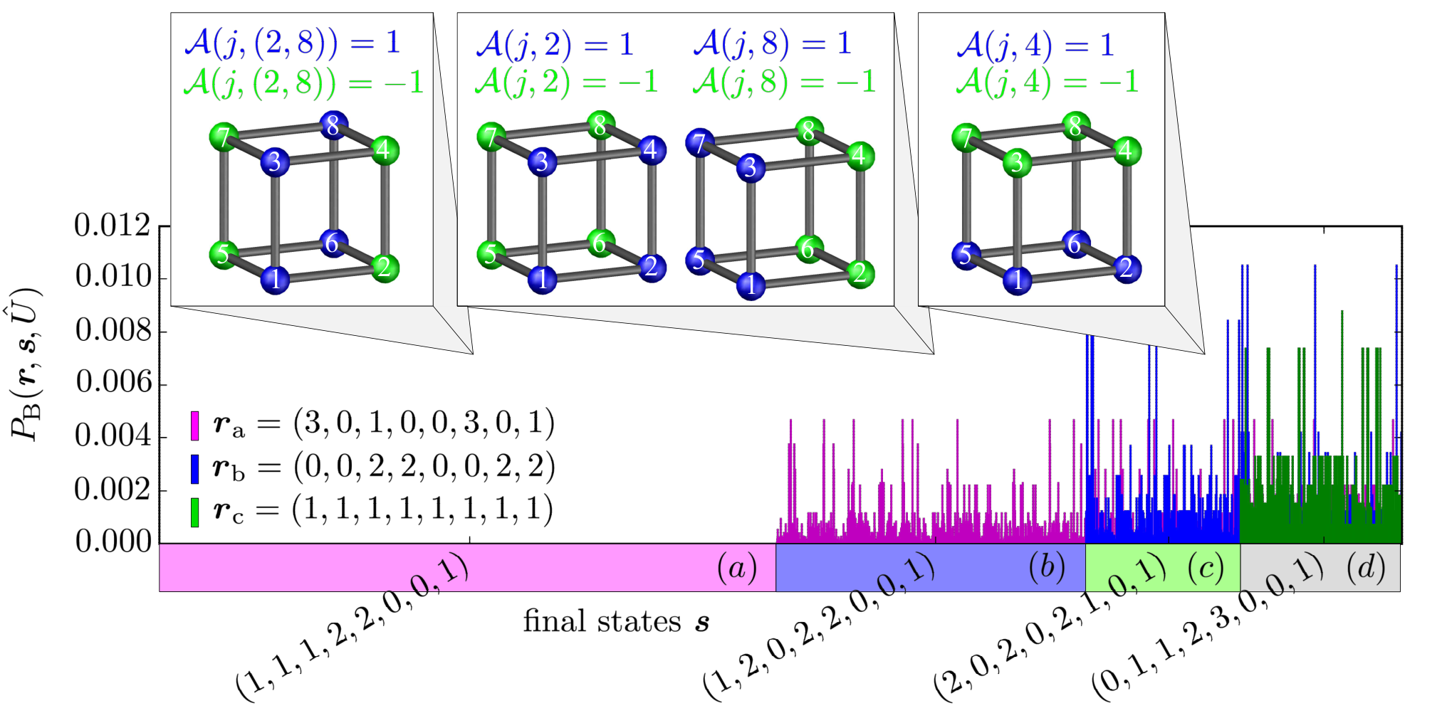
The initial state $\bi{r}_{\mathrm{a}}=(3,0,1,0,0,3,0,1)$ is only invariant under the operation $\mathcal{S}((2,8))$, causing the suppression of all final states with an odd number of bosons in the subset of modes $k$ for which $\mathcal{A}(k,(2,8))=-1$. These states are grouped in set $(a)$ of Figure 4, where the corresponding partitioning is visualized in the first inset. One representative of those is the final state $\bi{s}=(1,1,1,2,2,0,0,1)$ containing three (five) bosons in modes $k$ for which $\mathcal{A}(k,(2,8))=1$ ($-1$).

The second initial state under consideration, $\bi{r}_{\mathrm{b}}=(0,0,2,2,0,0,2,2)$, is invariant under the operations $\mathcal{S}(2)$ and $\mathcal{S}(8)$ and accordingly also under $\mathcal{S}((2,8))$. Thus, in addition to the suppressed final states for $\bi{r}_{\mathrm{a}}$, states with an odd number of bosons in the subset of modes $k$ for which $\mathcal{A}(k,2)=-1$ and an odd number in the subset of modes with $\mathcal{A}(k,8)=-1$ must also be suppressed. This is shown in set $(b)$ in Figure 4. One representative of this set is the final state $\bi{s}=(1,2,0,2,2,0,0,1)$, exhibiting five (three) bosons in modes $k$ for which $\mathcal{A}(k,2)=1$ ($-1$) and three (five) bosons in modes $k$ for which $\mathcal{A}(k,8)=1$ ($-1$). For clarity, the second inset illustrates the partitionings for $p=2$ and $p=8$.

In this scattering scenario, the initial states with the largest number of invariant symmetry operations is given by $\bi{r}_{\mathrm{c}}=(1,1,1,1,1,1,1,1)$. Therefore, states with an odd number of bosons in the subset of modes $k$ for which $\mathcal{A}(k,4)=-1$ must also be suppressed in addition to all states already suppressed for $\bi{r}_{\mathrm{b}}$. In Figure 4, these states are grouped in set $(c)$, excluding those, already contained in set $(a)$ and $(b)$. The corresponding inset shows the partitioning for $p=4$. As a representative, the state $\bi{s}=(2,0,2,0,2,1,0,1)$ is chosen, containing five (three) bosons in modes $k$ for which $\mathcal{A}(k,4)=1$ ($-1$). All remaining final states that are not covered by the suppression law for any $\bi{p}$, like $\bi{s}=(0,1,1,2,3,0,0,1)$, are grouped in set $(d)$.

Here it becomes apparent that the symmetry of many-body initial states determines a well structured appearance of total destructive interference on HC graphs. It also highlights the interdependence of different symmetry operations. For example, the initial state $\bi{r}_{\mathrm{b}}$ is invariant under two independent symmetry operations, namely $\mathcal{S}(2)$ and $\mathcal{S}(8)$. From this follows that the state must be invariant under a composition of both operators as well. Thus final states, which are suppressed for $\bi{r}_{\mathrm{a}}$ (invariant under $\mathcal{S}((2,8))$) and covered by the suppression law, must also be suppressed for $\bi{r}_{\mathrm{b}}$. However, since $\bi{r}_{\mathrm{a}}$ is only invariant under $\mathcal{S}((2,8))$, states which are suppressed for $\bi{r}_{\mathrm{b}}$ are not necessarily suppressed for $\bi{r}_{\mathrm{a}}$.

Figure 4 also demonstrates the approximated suppression ratio (16q) in dependence on the number of independent symmetries an initial state is invariant under. Since $\bi{r}_{\mathrm{a}}$ is only invariant under $\mathcal{S}((2,8))$, half of all final states are expected to be suppressed, as apparent by the size of set $(a)$ in Figure 4. For each further independent symmetry, one clearly sees the additional suppression of half of the remaining final states from the size reduction of the other sets.

Now, in order to generalize the derived suppression laws, $d$-dimensional HC graphs are considered where each vertex consists of the same but arbitrary subgraph. Each subgraph then contains $m$ modes. Besides the coupling within each subgraph, each mode must be equally coupled to its $d$ identical counterparts in the predetermined HC ordering. This generalizes the model considerably since the HC-vertices are allowed to have diverse internal degrees of freedom. Such scenarios can be described by means of a $m\times m$ subunitary $\hat{A}$, where the overall unitary

consists of $2^{2d}$ subunitaries. In order to retain the HC symmetries for segmentations $p\in\{2,4,8,\dots,2^{d}\}$, the symmetry operations (11) are generalised to

by replacing the Pauli spin-x-operator with the exchange-operator $\Sigma_{x}$ of dimension $2m\times 2m$, reading

Here $\hat{0}_{m\times m}$ denotes the $m\times m$ null matrix and $1\!\!1_{m\times m}$ the $m\times m$ identity matrix. These modifications are sufficient in order to make the symmetry suppression laws (16a) and (16b) applicable to any unitary given by (4.1). The detailed proof is given in C.

Remarkably, for symmetry reasons, the suppression laws for these generalized graphs require the symmetric occupation of all modes for initial states. However, for final states, only the total number of particles within the subgraphs is relevant. Thus, the prediction whether or not a final state must be suppressed, is independent on its occupation within the subgraph, as will be further discussed in the following.

In order to illustrate the generalization, bosonic state transformations in one-dimensional HC graphs are considered. Figure 5 illustrates the mode coupling for identical subgraphs. Here, related modes of different subgraphs are equally connected by the transition rate $\kappa$, whereas transition rates within subgraphs are arbitrary but identical.

As apparent by the unitary (4.1) and by comparing Figure 5$(a)$ and 5$(b)$, for the suppression law, generalized HC graphs of the same dimension are closely related, regardless of structure and size of the subgraphs. Thus, we restrict the discussion of the examples shown in Figure 5 to the generalized graph with triangular subgraph.

Considering the mode labelling as shown in Figure 5$(a)$, the four-particle initial state $\bi{r}_{\mathrm{a}}=(2,0,0,2,0,0)$ is invariant under symmetry operation (16v) for $p=2$. Then, for an evolution time $t=\pi/(4\kappa)$, the generalized suppression law predicts, that all final states with an odd number of particles on any subgraph must be suppressed. Formally, this can be seen by considering definition (14), which gives $\mathcal{A}(j,2)=1$ for $j\in\{1,\dots,m\}$ and $\mathcal{A}(j,2)=-1$ for $j\in\{m+1,\dots,2m\}$ with $m=3$ in the discussed example. Since each mode of a particular subgraph belongs to the same subset (i.e. their partitioning value $\mathcal{A}(j,p)$ is equal), the condition for suppression appears independently of the particle occupation within the subgraphs. Thus, for example the final states $\bi{s}=(3,0,0,0,1,0)$ and $\bi{s}=(1,1,1,0,1,0)$ must be suppressed for $\bi{r}_{\mathrm{a}}$. However, in agreement with the formal suppression law, they appear with a non-vanishing probability for the initial state $\bi{r}_{\mathrm{b}}=(2,0,0,1,1,0)$. This highlights that the condition for suppression strongly depends on the initial particle occupation within the subgraphs as determined by the invariance under the symmetry operations (16v), which $\bi{r}_{\mathrm{b}}$ does not fulfil.

References

- [1] A. M. Childs et al., Exponential Algorithmic Speedup by a Quantum Walk, Proceedings of the Thirty-fifth Annual ACM Symposium on Theory of Computing, 59–68, ACM, (2003).
- [2] S. Bose, Quantum Communication through an Unmodulated Spin Chain, Phys. Rev. Lett. 91, 207901 (2003).
- [3] N. Y. Yao et al., Scalable architecture for a room temperature solid-state quantum information processor, Nat. Commun. 3, 800 (2012).
- [4] S. Sahling et al., Experimental realization of long-distance entanglement between spins in antiferromagnetic quantum spin chains, Nat. Phys. 11, 255–260 (2015).
- [5] G. S. Engel et al., Evidence for wavelike energy transfer through quantum coherence in photosynthetic systems, Nature 446, 782–786 (2007).
- [6] N. Lambert et al., Quantum biology, Nat. Phys. 9, 10–18 (2013).
- [7] C. K. Hong, Z. Y. Ou and L. Mandel, Measurement of subpicosecond time intervals between two photons by interference, Phys. Rev. Lett. 59, 2044–2046 (1987).
- [8] R. C. Liu et al., Quantum interference in electron collision, Nature 391, 263–265 (1998).
- [9] R. Loudon, Fermion and boson beam-splitter statistics, Phys. Rev. A 58, 4904–4909 (1998).
- [10] A. Peruzzo et al., Quantum Walks of Correlated Photons, Science 329, 1500–1503 (2010).
- [11] M. C. Tichy, Interference of identical particles from entanglement to boson-sampling, J. Phys. B 47, 103001 (2014).
- [12] K. Mattle et al., Non-Classical Statistics at Multiport Beam Splitters, Appl. Phys. B 60, S111 (1995).
- [13] A. M. Kaufman et al., Two-particle quantum interference in tunnel-coupled optical tweezers, Science 345, 306–309 (2014).
- [14] J. Carolan et al., On the experimental verification of quantum complexity in linear optics, Nat. Photon. 8, 621–626 (2014).
- [15] K. Poulios et al., Quantum Walks of Correlated Photon Pairs in Two-Dimensional Waveguide Arrays, Phys. Rev. Lett. 112, 143604 (2014).
- [16] A. Crespi et al., Particle Statistics Affects Quantum Decay and Fano Interference, Phys. Rev. Lett. 114, 090201 (2015).
- [17] N. Spagnolo et al., Three-photon bosonic coalescence in an integrated tritter, Nat. Commun. 4, 1606 (2013).
- [18] M. Christandl et al., Perfect State Transfer in Quantum Spin Networks, Phys. Rev. Lett. 92, 187902 (2004).
- [19] A. Kay, Perfect state transfer: Beyond nearest-neighbor couplings, Phys. Rev. A 73, 032306 (2006).
- [20] M. C. Tichy et al., Many-particle interference beyond many-boson and many-fermion statistics, New J. Phys. 14, 093015 (2012).
- [21] A. Crespi et al., Suppression law of quantum states in a 3D photonic fast Fourier transform chip, Nat. Commun. 7, (2016).
- [22] A. Crespi, Suppression laws for multiparticle interference in Sylvester interferometers, Phys. Rev. A 91, 013811 (2015).
- [23] C. Dittel et al., Efficient Certification of Boson Sampling in Waveguide Lattices with parity-like Symmetry, 2015 European Conference on Lasers and Electro-Optics - European Quantum Electronics Conference, JSV_3_5, Optical Society of America, (2015).
- [24] S. Weimann et al., Implementation of quantum and classical discrete fractional Fourier transforms, Nat. Commun. 7, (2016).
- [25] T. D. Mackay et al., Quantum walks in higher dimensions, J. Phys. A 35, 2745 (2002).
- [26] C. Moore and A. Russell, Quantum Walks on the Hypercube, Randomization and Approximation Techniques in Computer Science, 164–178, Springer Berlin Heidelberg, (2002).
- [27] J. Kempe, Discrete Quantum Walks Hit Exponentially Faster, Probab. Theory Related Fields 133, 215–235 (2005).
- [28] G. Alagic and A. Russell, Decoherence in quantum walks on the hypercube, Phys. Rev. A 72, 062304 (2005).
- [29] H. Krovi and T. A. Brun, Hitting time for quantum walks on the hypercube, Phys. Rev. A 73, 032341 (2006).
- [30] A. Makmal et al., Quantum walks on embedded hypercubes, Phys. Rev. A 90, 022314 (2014).
- [31] A. Makmal et al., Quantum walks on embedded hypercubes: Nonsymmetric and nonlocal cases, Phys. Rev. A 93, 022322 (2016).
- [32] K. Mayer et al., Counting statistics of many-particle quantum walks, Phys. Rev. A 83, 062307 (2011).
- [33] W. Pauli, Exclusion Principle and Quantum Mechanics, Nobel Lectures, Physics 1942-1962, Elsevier Publishing Company, Amsterdam (1964).
- [34] H. Rademacher, Einige Sätze über Reihen von allgemeinen Orthogonalfunktionen, Math. Annal. 87, 112–138 (1922).
- [35] J. L. Walsh, A Closed Set of Normal Orthogonal Functions, Am. J. Math. 45, 5-24 (1923).
- [36] R. A. Campos, B. E. A. Saleh and M. C. Teich, Quantum-mechanical lossless beam splitter: SU(2) symmetry and photon statistics, Phys. Rev. A 40, 1371–1384 (1989).
- [37] Z. Y. Ou, J.-K. Rhee and L. J. Wang, Observation of Four-Photon Interference with a Beam Splitter by Pulsed Parametric Down-Conversion, Phys. Rev. Lett. 83, 959–962 (1999).
- [38] S. Mostarda et al., Structure-dynamics relationship in coherent transport through disordered systems, Nat.Commun. 4, 2296– (2013).
- [39] M. Walschaers et al., Optimally Designed Quantum Transport across Disordered Networks, Phys. Rev. Lett. 111, 180601 (2013).
- [40] S. Aaronson and A. Arkhipov, The Computational Complexity of Linear Optics, Proceedings of the Forty-third Annual ACM Symposium on Theory of Computing, 333–342, ACM, (2011).
- [41] N. Spagnolo et al., Experimental validation of photonic boson sampling, Nature Photon. 8, 615–620 (2014).
- [42] M. C. Tichy et al., Stringent and Efficient Assessment of Boson-Sampling Devices, Phys. Rev. Lett. 113, 020502 (2014).
- [43] M. Walschaers et al., Statistical benchmark for Boson Sampling, New J.Phys. 18, 032001 (2016).
- [44] V. S. Shchesnovich, Partial indistinguishability theory for multiphoton experiments in multiport devices, Phys. Rev. A 91, 013844 (2015).
- [45] M. C. Tichy, Sampling of partially distinguishable bosons and the relation to the multidimensional permanent, Phys. Rev. A 91, 022316 (2015).
- [46] M. Tillmann et al., Generalized Multiphoton Quantum Interference, Phys. Rev. X 5, 041015 (2015).
- [47] J. L. O’Brien, Optical Quantum Computing, Science 318, 1567–1570 (2007).
- [48] L. Daqing et al., Dimension of spatially embedded networks, Nat. Phys. 7, 481–484 (2011).
- [49] D. Jukić and H. Buljan, Four-dimensional photonic lattices and discrete tesseract solitons, Phys. Rev. A 87, 013814 (2013).
- [50] O. Boada et al., Quantum Simulation of an Extra Dimension, Phys. Rev. Lett. 108, 133001 (2012).
- [51] M. Mancini et al., Observation of chiral edge states with neutral fermions in synthetic Hall ribbons, Science 349, 1510–1513 (2015).
- [52] B. K. Stuhl et al., Visualizing edge states with an atomic Bose gas in the quantum Hall regime, Science 349, 1514–1518 (2015).
- [53] M. Schmidt et al., Optomechanical creation of magnetic fields for photons on a lattice, Optica 2, 635–641 (2015).
- [54] T. Ozawa et al., Synthetic dimensions in integrated photonics: From optical isolation to 4D quantum Hall physics, ArXiv e-prints 1510.03910, (2015).
- [55] H. Defienne et al., Two-photon quantum walk in a multimode fiber, Sci. Adv. 2, (2016).
- [56] M. Reck et al., Experimental realization of any discrete unitary operator, Phys. Rev. Lett. 73, 58–61 (1994).
- [57] J. Carolan et al., Universal linear optics, Science 349, 711–716 (2015).
- [58] J. Mower et al., High-fidelity quantum state evolution in imperfect photonic integrated circuits, Phys. Rev. A 92, 032322 (2015).
- [59] J. C. F. Matthews et al., Observing fermionic statistics with photons in arbitrary processes, Sci. Rep. 3, 1539– (2013).