On frequency and time domain models of traveling wave tubes
Abstract
We discuss the envelope modulation assumption of frequency-domain models of traveling wave tubes (TWTs)
and test its consistency with the Maxwell equations.
We compare the predictions of usual frequency-domain models
with those of a new time domain model of the TWT.
Keywords :
traveling wave tube, wave-particle interaction, time-domain simulation,
Gel’fand -transform, envelope modulation
PACS numbers: 84.40.Fe (microwave tubes)
52.35.Fp (Plasma: electrostatic waves and oscillations)
52.40.Mj (particle beam interaction in plasmas)
52.20.Dq (particle orbits)
I Introduction
Two approaches are usually applied in describing the dynamics in a traveling wave tube (TWT) : (i) the time domain approach makes no assumption on the TWT working frequency, nor even on the shape of the signal wave, while (ii) the frequency domain approach implies that all variables of interest depend on time like . So-called multi-frequency models can accommodate several frequencies, provided they are multiples of a fundamental frequency. This hampers the prediction of non-harmonic instabilities, as may result from nonlinearities or defects.
Current simulations for TWT design rely mainly on frequency domain models because of their fast numerical execution. However, the current need for higher power and gain brings these models to the limits of their reliability. Therefore, we develop a family of time domain models [1, 2, 3, 5] inspired by [8, 13], in order to provide more compact, accurate and complete descriptions of such regimes. This paper compares this time-domain approach and frequency models, as well as the foundations of the latter.
In section II, we revisit a central assumption of industrial frequency models [4, 9, 10, 14] and discuss its consistency with Maxwell equations when applied to three-dimensional geometry. Then, we rederive the basic equation for the modulation amplitude in frequency models. In section III, we compare frequency-domain models to assess the importance of the selection of modes which must be made in order to run the model. In section IV, we recall the principles of our discrete model, which we compare to frequency-domain models in section V to assess their mutual consistency.
II Consistency of frequency models
Frequency domain models used in the industry share a common representation of the electromagnetic field interacting with the electron beam. The “hot” field at frequency is simply the sum of “beamless” modes modulated by an envelope factor function of the axial position only. One [14] or several [4, 10] modes can be used in this expansion. The term “mode” refers to the different propagating modes existing in the delay line at the considered frequency , each mode having a real propagating constant as shown in Fig. 1. Consequently, we write in harmonic form
| (1) | |||||
| (2) |
The envelope factors are the ’s, and is the longitudinal coordinate along the tube axis, with unit vector . In this paper, we call such models Cold Wave Amplification Models (CoWAMs). The real electric field is when only one frequency is considered. The case of several frequencies, in particular harmonics, can be treated by summing the expansions at each considered frequency. Hereafter, only one frequency is considered.
By definition, the cold fields and solve the homogeneous Maxwell equations in harmonic form, viz. the Helmholtz equation,
| (3) | |||||
| (4) |
with appropriate boundary conditions.

In presence of a beam, the physical fields and must satisfy the full Maxwell equations, in particular Maxwell-Faraday for . The electric field then reads
| (5) |
where the space-charge field is a gradient. Then the curl of the full field is only the curl of the circuit field (1),
| (6) | |||||
where the second equality follows from a vector analysis identity and the third equality results from (3). Finally, recalling (2) yields
| (7) |
The Maxwell-Faraday equation states that the left-hand side must vanish. Therefore, the envelope form (1)-(2) is consistent with the Maxwell equations only if the right hand side vanishes. If the electric field of each mode is purely longitudinal, this condition is met automatically.
However, generically the electric field is not purely longitudinal through the whole cross section of the structure. Otherwise the Poynting vector would be purely transverse and the considered mode would carry no power. This precludes the possibility to use a single mode in the expansion (1). Indeed, the only possibility to satisfy the Maxwell-Faraday equation with a single cold mode is that , i.e. that no amplification occurs. In practice, is slowly varying, so that remains low enough for a good approximation.
The expansion on a single mode violates the Maxwell equations, so the question is now to determine whether they can be satisfied by an expansion on several modes.
To this end, consider the Maxwell-Ampère equation
| (8) |
and recall that . Again, substituting (1)-(2)-(5) and using the same vector identity yields
| (9) |
Denote by the Fourier component of . Multiplying (9) with and using a vector identity obtains
| (10) |
Similarly, dot-multiplying (7) with and using a vector identity yields
| (11) |
at every point .
Subtracting (11) from (10) and integrating over a transverse, planar section yields
| (12) | |||||
For a periodic structure (as considered in mvtrad [14], christine [4] and bwis [10]), the integral in the left hand side vanishes for , thanks to the mode orthogonality relation [6]
| (13) |
where is the absolute value of the (longitudinal) electromagnetic power flow in mode (incorporating the normalization of the eigenfields and ) and according to the direction of the power flow. Equation (12) so reduces to
| (14) |
These are necessary, but not sufficient, conditions to satisfy the Maxwell equations. Equations (14) completely determine the amplitude of the wave inside the TWT, along with the dynamics of the electrons. At this point, we can make an important remark on which modes will be amplified or not. At the start of the amplification process, all modes have small amplitude and the TWT operates in the linear regime. We know that in this case the beam is carrying space charge waves [11]. These waves have their own wave number which is given by the beam velocity in a first order approximation, . Therefore, only modes with close to will grow significantly in equation (14), because otherwise the right hand side is the integral of an oscillating function. This will be illustrated in the next section with a numerical example.
Now, we compare the relative importance of these waves in term of power by calculating the total power flow from the Poynting vector. The same orthogonality theorem gives (with c.c. denoting complex conjugate)
| (15) |
i.e., the total power results from the power carried by each individual mode. Introducing the mode amplitude [11], the power of each mode is simply and equation (15) becomes
| (16) |
where is the coupling impedance of mode at the working frequency and is the electric field of that mode divided by its amplitude. With this final form of the interaction equation, we can see that modes with large coupling impedance will rapidly dominate over modes of low coupling impedance as we move toward the TWT output.
To conclude this part, we are left with a contradiction. We have just seen that only the modes synchronized with the beam can grow, as confirmed by dedicated experiments [7]. In the usual situation of a practical TWT, only one mode satisfies this synchronization condition. Therefore, this mode alone rapidly dominates in the amplification process. But we have also seen that the Maxwell equations cannot be satisfied with a single mode. It follows that the envelope model (CoWAM) can only approximate the physics. How accurate this approximation is remains difficult to assess. One motivation to develop the discrete model, beside its time domain capabilities, is to lift these theoretical approximations. Based on our experience however, we expect that the approximation is minor, at least inside common ranges of parameters used for practical devices. This fact will also be illustrated hereafter with a numerical example.
III Relevance of backward wave in CoWAM
In this numerical example, we assess the relative importance of the forward and backward modes for a standard helix tube. Such a tube comprises attenuating sections, where the fields are partly absorbed ; these attenuating sections are modeled in CoWAMs on adding a loss term in (14) to give
| (17) |
where the spatial loss rate is a function of position accounting for propagation losses and localized attenuator. The purpose of the present calculation is to compare the relative power of the different modes radiated by a given modulated electron beam. Consequently, the current density is an input generated from a preliminary run of mvtrad. The same modulated current density is used to calculate the radiation on the forward mode alone or on the forward and backward modes together. The differences in the resulting electric field acting on the electron trajectories is not taken into account, i.e. these trajectories are frozen.

We first compare the power radiated in the model taking a single mode into account () versus taking also the backward wave into account (). The full line on Fig. 2 results from integrating (17) given a modulation current computed with only one mode and computing the power gain as
| (18) |
where is the envelope amplitude at the TWT inlet.
The broken line is obtained similarly for , using also mvtrad formally. Indeed, though mvtrad does not use the backward mode to compute the wave amplification, (17) can be integrated with the actual current density and the eigenfield , to check whether the beam modulations might be resonant with the backward mode. Fig. 2 shows that the backward mode is poorly coupled for this case, where the phase shift per cell is moderate : near the outlet, the backward mode reaches 5 dB while the direct mode culminates at 45 dB, and through the whole tube the backward mode is always at least 20 dB weaker than the direct mode.
Quite obviously, the forward wave is significantly damped by the two attenuating sections, inserted to avoid multiple reflexions in each section. The attenuation of the backward wave is less visible because its power is not building up, the synchronization condition being not fulfilled. It results that the power radiated by the beam at any location is not negligible compared to the incoming power carried by the wave, including inside the attenuating section.
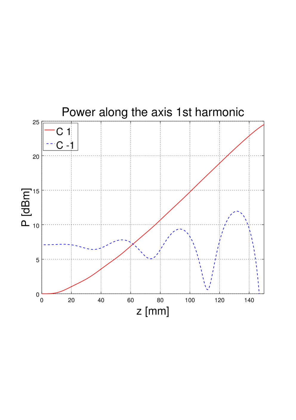
The role of backward waves is more relevant when the TWT is operated near the mode because they synchronize with the beam at this operating frequency. This is confirmed by our simulations. For this simulation, we need a much higher frequency (out of the actual operation band), at which the coupling impedance is much smaller so that amplification occurs more slowly. Near the mode, the backward wave couples efficiently with the slow space charge wave of the beam, generating the backward wave instability, where there is a risk of developing an oscillation. To stress the effect, our simulation is run without attenuation, and shows that the backward wave generated near the outlet of the TWT has an intensity exceeding significantly the input of the direct wave (here by about 8 dBm at ). So, near the mode indeed, the CoWAM must incorporate the backward wave, and a model like bwis will definitely be more accurate than mvtrad.
However, a CoWAM is unable to predict an instability if it is not foreseen by a genuine identification of the modes to be included in the run. Time-domain models will not suffer from this lack of prescience.
IV Discrete model
In contrast with the previous models, our model dimo is formulated in the time domain [3] and does not make use of the same expansion on cold fields that has been critically reviewed in section II. It implements the analysis presented in Ref. [1] and can describe any delay lines : folded waveguides, helices, coupled cavities…
We outline here the derivation of the discrete model which has been presented in detail in the past.
To take advantage of the periodicity of the slow wave structure, one first determines the solutions , to the Helmholtz equation in a periodic cell (denoted , typically , with a given profile , e.g. for a cylinder), with the Floquet boundary condition for the solenoidal (or circuit) fields , . For each propagation constant , these solutions form a basis with eigenfrequencies . Subscript labels different eigenmodes meeting the same Floquet condition, i.e. the different bands (four of them are displayed in Fig. 1).
Physical functions are expressed in terms of these eigenmodes by first applying the Gel’fand -transform [8]
| (19) | |||||
| (20) |
and expanding and on the Floquet divergence-free eigenbasis of the slow wave structure,
| (21) | |||||
| (22) |
where the first equation includes the irrotational space-charge field contribution, described with the potential , and the imaginary unit is introduced so that final physical variables of the model are purely real numbers.
This expansion is the essential difference between the discrete and the envelope models. The are the (vector) eigenfunctions of the Helmholtz equation, therefore they clearly constitute a basis on which any divergence-free vector field can be expanded at any time. The discrete model makes no approximation in the function choice. On the contrary, the expansion (1)-(2) is performed on the propagating modes at a given frequency which apparently do not necessarily constitute a basis : at a frequency below the cut-off of a waveguide, for example, evanescent modes do exist although there are no propagating modes on which they could be expanded. Even at a frequency where propagation is possible, the modes with higher cut-off frequency are still possible in the form of evanescent modes but cannot be described by the modes propagating at this frequency.
The time-dependent coefficients should generally not coincide (nor be merely proportional) as they will obey their own coupled evolution equations, whereas the envelopes in (1)-(2) had to coincide to describe the same modulation of cold fields in CoWAMs.
The Maxwell equations for the field propagation translate into evolution equations for the Floquet coefficients :
| (23) | |||||
| (24) |
where is the electromagnetic energy of mode in a unit cell of the slow wave structure, and is the beam electric current density.
Imposing a constant ratio in the discrete model (by analogy with the ’s) would be an extra condition, making the set of equations for the coefficients overdetermined. Keeping linearly independent coefficients enables the discrete model to satisfy Maxwell equations, in contrast with CoWAMs.
On introducing the field (closely related to the vector potential, see [1])
| (25) |
these equations read in real space
| (27) |
where is the full extent of the slow wave structure.
In real space and time variables, (21)-(22) give the fields in terms of these coefficients as
| (28) | |||||
| (29) |
where is the beam space charge potential.
The detailed modeling of the slow wave structures lies (i) in the frequency matrix , which is typically a band matrix , symmetric ( by reciprocity condition), with a rather short range ( if with, say, for coupled cavities [13] and for a helix), and (ii) in the explicit functions , , , whose construction involves the coupling impedances over the relevant bandwidth. As a first approximation, one mode suffices to capture the physics of the TWT. In contrast with the local picture of envelope modulation (1)-(2), the fields and should not be viewed as local to a cell but rather may have quite long a range in terms of to express how the cell couples with the beam.
The beam coupled with the wave is described by macro-electrons, with charge to mass ratio and mass , position and velocity , injected at cathode potential at a constant rate to match the physical current at the electron gun. Their equation of motion then reads
| (30) |
The space-charge potential solves the Poisson equation with particles as sources [12] and boundary conditions fixed by the slow wave structure.
V Comparison of frequency and time domain models
We now compare the cold wave amplification model in frequency domain with the discrete model in time domain. Given the experimental characteristics (dispersion diagram, coupling impedance) of the tube, we interpolated the eigenmode electric field on the axis and energy density , and constructed the matrix and interaction field defined by the Gel’fand transform.
Once again, the current modulation is obtained from a preliminary mvtrad run and is injected in equation (). This procedure permits to compare the discrete model and CoWAM with exactly the same current modulation. Indeed, these two models differ only in how electromagnetic waves are radiated from the beam, not in the dynamics of electrons given by (30).
For mvtrad and the bwis-like model respectively, we solved (14) with and , as in section III. All three models are run lossless (viz. we insert no attenuation).
Fig. 4 displays the power in the first harmonic along the tube, normalized to the input power. All three models agree qualitatively, and rather well quantitatively, for the growth of the main harmonic. Because of their richer harmonic structure, bwis and dimo show more oscillations near the entrance to the tube, but these oscillations become negligible once the field becomes so intense that the first harmonic dominates. The end of the tube was not displayed on this figure, to zoom on the region where the contrast between models is larger. The shoulder near mm is a saturation effect before the amplification resumes, and it is identically predicted by the three models, confirming their agreement.
Though these simulations were run without attenuation, dimo can accommodate these by an additional loss term in (), which becomes
| (31) |
with a localized positive time-decay rate for in cell , with the group velocity at the tube operating frequency. Runs with attenuation confirm the agreement between all three models.
VI Conclusion
We have first shown that the spatial envelope modulation assumed in CoWAMs, which made frequency models efficient for longitudinal, one-dimensional simulations, is inconsistent with the Maxwell equations in the general case. This encourages to search for alternative modelings, and the proposed discrete model is free from this failing. Moreover, since time-domain models are not restricted to a prescribed family of frequencies, they are good candidates for investigating nonlinear regimes and the appearance of unplanned resonances, such as a backward wave and drive induced oscillations.
Our second observations compare two one-dimensional CoWAMs and a simple time-domain model, dimo. On the one hand, we see that the relevant modes for a CoWAM can be reasonably predicted on the basis of their possible resonance with the beam (the backward wave is found negligible in fig. 2). On the other hand, we show that the time-domain simulation reproduces well the well-tested amplification regime where CoWAMs are reliable.
These results show the prospects opened by time-domain direct simulation using a compact discrete model with -transformed basis fields, instead of a full electromagnetic model. An improved version of dimo is currently under development, taking advantage of the explicit hamiltonian nature of particle-wave dynamics.
Acknowledgment
The authors are pleased to thank P. Bernardi, F. Doveil and D. Minenna for fruitful discussions. S. Théveny was supported by a CIFRE doctoral grant.
References
- [1] F. André, P. Bernardi, N.M. Ryskin, F. Doveil, and Y. Elskens, “Hamiltonian description of self-consistent wave-particle dynamics in a periodic structure”, Europhys. Lett., 103, 28004 (5 pp.), 2013.
- [2] F. André, P. Bernardi, N.M. Ryskin, F. Doveil, and Y. Elskens, “Hamiltonian description of the electron and its radiated field in a periodic structure”, IEEE 14th International Vacuum Electronics Conference (IVEC), 21-23 May 2013, Paris.
- [3] F. André, S. Théveny, F. Doveil, and Y. Elskens, “First comparison of new TWT discrete model with existing models”, IEEE 15th International Vacuum Electronics Conference (IVEC), 27-29 April, Beijing, 126-127, 2015.
- [4] T.M. Antonsen and B. Levush, christine : a multifrequency parametric simulation code for traveling wave tube amplifiers, Naval Research Laboratory, report number NRL/FR/6840–97-9845, Washington DC, 1997.
- [5] P. Bernardi, Utilisation et amélioration du modèle discret d’excitation d’un guide d’onde périodique pour la simulation pratique du tube à onde progressive en domaine temporel, PhD thesis, Université de Provence (Marseille), 2011.
- [6] Ch.-L. Chen, Foundations for guided-wave optics, Wiley, Hoboken NJ, 2007.
- [7] F. Doveil, D.F. Escande, and A. Macor, “Experimental observation of the nonlinear synchronization due to a single wave”, Phys. Rev. Lett., 94, 085003 (4 pp.), 2005.
- [8] S.P. Kuznetsov, “On one form of excitation equations of a periodic waveguide”, Sov. J. Commun. Technol. Electron., 25, pp. 419-421, 1980.
- [9] J. Li, Y. Mo, and Y. Zhang, “The beam-wave interaction in a Ka-band relativistic coupled-cavity TWT”, Int. J. Infrared Millimeter Waves, 25, pp. 1371-1383, 2002.
- [10] B. Li, Z.H. Yang, J.Q. Li, X.F. Zhu, T. Huang, Q. Hu, Y.L. Hu, L. Xu, J.J. Ma, L. Liao, and L. Xiao, “Theory and design of microwave-tube simulator suite”, IEEE Trans. Electron Devices, 56, pp. 919-927, 2009.
- [11] W.H. Louisell, Coupled mode and parametric electronics, Wiley, New York, 1960.
- [12] J.E. Rowe, Nonlinear electron-wave interaction phenomena, Academic Press, New York and London, 1965.
- [13] N.M. Ryskin, V.N. Titov, and A.V. Yakovlev, “Non-stationary non-linear modeling of an electron beam interaction with a coupled cavity structure, i. Theory”, in Modeling in applied electrodynamics and electronics 8, pp. 46-56, Saratov Univ. press, 2007.
- [14] P. Waller, Modélisation numérique de l’interaction et diagnostic expérimental du faisceau d’électrons dans un tube à ondes progressives spatial, PhD thesis, Université Pierre et Marie Curie (Paris), 1999.