Scaling of random walk betweenness in networks
Abstract
The betweenness centrality of graphs using random walk paths instead of geodesics is studied. A scaling collapse with no adjustable parameters is obtained as the graph size is varied; the scaling curve depends on the graph model. A normalized random betweenness, that counts each walk passing through a node only once, is also defined. It is argued to be more useful and seen to have simpler scaling behavior. In particular, the probability for a random walk on a preferential attachment graph to pass through the root node is found to tend to unity as
I Introduction
There is a large literature on the characterization of the minimal capacity required to meet end-to-end flows in networks. This characterization is typically expressed in terms of necessary or sufficient conditions on link capacities, see [1, 2] for the single commodity and [3, 4, 5, 6] for multi-commodity flows. Alternatively, one can consider the case when the flows are as efficient as possible, i.e. along shortest paths, and capacities have to be chosen to accommodate them. Depending on the structure of a network, the number of such shortest paths that pass through a node can differ substantially from node to node. As an obvious example, if two halves of a network are linked by a narrow ‘bridge’, a large number of shortest paths will pass through the bridge. A more subtle example is that of ‘hyperlattices’ or hyperbolic networks [7], where despite the absence of such a bridge, shortest paths coalesce disproportionately near the center or core of the network [8, 9]. In social networks, if one considers the shortest paths between all source-destination pairs of nodes in the network, the number of paths passing through a node is referred to as the “betweenness centrality” or betweenness of the node [10], and is a global measure of the connectivity at the node. For communications networks, this quantity usually measures the load or congestion at the node due to unit end-to-end flows. Although the physical significance of the two is different, they are the same except when there are multiple shortest paths between node pairs [11].
There are natural settings in which one might deviate from shortest path routing. Longer paths may be used for load balancing by going around highly loaded regions. In the case of capacitated networks, departures from shortest path routing can avoid network expansion. In order to study the behavior of networks when shortest path routing is no longer used, it is useful to consider its opposite extreme, random walk routing.
To be specific, we consider a graph with nodes, with the same rate of traffic flow between all possible source-destination pairs. The dynamics are discrete time. At every time step, one packet of traffic is injected at each node for each other node as destination. Any packet of traffic that was already in the graph moves randomly with equal probability to one of the adjoining nodes. If a packet reaches its destination, it is removed from the network at the next time step. The network is assumed to consist of one connected component.
Random walks on networks have been studied earlier using the graph Laplacian [12, 13] with methods similar to those we will use in this paper, but the quantities studied are different. In particular, Ref. [13] defines a random walk centrality by computing the average time to travel from a source to a destination node, and the change when the source and destination are reversed. We use alternative definitions in this paper. Ref. [12] investigates the spectral gap of the graph Laplacian.
With random walk routing, it is no longer definite whether a path from a source to a destination will pass through some node; each node has a probability of being on the path. Also, the load and the betweenness centrality are no longer equivalent. This is because a random walk wandering through the network can pass through a node several times. While it is appropriate to count each of these traversals as contributing one unit to the load at the node, it is unreasonable to consider them as each adding to the betweenness of the node.
In a separate paper [14], we have shown that the load at each node with random walk routing is linearly dependent on the degree of the node, with a proportionality constant involving the sum of the inverses of the non-zero eigenvalues of the Laplacian on the graph. We computed how the proportionality constant scales with for various network models. In this paper, we consider different ways to define the random walk betweenness of the nodes and the scaling thereof for various network models.
In the next section of this paper, we consider the definition of the random walk betweenness due to Newman [15]. We obtain an expression for this quantity in terms of the eigenfunctions of the Laplacian, from which we numerically obtain the distribution of random betweenness as a function of the number of nodes in the network. By mapping the random walk problem to current flowing in an electrical circuit, a prescription to achieve a scaling collapse of the distribution is obtained and verified for simple lattice graphs such as square and triangular lattices. This relies on the fact that the continuum limit for current flow on these graphs is diffusion on a plane. Surprisingly, the same prescription works for Erdos Renyi [16] and extended Barabasi Albert [17] graphs even though there is no underlying continuum limit. Thus for all the graph models, a scaling collapse is obtained with no adjustable parameters, using only the measured average distance between node pairs in a -node graph. The scaling form fails for hyperbolic grids — discretizations of the Poincare disk — implying that it is not trivially true.
In Section III we present an alternative definition of the random walk betweenness that we argue is more appropriate, in that a random walk contributes only once to the betweenness of every node it passes through, regardless of the number of times it does so. With this definition, an even simpler scaling collapse is obtained for the betweenness distribution as a function of the graph size
II Random walk betweenness
As in Ref. [15], we consider the random walk process described in the Introduction: with discrete time dynamics, one random walker is injected into the network at time at each source node for each other destination node; thus there are walkers injected at each node at each time step. Any walker that is present at node at time is removed from the network at time if is its destination. If not, one of the neighbors of is chosen randomly, and the walker moves there at time The probability of choosing each of the neighbors of is where is the degree of the ’th node. Note that a walker that returns to its source as it moves around randomly continues as it would from any other node.
For any given source node and destination node the net time-averaged current through each of the edges connected to a node is computed, and the magnitudes of all these are added. After adding the magnitudes of the net currents for the edges connecting to node the result is averaged over all source nodes and destination nodes to define the random walk betweenness of With this definition, if a random walk that reaches node moves out at the next time step to node through the edge and returns to through the edge at a later time, the outward flow along and the return along cancel each other. However, if the random walk leaves the node along the edge and returns later through a different edge the two do not cancel out, but are instead added. Although this definition only partially cancels the effect of a random walk looping through a node multiple times, it has the advantage that it can be mapped to an electrical circuit and solved using Kirchoff’s laws [15].
To obtain an analytical expression for the random walk betweenness, we follow the approach of Ref. [14]. For the source and destination let be the number of walkers at node at time averaged over all the random paths that the walkers can take. Let be the adjacency matrix of the graph. Then
| (1) |
The first term on the right hand side accounts for the fact that one walker is injected at node for destination at each time step. The second term represents the walkers that move to node at time from adjacent nodes at time The sum in this term excludes the node because any walker that was at the node (the destination) at time is removed from the network and is no longer present at time
We define In other words, except for the destination node, where The sum in Eq.(1) can now be unrestricted for The rate equation for the ’s is
| (2) |
for with the boundary condition
In steady state, we know that the load flowing into the node at any time step must be equal to the load injected into the node i.e. unity. Therefore and we can extend Eq.(2) in steady state as
| (3) |
for all This is a degenerate set of equations because the matrix has zero determinant; if is a solution to the equation, so is for any Therefore, even though the node is in the domain of validity of Eq.(3) unlike (2), we can still impose the condition
In order to convert Eq.(3) to a Hermitean eigenvalue problem, we define and Then
| (4) |
with Here is the Laplacian for the graph. Since is a real symmetric matrix, it has a complete set of real eigenvalues and real orthonormal eigenvectors for Using the standard properties of the graph Laplacian, all the eigenvalues are non-negative, and since the graph has been assumed to have one component, there is only one zero eigenvalue with normalized eigenvector Projecting both sides of Eq.(4) onto each eigenvector (note that the projection of the right hand side onto is zero), one can verify that
| (5) |
where remains to be determined from the condition Since is independent of we have
| (6) |
The net inflow to any node from a neighbor is then Adding the magnitudes of the currents along all the edges attached to the node (with an extra factor of half),
| (7) |
where the second term on the right hand side is due to the current flowing into and out of the graph at the nodes and respectively. The random walk betweenness of the node is then obtained by averaging over all possible sources and destinations
| (8) |
Using Eq.(6), this yields
| (9) |
The sum over on the right hand side would be equivalent to a linear combination of matrix elements of if the matrix were invertible, but it is not. To circumvent this problem, we define the operator where is the projection operator onto the zero eigenvector of the Laplacian: Unlike the Laplacian, is invertible, and
| (10) |
and therefore
| (11) |
Numerical results are obtained for various models using Eq.(11).
Before concluding this subsection, we expand on the electrical circuit analogy [15]. For any graph, one can construct a corresponding electrical circuit, where each edge is replaced by a unit resistor. Instead of one has to obtain the voltage at each node , The condition from Kirchoff’s laws is that for except nodes where current enters or leaves the graph, where is summed over nearest neighbors of But this is identical to the condition on the ’s in the random walk version of the problem, since the net flow of walkers along the edge is equal to and there is no net inflow in steady state at any node except the source or the destination. Thus to obtain the random walk betweenness of a node we inject one unit of current at node in the circuit and extract it at node add the magnitudes of the currents flowing through all the resistors connected to and average over and (with an extra factor of half and an additive correction of ).
II.1 Numerical results
We first consider square and triangular lattice graphs with overall shapes that are square and triangular respectively. Thus the square lattice graphs have nodes and the triangular lattice graphs have nodes, with various values of The random walk betweenness of all the nodes in a graph are sorted in decreasing order to obtain the distribution of random betweenness for that graph.
One can view the graph as a discretization of a continuum square or triangular surface. As is increased, the mesh size is reduced instead of the size of the surface being increased. When one unit of current is injected at one point and extracted at another, as is increased, the current density approaches the form for a continuum surface, which we denote by In order to obtain the current distribution for the lattice graph from this continuum limit, we observe that the continuum current flowing through a line segment of length that is normal to the current flow at a point is and the number of resistors in the lattice graph that cut through the line segment is Since the current is distributed over these resistors, the current in any one resistor is If we sort the nodes according to their betweenness, from the greatest to the least, in the limit, the location of the ’th node will only depend on the ratio With the nodes thus reordered, the sorted random walk betweenness should have the scaling form This argument can be generalized for a dimensional lattice, yielding
| (12) |
Numerical results for the square and triangular lattice are shown in Figure 1, and bear out this argument.
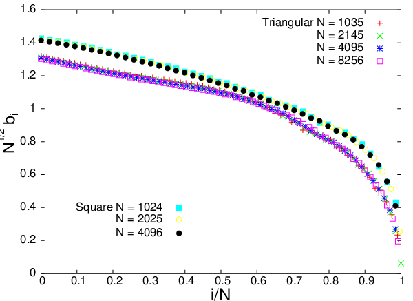
An alternative equivalent form of this result uses the fact that the average shortest path length between two randomly chosen nodes in the graph is so that
| (13) |
This form can be tested for all graphs, including those for which there is no concept of discretization of a continuum manifold, and is found to work there even though the argument given above does not apply.
We first consider Erdos Renyi [16] random graphs. For any pair of nodes in the graph, the probability of their being connected by an edge is is then the average nodal degree in the graph. There is also a dense regime for the Erdos Renyi model, where is proportional to in contrast to the sparse regime where is -independent. Because we require that the graph should have a single component, only the giant component of each graph is retained.
If the sorted random betweenness is plotted, there are large fluctuations in the plot. This is due to the randomness in how the graphs are constructed. In order to obtain a good scaling collapse, eighty graph realizations are constructed for each and the betweenness of the ’th sorted node is averaged over these realizations before a scaling collapse using Eq.(13) is attempted. (For large the number of nodes in the giant component of the graph tends to a definite fraction of in the sparse regime, and less than in the dense regime. Scaling plots are therefore constructed with rather than the actual number of nodes in the giant component.)
The average distance between nodes is found numerically for each Thus there are no adjustable parameters in the scaling plot. The results for in the sparse regime and in the dense regime are shown in Figure 2. Despite the fact that the justification given for Eq.(13) for square and triangular lattices is not applicable here, a good scaling collapse is seen.

Now we turn to preferential attachment graphs. Following the extension of Ref. [18] to the model of Ref. [17], nodes in the network are created one by one, with each node born with edges that link it to preexisting nodes. The probability of linking to a preexisting node of degree is proportional to where is a paramter of the model. As for Erdos Renyi graphs, eighty realizations were constructed for each choice of graph parameters. Again, although there is no obvious reason why the arguments leading to Eq.(13) should apply, the scaling collapse is very good for all the cases shown in Figure 3.

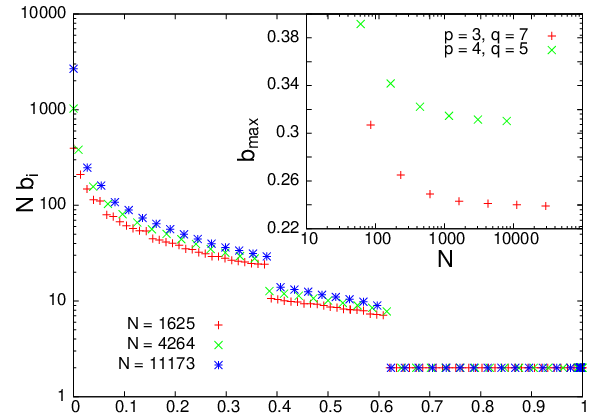
The scaling of the sorted random betweenness has implications for the node for which the random betweenness is maximum. From Figure 1, the function is seen to have a well defined limit for the square and triangular lattices. This implies that The situation is more complicated for Erdos Renyi graphs; from the inset to Figure 2, the function is seen to diverge logarithmically when its argument is small, at least in the sparse regime. This implies that does not scale as If one plots versus one observes an apparent power law form with an exponent that only depends on whether one is in the dense (average degree ) or sparse (average degree independent of ) regime. For preferential attachment graphs, Figure 3 shows that has a power law form when its argument is small, with an exponent that changes when or changes. This means that — ignoring the weak -dependence in — the maximum random walk betweenness scales as a power of with an exponent that depends on If one plots versus this is found to be the case with an exponent that only depends on
Finally, we consider the distribution of random walk betweenness for hyperbolic grids, which are tilings of the Poincare disk [7]. For these graphs, it is not possible to obtain a scaling collapse of the form given in Eq.(13): is seen to be when is comparable to but is independent of when is small. The maximum random betweenness approaches a limiting value as for these graphs. Despite the fact that these graphs are discretizations of the Poincare disk, unlike the square and triangular lattices, the underlying continuous surface has negative curvature. As a result, it is not possible to consider hyperbolic grids with different ’s as being discretizations of the same continuous region but with different mesh sizes, and the argument leading to Eq.(13) fails.
III Normalized random walk betweenness
The random walk betweenness defined in Ref. [15] and studied in the previous section ensures that if a random walk goes back and forth between two nodes, this does not increase their betweenness. However, if the walk goes round a loop repeatedly, the betweenness of all the nodes in the loop is increased by unity for each round-trip. If one is interested in finding whether a node lies in the path of many random walks, it would appear to be better to define the betweenness so that each random walk contributes exactly once to the nodes it passes through, regardless of how many times it passes through them. This quantity can be studied using the technique of the previous section, with a slight modification. To avoid confusion, we call this quantity the normalized random walk betweenness.
As before, we consider random walkers from a source node to a destination node and try to obtain the normalized random betweenness of some query node At every time step, one walker is injected into the network at the node If the walker reaches the destination node or the query node it disappears from the network at the next time step. Clearly, any random walk that reaches before it reaches contributes once to the extinction at the ’th node, even if it would have gone through multiple times before reaching if it had been allowed to continue. Any node that reaches without having gone through does not contribute to the extinction at Thus the rate at which walkers are destroyed at the node is the probability that a random walker from to will pass at least once through
In steady state, in place of Eq.(3), we have
| (14) |
where is the rate at which random walkers from to reach (for the first time), which has to be determined self-consistently. Eq.(14) comes with the boundary conditions
With we obtain the solution
| (15) |
Applying the condition we obtain
| (16) |
which fixes
| (17) |
Note that as it should be. The expression for is indeterminate; we fix it to be 1.
In order to obtain the normalized random walk betweenness of the node we average over all and with fixed. Thus
| (18) |
In the numerator, the sum over can be made unrestricted, because if Since for we have
| (19) |
Therefore
| (20) | |||||
Using Eq.(10) we have
| (21) |
from which
| (22) |
where we have replaced the subscript with to match the expression for the random walk betweenness in Section II.
III.1 Numerical results

Eq.(22) was used to numerically evaluate the normalized random walk betweenness for various models. As in Section II, the values for all the nodes in a graph were sorted. For the random graph models, the sorted list was averaged over eighty realizations of the random graph. Figure 5 shows the normalized random walk betweenness for preferential attachment networks, the Erdos Renyi model in the sparse regime, and lattice graphs. For all these cases, is only a function of For clarity, the figure only shows one example of each class of graph models, but a similar data collapse (to different curves) is seen if the model parameters are varied. For the Erdos Renyi model in the dense regime, the scaling collapse is imperfect, as shown in Figure 6.

In Figure 5, we see that the maximum normalized betweenness is close to 1 for the preferential attachment graphs. In fact, as seen in Figure 7, as for these models. This may seem surprising: implies that all the random walks pass through some node. When shortest path routing is used instead of random walks, this is impossible, and one might expect even less ‘focusing’ on any node with random walk routing.

To understand how this could happen, we consider a simpler graph: a regular tree that descends levels from a root node. Except at the lowest level, each node is connected to nodes at the next level. With randomly chosen source and destination nodes and , we calculate the probability that a random walk from to will pass through the root node. Let be the common ancestor of and When the random walk first reaches we have to calculate the probability that, thereafter, it reaches the root node before it reaches its destination. To obtain this probability, all we really need is the straight line path from the root node through to all other parts of the tree are detours, which affect the time it takes to reach the root node or its destination, but not the probability. For a random walk on this straight line, it is easy to calculate that the desired probability to reach the root node first is is where is the distance between nodes and The probability distribution for is so that is typically Then for large the probability distribution for is so that is also typically Then Therefore the probability that a random walk between randomly chosen source and destination nodes passes through the root node is
From Figure 7 we see that the root node is even more central for random walks on preferential attachment graphs than on trees, with Also surprising is the observation that is not unity for Erdos-Renyi graphs even though they are locally tree-like.
IV Conclusions
To summarize, we have considered two definitions of the random walk betweenness of the nodes in a graph: an unnormalized version which can be represented in terms of currents flowing in an electrical circuit, and a normalized version which does not measure the number of passes for a random walk through a node but instead uses a binary measure that denotes passage. For both cases, we obtain a parameter free scaling collapse of the distribution of node betweenness as a function of the size of the graph, for several graph models — with the exception of hyperbolic grids. The scaling function is singular for scale-free graphs, resulting in the maximum unnormalized betweenness being of the form with nontrivial values for Although the scaling collapse can be understood for lattice graphs through a continuum limit, it is not clear why it works for random graph models.
V Acknowledgements
Acknowledgements.
This work was supported by grants FA9550-11-1-0278 and 60NANB10D128 from AFOSR and NIST, respectively.References
- [1] L.R. Ford and D.R. Fulkerson, Canadian Jour. of Math 8:399-404 (1956).
- [2] P. Elias, A. Feinstein, C. Shannon, IEEE Trans on Information Theory 2(4):117-119 (1956).
- [3] M.V. Lomonosov, Disc Applied Math 11: 1-94 (1985).
- [4] F. Shahrokhi and D.W. Matula, Jour. of ACM 37(2): 318-334 (1990).
- [5] B.A. Papernov, Studies in Discrete Optimization (Russian), A. A. Friedman, ed. New York, pp. 17-34 (1990).
- [6] H. Okamura H and P.D. Seymour, Jour of Comb Theory, Series B 31:75-81 (1981).
- [7] R. Rietman, B. Nienhuist, J. Oitmaa, J. Phys. A: Math Gen. 25, 6577-6592 (1992).
- [8] O. Narayan and I. Saniee, Phys. Rev. E 82, 036102 (2010).
- [9] E.A. Jonckeere, M. Lou, F. Bonahon and Y. Baryshnikov, Internet Math. 7, 1 (2011).
- [10] A. Bavelas, Human Org. 7, 16 (1948); J.M. Anthonisse, The rush in a directed graph, Tech. Rep. BN 9/71, Stiching Math. Centrum (Amsterdam, 1971); L.C. Freeman, Sociometry 40, 35 (1977).
- [11] U. Brandes, Soc. Netw. 30, 136 (2008).
- [12] A.N. Samukhin, S.N. Dorogovtsev and J.F.F. Mendes Phys. Rev. E 77, 036115 (2008).
- [13] J.D. Noh and H. Rieger, Phys. Rev. Lett. 92, 118701 (2004).
- [14] O. Narayan, I. Saniee and V. Marbukh, preprint.
- [15] M.E.J. Newman, SIAM Review 45, 167 (2003).
- [16] P. Erdos and A. Renyi, Publicationes Mathematicae 6, 290 (1959).
- [17] A.-L. Barabasi and R. Albert, Science 286, 509 (1999).
- [18] S.N. Dorogovtsev, J.F.F. Mendes and A.N. Samukhin, Phys. Rev. Lett. 85, 4633 (2000).