跳到论文正文
W Papers独立论文阅读器 arXiv:1606.09288 论文正文 计算阅读时间 · 0%
引用这篇论文根据当前论文元数据生成,正式投稿前建议核对。


License: arXiv.org perpetual non-exclusive license
arXiv:1606.09288v1 [math.ST] 29 Jun 2016

Parameter estimation based on cumulative Kullback-Leibler divergence

Yaser Mehrali    Majid AsadiDepartment of Statistics, University of Isfahan, Isfahan, 81744, Iran    E-mail: yasermehrali@gmail.com, m.asadi@sci.ui.ac.ir
Abstract

In this paper, we propose some estimators for the parameters of a statistical model based on Kullback-Leibler divergence of the survival function in continuous setting. We prove that the proposed estimators are subclass of ”generalized estimating equations”estimators. The asymptotic properties of the estimators such as consistency, asymptotic normality, asymptotic confidence interval and asymptotic hypothesis testing are investigated.

Key words and Phrases: Entropy, Estimation, Generalized Estimating Equations, Information Measures.

2010 Mathematics Subject Classification: 62B10, 94A15, 94A17, 62G30, 62E20, 62F03, 62F05, 62F10, 62F12, 62F25.

1 Introduction

The Kullback-Leibler (K​LKL) divergence or relative entropy is a measure of discrimination between two probability distributions. If XX and YY have probability density functions ff and gg, respectively, the K​LKL divergence of ff relative to gg is defined as

D(f||g)=∫ℝf(x)logf⁡(x)g⁡(x)dx,D\left(f||g\right)=\int\limits_{\mathbb{R}}f\left(x\right)\log\frac{f\left(x\right)}{g\left(x\right)}dx,

for xx such that g⁡(x)≠0g(x)\not=0. The function D(f||g)D\left(f||g\right) is always nonnegative and it is zero if and only if f=gf=g a.s.a.s..

Let f⁡(x,𝜽)f\left(x;\mbox{\boldmath$\theta$}\right) belong to a parametric family with kk-dimensional parameter vector 𝜽∈𝚯⊂ℝk\mbox{\boldmath$\theta$}\in\mathbf{\Theta\subset\mathbb{R}}^{k} and fnf_{n} be kernel density estimation of ff based on nn random variables {X1,…,Xn}\{X_{1},\ldots,X_{n}\} of distribution XX. Basu and Lindsay (1994) used K​LKL divergence of fnf_{n} relative to ff\, as

D(fn||f)=∫fn(x)logfn​(x)f⁡(x,𝜽)dx,D\left(f_{n}||f\right)=\int f_{n}\left(x\right)\log\frac{f_{n}\left(x\right)}{f\left(x;\mbox{\boldmath$\theta$}\right)}dx, (1)

and defined the minimum K​LKL divergence estimator of 𝜽\theta as

𝜽^=arginf𝜽∈𝚯D(fn(x)||f(x;𝜽)).\widehat{\mbox{\boldmath$\theta$}}=\arg\underset{\mbox{\boldmath$\theta$}\in\mathbf{\Theta}}{\inf}D\left(f_{n}\left(x\right)||f\left(x;\mbox{\boldmath$\theta$}\right)\right).

Lindsay (1994) proposed a version of (1) in discrete setting. In recent years, many authors such as Morales et al. (1995), Jiménz and Shao (2001), Broniatowski and Keziou (2009), Broniatowski (2014), Cherfi (2011); Cherfi (2012); Cherfi (2014) studied the properties of minimum divergence estimators under different conditions. Basu et al. (2011) discussed in their book about the statistical inference with the minimum distance approach.

Although the method of estimation based on D(fn||f)D\left(f_{n}||f\right) has very interesting features, the definition is based on ff which, in general, may not exist and also depends on fnf_{n} which even if the number of samples tends to infinity, there is no guarantee that converges to its true measure.

Let XX be a random variable with cumulative distribution function (c.d.fc.d.f) F⁡(x)F(x) and survival function (s.fs.f) F¯​(x)\bar{F}\left(x\right). Based on nn observations {X1,…,Xn}\{X_{1},\ldots,X_{n}\} of distribution FF\,, define the empirical cumulative distribution and survival functions, respectively, by

Fn​(x)=∑i=1nin​I[X(i),X(i+1))​(x),F_{n}\left(x\right)=\sum_{i=1}^{n}\frac{i}{n}I_{\left[X_{\left(i\right)},X_{\left(i+1\right)}\right)}\left(x\right), (2)

and

F¯n​(x)=∑i=0n−1(1−in)​I[X(i),X(i+1))​(x),\bar{F}_{n}\left(x\right)=\sum_{i=0}^{n-1}\left(1-\frac{i}{n}\right)I_{\left[X_{\left(i\right)},X_{\left(i+1\right)}\right)}\left(x\right), (3)

where II is the indicator function and (0=X(0)≤)​X(1)≤X(2)≤⋯≤X(n)(0=X_{(0)}\leq)X_{(1)}\leq X_{(2)}\leq\cdots\leq X_{(n)} are the ordered sample. Fn​(F¯n)F_{n}(\bar{F}_{n}) is known in the literature as ”empirical estimator” of F⁡(F¯)F(\bar{F}).

In the case when XX and YY are continuous nonnegative random variables with s.fs.f’s F¯\bar{F} and G¯\bar{G}, respectively, a version of K​LKL in terms of s.fs.f’s F¯\bar{F} and G¯\bar{G} can be given as follows:

K​L​S​(F¯|G¯)=∫0∞F¯​(x)​log⁡F¯​(x)G¯​(x)​𝑑x−[E⁡(X)−E⁡(Y)].KLS\left(\bar{F}|\bar{G}\right)=\int_{0}^{\infty}\bar{F}\left(x\right)\log\frac{\bar{F}\left(x\right)}{\bar{G}(x)}dx-\left[E\left(X\right)-E\left(Y\right)\right].

The properties of this divergence measure are studied by some authors such as Liu (2007) and Baratpour and Habibi Rad (2012).

In order to estimate the parameters of the model, Liu (2007) proposed cumulative K​LKL divergence between the empirical survival function F¯n\bar{F}_{n} and survival function F¯\bar{F} (we call it CKL(F¯n||F¯)CKL\left(\bar{F}_{n}||\bar{F}\right)) as

CKL(F¯n||F¯)\displaystyle CKL\left(\bar{F}_{n}||\bar{F}\right) =∫0∞F¯n​(x)​log⁡F¯n​(x)F¯​(x,𝜽)−[F¯n​(x)−F¯​(x,𝜽)]​𝑑x\displaystyle=\int\nolimits_{0}^{\infty}\bar{F}_{n}\left(x\right)\log\frac{\bar{F}_{n}\left(x\right)}{\bar{F}\left(x;\mbox{\boldmath$\theta$}\right)}-\left[\bar{F}_{n}\left(x\right)-\bar{F}\left(x;\mbox{\boldmath$\theta$}\right)\right]dx
=∫0∞F¯n​(x)​log​F¯n​(x)​𝑑x−∫0∞F¯n​(x)​log​F¯​(x,𝜽)​𝑑x−[x¯−E𝜽​(X)].\displaystyle=\int\nolimits_{0}^{\infty}\bar{F}_{n}\left(x\right)\log\bar{F}_{n}\left(x\right)dx-\int\nolimits_{0}^{\infty}\bar{F}_{n}\left(x\right)\log\bar{F}\left(x;\mbox{\boldmath$\theta$}\right)dx-\left[\bar{x}-E_{\mbox{\boldmath$\theta$}}\left(X\right)\right].

The cited author defined minimum C​K​LCKL divergence estimator (M​C​K​L​EMCKLE) of 𝜽\theta as

𝜽^=arginf𝜽∈𝚯CKL(F¯n(x)||F¯(x;𝜽)).\widehat{\mbox{\boldmath$\theta$}}=\arg\underset{\mbox{\boldmath$\theta$}\in\mathbf{\Theta}}{\inf}CKL\left(\bar{F}_{n}\left(x\right)||\bar{F}\left(x;\mbox{\boldmath$\theta$}\right)\right).

If consider the parts of CKL(F¯n||F¯)CKL\left(\bar{F}_{n}||\bar{F}\right) that depends on 𝜽\theta and define

g⁡(𝜽)=E𝜽​(X)−∫0∞F¯n​(x)​log⁡F¯​(x,𝜽)​𝑑x,g\left(\mbox{\boldmath$\theta$}\right)=E_{\mbox{\boldmath$\theta$}}\left(X\right)-\int\nolimits_{0}^{\infty}\bar{F}_{n}\left(x\right)\log\bar{F}\left(x;\mbox{\boldmath$\theta$}\right)dx, (4)

then the M​C​K​L​EMCKLE of 𝜽\theta can equivalently be defined by

𝜽^=arg⁡inf𝜽∈𝚯​g​(𝜽).\widehat{\mbox{\boldmath$\theta$}}=\arg\underset{\mbox{\boldmath$\theta$}\in\mathbf{\Theta}}{\inf}g\left(\mbox{\boldmath$\theta$}\right).

Two important advantages of this estimator are that one does not need to have the density function and for large values of nn the empirical estimator FnF_{n} tends to the distribution function FF. Liu (2007) applied this estimator in uniform and exponential models and Yari and Saghafi (2012) and Yari et al. (2013) used it for estimating parameters of Weibull distribution; see also Park et al. (2012) and Hwang and Park (2013). Yari et al. (2013) found a simple form of (4) as

g⁡(𝜽)=E𝜽​(X)−1n​∑i=1nh⁡(xi)=E𝜽​(X)−h⁡(x)¯,g\left(\mbox{\boldmath$\theta$}\right)=E_{\mbox{\boldmath$\theta$}}\left(X\right)-\frac{1}{n}\sum_{i=1}^{n}h\left(x_{i}\right)=E_{\mbox{\boldmath$\theta$}}\left(X\right)-\overline{h\left(x\right)}, (5)

where h⁡(x)¯=1n​∑i=1nh⁡(xi)\overline{h\left(x\right)}=\frac{1}{n}\sum_{i=1}^{n}h\left(x_{i}\right) for any function hh on xx, and

h⁡(x)=∫0xlog⁡F¯​(y,𝜽)​𝑑y.h\left(x\right)=\int\nolimits_{0}^{x}\log\bar{F}\left(y;\mbox{\boldmath$\theta$}\right)dy. (6)

They also proved that

E⁡(h⁡(X))=∫0∞F¯​(x,𝜽)​log⁡F¯​(x,𝜽)​𝑑x,E\left(h\left(X\right)\right)=\int\nolimits_{0}^{\infty}\bar{F}\left(x;\mbox{\boldmath$\theta$}\right)\log\bar{F}\left(x;\mbox{\boldmath$\theta$}\right)dx,

which shows that if nn tends to infinity, then CKL(F¯n||F¯)CKL\left(\bar{F}_{n}||\bar{F}\right) converges to zero.

The aim of the present paper is to investigate properties of M​C​K​L​EMCKLE. The rest of the paper is organized as follows: In section 2, we propose an extension of the M​C​K​L​EMCKLE in the case when the support of the distribution is real line and provide some examples. In Section 3, we show that the proposed estimator is in the class of generalized estimating equations (G​E​EGEE). Asymptotic properties of M​C​K​L​EMCKLE such as consistency, normality are investigated in this section. In Section 3, we also provide some asymptotic confidence intervals and asymptotic tests statistics based on M​C​K​L​EMCKLE to make some inference on the parameters of the distribution.

2 An Extension of M​C​K​L​EMCKLE

In this section, we propose an extension of the M​C​K​L​EMCKLE for the case when XX is assumed to be a continuous random variable with support ℝ\mathbb{R}. It is known that

E𝜽​|X|=∫−∞0F⁡(x)​𝑑x+∫0∞F¯​(x)​𝑑x,E_{\mbox{\boldmath$\theta$}}\left|X\right|=\int\nolimits_{-\infty}^{0}F\left(x\right)dx+\int\nolimits_{0}^{\infty}\bar{F}\left(x\right)dx,

(Rohatgi and Saleh, 2015, see,).

We define the C​K​LCKL divergence and C​K​LCKL estimator in Liu approach as follows.

Definition 1.

Let XX and YY be random variables on ℝ\mathbb{R} with c.d.fc.d.f’s F⁡(x)F\left(x\right) and G⁡(x)G\left(x\right), s.fs.f’s F¯​(x)\bar{F}\left(x\right) and G¯​(x)\bar{G}\left(x\right), finite means E⁡(X)E\left(X\right) and E⁡(Y)E\left(Y\right), respectively. The C​K​LCKL divergence of F¯\bar{F} relative to G¯\bar{G} is defined as

CKL(F¯||G¯)\displaystyle CKL\left(\bar{F}||\bar{G}\right) =∫−∞0{F⁡(x)​log⁡F⁡(x)G⁡(x)−[F⁡(x)−G⁡(x)]}​𝑑x\displaystyle=\int\nolimits_{-\infty}^{0}\left\{F\left(x\right)\log\frac{F\left(x\right)}{G\left(x\right)}-\left[F\left(x\right)-G\left(x\right)\right]\right\}dx
+∫0∞{F¯(x)logF¯​(x)G¯​(x)−[F¯(x)−G¯(x)]}dx\displaystyle+\int\nolimits_{0}^{\infty}\left\{\bar{F}\left(x\right)\log\frac{\bar{F}\left(x\right)}{\bar{G}\left(x\right)}-\left[\bar{F}\left(x\right)-\bar{G}\left(x\right)\right]\right\}dx
=∫−∞0F⁡(x)​log​F⁡(x)G⁡(x)​𝑑x+∫0∞F¯​(x)​log​F¯​(x)G¯​(x)​𝑑x−[E​|X|−E​|Y|].\displaystyle=\int\nolimits_{-\infty}^{0}F\left(x\right)\log\frac{F\left(x\right)}{G\left(x\right)}dx+\int\nolimits_{0}^{\infty}\bar{F}\left(x\right)\log\frac{\bar{F}\left(x\right)}{\bar{G}\left(x\right)}dx-\left[E\left|X\right|-E\left|Y\right|\right].

An application of the log-sum inequality and the fact that x​log⁡xy≥x−y,∀x,y>0x\log\frac{x}{y}\geq x-y,\forall x,y>0 (equality holds if and only if x=yx=y) show that the C​K​LCKL is non-negative. Using the fact that in log-sum inequality, equality holds if and only if F=GF=G, a.s.a.s., one gets that CKL(F¯||G¯)=0CKL\left(\bar{F}||\bar{G}\right)=0 if and only if F=GF=G, a.s.a.s. .

Let F⁡(x,𝜽)F\left(x;\mbox{\boldmath$\theta$}\right) be the population c.d.f.c.d.f. with unknown parameters 𝜽\theta and Fn​(x)F_{n}\left(x\right) be the empirical c.d.f.c.d.f. based on a random sample X1,X2,…,XnX_{1},X_{2},\dots,X_{n} from F⁡(x,𝜽)F\left(x;\mbox{\boldmath$\theta$}\right). Based on above definition, the C​K​LCKL divergence of F¯n\bar{F}_{n} relative to F¯\bar{F} is defined as

CKL(F¯n||F¯)=∫−∞0Fn(x)logFn​(x)F⁡(x,𝜽)dx+∫0∞F¯n(x)logF¯n​(x)F¯​(x,𝜽)dx−[|x|¯−E𝜽|X|],CKL\left(\bar{F}_{n}||\bar{F}\right)=\int\nolimits_{-\infty}^{0}F_{n}\left(x\right)\log\frac{F_{n}\left(x\right)}{F\left(x;\mbox{\boldmath$\theta$}\right)}dx+\int\nolimits_{0}^{\infty}\bar{F}_{n}\left(x\right)\log\frac{\bar{F}_{n}\left(x\right)}{\bar{F}\left(x;\mbox{\boldmath$\theta$}\right)}dx-\left[\bar{\left|x\right|}-E_{\mbox{\boldmath$\theta$}}\left|X\right|\right],

where |x|¯\bar{|x|} is the mean of absolute values of the observations. Let us also define

g⁡(𝜽)=E𝜽​|X|−∫−∞0Fn​(x)​log⁡F⁡(x,𝜽)​𝑑x−∫0∞F¯n​(x)​log​F¯​(x,𝜽)​𝑑x.g\left(\mbox{\boldmath$\theta$}\right)=E_{\mbox{\boldmath$\theta$}}\left|X\right|-\int\nolimits_{-\infty}^{0}F_{n}\left(x\right)\log F\left(x;\mbox{\boldmath$\theta$}\right)dx-\int\nolimits_{0}^{\infty}\bar{F}_{n}\left(x\right)\log\bar{F}\left(x;\mbox{\boldmath$\theta$}\right)dx. (7)

If E𝜽​|X|<∞E_{\mbox{\boldmath$\theta$}}\left|X\right|<\infty and g′′​(𝜽)g^{\prime\prime}(\mbox{\boldmath$\theta$}) is positive definite, then we define M​C​K​L​EMCKLE of 𝜽\theta to be a value in the parameter space 𝚯\mathbf{\Theta} which minimizes g⁡(𝜽)g(\mbox{\boldmath$\theta$}). If k=0k=0 (i.e., XX is nonnegative), then g⁡(𝜽)g\left(\mbox{\boldmath$\theta$}\right) in (7) reduces to (4). So the results of Liu (2007), Yari and Saghafi (2012), Yari et al. (2013), Park et al. (2012) and Hwang and Park (2013) yield as special case.

It should be noted that by the law of large numbers Fn​(x)F_{n}\left(x\right) converges to F⁡(x)F\left(x\right) and F¯n​(x)\bar{F}_{n}\left(x\right) converges to F¯​(x)\bar{F}\left(x\right) as nn tends to infinity. Consequently CKL(F¯n||F¯)CKL\left(\bar{F}_{n}||\bar{F}\right) converges to zero. As a consequence, if we take 𝜽^n=T⁡(Fn)\widehat{\mbox{\boldmath$\theta$}}_{n}=T\left(F_{n}\right), then it is Fisher consistent, i.e., T⁡(F)=𝜽T\left(F\right)=\mbox{\boldmath$\theta$} (see, Fisher (1922) and Lindsay (1994)).

In order to study the properties of the estimator, we first find a simple form of (7). Let us introduce the following notations.

u⁡(x)=∫x0log⁡F⁡(y,𝜽)​𝑑y,u\left(x\right)=\int\nolimits_{x}^{0}\log F\left(y;\mbox{\boldmath$\theta$}\right)dy,

and

s⁡(x)=I(−∞,0)​(x)​u​(x)+I[0,∞)​(x)​h​(x),s\left(x\right)=I_{\left(-\infty,0\right)}\left(x\right)u\left(x\right)+I_{\left[0,\infty\right)}\left(x\right)h\left(x\right), (8)

where hh is defined in (6). Assuming that x(1),x(2),…,x(n)x_{(1)},x_{(2)},\dots,x_{(n)} denote the ordered observed values of the sample and that x(k)<0≤x(k+1)x_{\left(k\right)}<0\leq x_{\left(k+1\right)}, for some value of kk, k=0,…,nk=0,\dots,n. Then by (2), (3) and (7), we have

∫−∞0Fn​(x)​log⁡F⁡(x,𝜽)​𝑑x\displaystyle\int\nolimits_{-\infty}^{0}F_{n}\left(x\right)\log F\left(x;\mbox{\boldmath$\theta$}\right)dx =∫−∞0∑i=1nin​I[x(i),x(i+1))​(x)​log⁡F⁡(x,𝜽)​𝑑x\displaystyle=\int\nolimits_{-\infty}^{0}\sum_{i=1}^{n}\frac{i}{n}I_{\left[x_{\left(i\right)},x_{\left(i+1\right)}\right)}\left(x\right)\log F\left(x;\mbox{\boldmath$\theta$}\right)dx
=∑i=1nin​∫−∞∞I(−∞,0)​(x)​I[x(i),x(i+1))​(x)​log⁡F⁡(x,𝜽)​𝑑x\displaystyle=\sum_{i=1}^{n}\frac{i}{n}\int\nolimits_{-\infty}^{\infty}I_{\left(-\infty,0\right)}\left(x\right)I_{\left[x_{\left(i\right)},x_{\left(i+1\right)}\right)}\left(x\right)\log F\left(x;\mbox{\boldmath$\theta$}\right)dx
=∑i=1k−1in​∫x(i)x(i+1)log⁡F⁡(x,𝜽)​𝑑x+kn​∫x(k)0log⁡F⁡(x,𝜽)​𝑑x\displaystyle=\sum_{i=1}^{k-1}\frac{i}{n}\int\limits_{x_{\left(i\right)}}^{x_{\left(i+1\right)}}\log F\left(x;\mbox{\boldmath$\theta$}\right)dx+\frac{k}{n}\int\limits_{x_{\left(k\right)}}^{0}\log F\left(x;\mbox{\boldmath$\theta$}\right)dx
=1n​∑i=1k−1i⁡[u⁡(x(i))−u⁡(x(i+1))]+kn​u​(x(k))\displaystyle=\frac{1}{n}\sum_{i=1}^{k-1}i\left[u\left(x_{\left(i\right)}\right)-u\left(x_{\left(i+1\right)}\right)\right]+\frac{k}{n}u\left(x_{\left(k\right)}\right)
=1n​∑i=1k−1[i​u​(x(i))−(i+1)​u​(x(i+1))]+1n​∑i=1k−1u⁡(x(i+1))+kn​u​(x(k))\displaystyle=\frac{1}{n}\sum_{i=1}^{k-1}\left[i~u\left(x_{\left(i\right)}\right)-\left(i+1\right)u\left(x_{\left(i+1\right)}\right)\right]+\frac{1}{n}\sum_{i=1}^{k-1}u\left(x_{\left(i+1\right)}\right)+\frac{k}{n}u\left(x_{\left(k\right)}\right)
=1n​[u⁡(x(1))−k​u​(x(k))]+1n​∑i=2ku⁡(x(i))+kn​u​(x(k))\displaystyle=\frac{1}{n}\left[u\left(x_{\left(1\right)}\right)-k~u\left(x_{\left(k\right)}\right)\right]+\frac{1}{n}\sum_{i=2}^{k}u\left(x_{\left(i\right)}\right)+\frac{k}{n}u\left(x_{\left(k\right)}\right)
=1n​∑i=1ku⁡(x(i)).\displaystyle=\frac{1}{n}\sum_{i=1}^{k}u\left(x_{\left(i\right)}\right).

Using the same steps, we have

∫0∞F¯n​(x)​log⁡F¯​(x,𝜽)​𝑑x=1n​∑i=k+1nh⁡(x(i)).\int\nolimits_{0}^{\infty}\bar{F}_{n}\left(x\right)\log\bar{F}\left(x;\mbox{\boldmath$\theta$}\right)dx=\frac{1}{n}\sum_{i=k+1}^{n}h\left(x_{\left(i\right)}\right).

So g⁡(𝜽)g\left(\mbox{\boldmath$\theta$}\right) in (7) gets the simple form

g⁡(𝜽)\displaystyle g\left(\mbox{\boldmath$\theta$}\right) =E𝜽​|X|−1n​∑i=1ku⁡(x(i))−1n​∑i=k+1nh⁡(x(i))\displaystyle=E_{\mbox{\boldmath$\theta$}}\left|X\right|-\frac{1}{n}\sum_{i=1}^{k}u\left(x_{\left(i\right)}\right)-\frac{1}{n}\sum_{i=k+1}^{n}h\left(x_{\left(i\right)}\right)
=E𝜽​|X|−1n​∑i=1n[I(−∞,0)​(xi)​u​(xi)+I[0,∞)​(xi)​h​(xi)]\displaystyle=E_{\mbox{\boldmath$\theta$}}\left|X\right|-\frac{1}{n}\sum_{i=1}^{n}\left[I_{\left(-\infty,0\right)}\left(x_{i}\right)u\left(x_{i}\right)+I_{\left[0,\infty\right)}\left(x_{i}\right)h\left(x_{i}\right)\right]
=E𝜽​|X|−1n​∑i=1ns⁡(xi)=E𝜽​|X|−s⁡(x)¯.\displaystyle=E_{\mbox{\boldmath$\theta$}}\left|X\right|-\frac{1}{n}\sum_{i=1}^{n}s\left(x_{i}\right)=E_{\mbox{\boldmath$\theta$}}\left|X\right|-\overline{s\left(x\right)}. (9)

If k=0k=0 (i.e., XX is nonnegative), then g⁡(𝜽)g\left(\mbox{\boldmath$\theta$}\right) in (9) reduces to (5). It can be easily seen that

E⁡(s⁡(X))=∫−∞0F⁡(x,𝜽)​log⁡F⁡(x,𝜽)​𝑑x+∫0∞F¯​(x,𝜽)​log​F¯​(x,𝜽)​𝑑x,E\left(s\left(X\right)\right)=\int\nolimits_{-\infty}^{0}F\left(x;\mbox{\boldmath$\theta$}\right)\log F\left(x;\mbox{\boldmath$\theta$}\right)dx+\int\nolimits_{0}^{\infty}\bar{F}\left(x;\mbox{\boldmath$\theta$}\right)\log\bar{F}\left(x;\mbox{\boldmath$\theta$}\right)dx,

which proves that if nn tends to infinity, then CKL(F¯n||F¯)CKL\left(\bar{F}_{n}||\bar{F}\right) converges to zero.

In The following, we give some examples.

Example 2.

Let {X1,…,Xn}\{X_{1},\ldots,X_{n}\} be sequence of i.i.d.i.i.d. Normal random variables with probability density function

ϕ(x;μ,σ)=12​π​σ2exp(−12(x−μσ)2), x∈ℝ.\phi\left(x;\mu,\sigma\right)=\frac{1}{\sqrt{2\pi\sigma^{2}}}\exp\left(-\frac{1}{2}\left(\frac{x-\mu}{\sigma}\right)^{2}\right),\text{ \ \ \ }x\in\mathbb{R}.

In this case E⁡(|X|)=μ⁡[2​Φ​(μσ)−1]+2​σ​ϕ​(μσ)E\left(\left|X\right|\right)=\mu\left[2\Phi\left(\frac{\mu}{\sigma}\right)-1\right]+2\sigma\phi\left(\frac{\mu}{\sigma}\right), where Φ\Phi denotes the distribution function of standard normal. For this distribution, h⁡(x)h\left(x\right), u⁡(x)u\left(x\right) and g⁡(μ,σ)g\left(\mu,\sigma\right) do not have close forms. The derivative of g⁡(μ,σ)g\left(\mu,\sigma\right) with respect to μ\mu and σ\sigma and setting the results to zero gives respectively

2​n​Φ​(μσ)−n−∑i=1xi<0klog⁡Φ⁡(xi−μσ)+k​log⁡Φ⁡(−μσ)+∑i=k+1xi≥0nlog⁡Φ⁡(μ−xiσ)−(n−k)​log⁡Φ⁡(μσ)=0,2n\Phi\left(\frac{\mu}{\sigma}\right)-n-\sum_{\begin{subarray}{c}i=1\\ x_{i}<0\end{subarray}}^{k}\log\Phi\left(\frac{x_{i}-\mu}{\sigma}\right)+k\log\Phi\left(-\frac{\mu}{\sigma}\right)+\sum_{\begin{subarray}{c}i=k+1\\ x_{i}\geq 0\end{subarray}}^{n}\log\Phi\left(\frac{\mu-x_{i}}{\sigma}\right)-\left(n-k\right)\log\Phi\left(\frac{\mu}{\sigma}\right)=0,

and

2​n​ϕ​(μσ)+∑i=1xi<0k∫xi−μσ−μσz​ϕ​(z)Φ⁡(z)​𝑑z−∑i=k+1xi≥0n∫−μσxi−μσz​ϕ​(z)1−Φ⁡(z)​𝑑z=0.2n\phi\left(\frac{\mu}{\sigma}\right)+\sum_{\begin{subarray}{c}i=1\\ x_{i}<0\end{subarray}}^{k}\int\nolimits_{\frac{x_{i}-\mu}{\sigma}}^{-\frac{\mu}{\sigma}}\frac{z\phi\left(z\right)}{\Phi\left(z\right)}dz-\sum_{\begin{subarray}{c}i=k+1\\ x_{i}\geq 0\end{subarray}}^{n}\int\nolimits_{-\frac{\mu}{\sigma}}^{\frac{x_{i}-\mu}{\sigma}}\frac{z\phi\left(z\right)}{1-\Phi\left(z\right)}dz=0. (10)

To obtain our estimators, we need to solve these equations which should be solved numerically. For computational purposes, the following equivalent equation can be solved instead of (10).

2​ϕ​(μσ)+∫x(1)−μσ−μσFn​(μ+σ​z)​z​ϕ​(z)Φ⁡(z)​𝑑z−∫−μσx(n)−μσF¯n​(μ+σ​z)​z​ϕ​(z)1−Φ⁡(z)​𝑑z=0.2\phi\left(\frac{\mu}{\sigma}\right)+\int\nolimits_{\frac{x_{\left(1\right)}-\mu}{\sigma}}^{-\frac{\mu}{\sigma}}F_{n}\left(\mu+\sigma z\right)\frac{z\phi\left(z\right)}{\Phi\left(z\right)}dz-\int\nolimits_{-\frac{\mu}{\sigma}}^{\frac{x_{\left(n\right)}-\mu}{\sigma}}\bar{F}_{n}\left(\mu+\sigma z\right)\frac{z\phi\left(z\right)}{1-\Phi\left(z\right)}dz=0.

Figure 1 represents g⁡(μ,σ)g\left(\mu,\sigma\right) for a simulated sample of size 100100 from Normal distribution with parameters (μ=2,σ=3)\left(\mu=2,\sigma=3\right). This figure shows that in this case g⁡(μ,σ)g(\mu,\sigma) has minimum and hence the estimators of μ\mu and σ\sigma are the values that minimize g⁡(μ,σ)g\left(\mu,\sigma\right).

Refer to caption
Figure 1: g⁡(μ,σ)g\left(\mu,\sigma\right) for a simulated sample of size 100100 from Normal distribution with parameters (μ=2,σ=3)\left(\mu=2,\sigma=3\right)

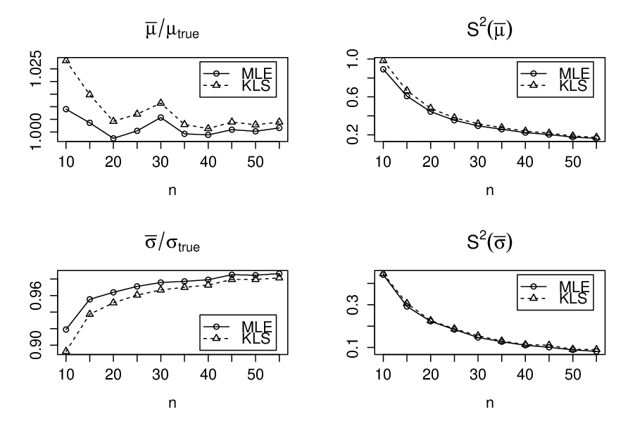
Figure 2 compares these estimators with the corresponding M​L​EMLE’s. In order to compare our estimators and the M​L​EMLE’s we made a simulation study in which we used samples of sizes 1010 to 5555 by 55 with 1000010000 repeats, where we assume that the true values of the model parameters are μt​r​u​e=2\mu_{true}=2 and σt​r​u​e=3\sigma_{true}=3. It is evident from the plots that the M​C​K​L​EMCKLE approximately coincides with the M​L​EMLE in both cases.

Refer to caption
Figure 2: μ¯/μt​r​u​e\bar{\mu}/\mu_{true}, S2​(μ¯)S^{2}\left(\bar{\mu}\right), σ¯/σt​r​u​e\bar{\sigma}/\sigma_{true} and S2​(σ¯)S^{2}\left(\bar{\sigma}\right) as functions of sample size
Example 3.

Let {X1,…,Xn}\{X_{1},\ldots,X_{n}\} be sequence of i.i.d.i.i.d. Laplace random variables with probability density function

f(x;θ)=1θexp|xθ|, x∈ℝ.f\left(x;\theta\right)=\frac{1}{\theta}\exp\left|\frac{x}{\theta}\right|,\text{ \ \ \ }x\in\mathbb{R}.

We simply have M​C​K​L​EMCKLE of θ\theta as

θ^=X2¯2.\widehat{\theta}=\sqrt{\frac{\bar{X^{2}}}{2}}.

For asymptotic properties of this estimator see Section 3.

3 Asymptotic properties of estimators

In this section we study asymptotic properties of M​C​K​L​EMCKLE’s. For this purpose, first we give a brief review on G​E​EGEE. Some related references on G​E​EGEE are Huber (1964), Serfling (1980, chapter 7), Qin and Lawless (1994), van der Vaart (2000, chapter 5), Pawitan (2001, chapter 14), Shao (2003, chapter 5), Huber and Ronchetti (2009, chapter 3) and Hampel et al. (2011).

Throughout this section, we use the terminology used by Shao (2003). We assume that X1,…,XnX_{1},...,X_{n} represents independent (not necessarily identically distributed) random vectors, in which the dimension of XiX_{i} is di,i=1,…,n⁡(supidi<∞)d_{i},~i=1,...,n~\left(\sup_{i}d_{i}<\infty\right). We also assume that in the population model the vector 𝜽\theta is a kk-vector of unknown parameters. The G​E​EGEE method is a general method in statistical inference for deriving point estimators. Let 𝚯⊂ℝk\mbox{\boldmath$\Theta$}\subset\mathbb{R}^{k} be the range of 𝜽\theta, 𝝍i\mbox{\boldmath$\psi$}_{i} be a Borel function from ℝdi×𝚯\mathbb{R}^{d_{i}}\times\mbox{\boldmath$\Theta$} to ℝk\mathbb{R}^{k}, i=1,…,ni=1,...,n, and

sn​(𝜸)=∑i=1n𝝍i​(Xi,𝜸),𝜸∈𝚯.s_{n}(\mbox{\boldmath$\gamma$})=\sum_{i=1}^{n}\mbox{\boldmath$\psi$}_{i}\left(X_{i},\mbox{\boldmath$\gamma$}\right),~\mbox{\boldmath$\gamma$}\in\mbox{\boldmath$\Theta$}.

If 𝜽^∈𝚯\widehat{\mbox{\boldmath$\theta$}}\in\mbox{\boldmath$\Theta$} is an estimator of 𝜽\theta which satisfies sn​(𝜽^)=0s_{n}(\widehat{\mbox{\boldmath$\theta$}})=0, then 𝜽^\widehat{\mbox{\boldmath$\theta$}} is called a G​E​EGEE estimator. The equation sn​(𝜸)=0s_{n}\left(\mbox{\boldmath$\gamma$}\right)=0 is called a G​E​EGEE. Most of the estimation methods such as likelihood estimators, moment estimators and M-estimators are special cases of G​E​EGEE estimators. Usually G​E​EGEE’s are chosen such that

E⁡[sn​(𝜽)]=∑i=1nE⁡[𝝍i​(Xi,𝜽)]=0.E\left[s_{n}\left(\mbox{\boldmath$\theta$}\right)\right]=\sum_{i=1}^{n}E\left[\mbox{\boldmath$\psi$}_{i}\left(X_{i},\mbox{\boldmath$\theta$}\right)\right]=0. (11)

If the exact expectation does not exist, then the expectation EE may be replaced by an asymptotic expectation. The consistency and asymptotic normality of the G​E​EGEE are studied by the authors under different conditions (Shao, 2003, see, fore example).

3.1 Consistency and asymptotic normality of the M​C​K​L​EMCKLE

Let 𝜽^n\widehat{\mbox{\boldmath$\theta$}}_{n} be M​C​K​L​EMCKLE by minimizing g⁡(𝜽)g\left(\mbox{\boldmath$\theta$}\right) in (9) with s⁡(x)s\left(x\right) as defined in (8). Here, we show that the M​C​K​L​EMCKLE’s are special cases of G​E​EGEE. Using this, we show consistency and asymptotic normality of M​C​K​L​EMCKLE’s.

Theorem 4.

M​C​K​L​EMCKLE’s, by minimizing g⁡(𝛉)g\left(\mbox{\boldmath$\theta$}\right) in (9), are special cases of G​E​EGEE estimators.

Proof:

In order to minimize g⁡(𝜽)g\left(\mbox{\boldmath$\theta$}\right) in (9), we get the derivative of g⁡(𝜽)g\left(\mbox{\boldmath$\theta$}\right), under the assumption that it exists,

∂∂𝜽​g​(𝜽)=∂∂𝜽​E𝜽​|X|−1n​∑i=1n∂∂𝜽​s​(xi)=0,\frac{\partial}{\partial\mbox{\boldmath$\theta$}}g\left(\mbox{\boldmath$\theta$}\right)=\frac{\partial}{\partial\mbox{\boldmath$\theta$}}E_{\mbox{\boldmath$\theta$}}\left|X\right|-\frac{1}{n}\sum_{i=1}^{n}\frac{\partial}{\partial\mbox{\boldmath$\theta$}}s\left(x_{i}\right)=0,

which is equivalent to G​E​EGEE sn​(𝜽)=0s_{n}\left(\mbox{\boldmath$\theta$}\right)=0 where

sn​(𝜽)=∑i=1n[∂∂𝜽​E𝜽​|X|−∂∂𝜽​s​(xi)]=∑i=1n𝝍⁡(xi,𝜽),s_{n}\left(\mbox{\boldmath$\theta$}\right)=\sum_{i=1}^{n}\left[\frac{\partial}{\partial\mbox{\boldmath$\theta$}}E_{\mbox{\boldmath$\theta$}}\left|X\right|-\frac{\partial}{\partial\mbox{\boldmath$\theta$}}s\left(x_{i}\right)\right]=\sum_{i=1}^{n}\mbox{\boldmath$\psi$}\left(x_{i},\mbox{\boldmath$\theta$}\right), (12)

with

𝝍⁡(x,𝜽)=∂∂𝜽​E𝜽​|X|−∂∂𝜽​s​(x).\mbox{\boldmath$\psi$}\left(x,\mbox{\boldmath$\theta$}\right)=\frac{\partial}{\partial\mbox{\boldmath$\theta$}}E_{\mbox{\boldmath$\theta$}}\left|X\right|-\frac{\partial}{\partial\mbox{\boldmath$\theta$}}s\left(x\right). (13)

We must prove that E​[sn​(𝜽)]=0E\left[s_{n}\left(\mbox{\boldmath$\theta$}\right)\right]=0 or equivalently E⁡[𝝍⁡(X,𝜽)]=0E\left[\mbox{\boldmath$\psi$}\left(X,\mbox{\boldmath$\theta$}\right)\right]=0. We have

E⁡[𝝍⁡(X,𝜽)]=∂∂𝜽​E𝜽​|X|−E⁡[∂∂𝜽​s​(X)].E\left[\mbox{\boldmath$\psi$}\left(X,\mbox{\boldmath$\theta$}\right)\right]=\frac{\partial}{\partial\mbox{\boldmath$\theta$}}E_{\mbox{\boldmath$\theta$}}\left|X\right|-E\left[\frac{\partial}{\partial\mbox{\boldmath$\theta$}}s\left(X\right)\right].

So, it is enough to show that

E⁡[∂∂𝜽​s​(X)]=∂∂𝜽​E𝜽​|X|.E\left[\frac{\partial}{\partial\mbox{\boldmath$\theta$}}s\left(X\right)\right]=\frac{\partial}{\partial\mbox{\boldmath$\theta$}}E_{\mbox{\boldmath$\theta$}}\left|X\right|.

By simple algebra we have

E⁡[∂∂𝜽​s​(X)]\displaystyle E\left[\frac{\partial}{\partial\mbox{\boldmath$\theta$}}s\left(X\right)\right] =\displaystyle= ∫−∞0∂∂𝜽​u​(x)​f​(x,𝜽)​𝑑x+∫0∞∂∂𝜽​h​(x)​f​(x,𝜽)​𝑑x\displaystyle\int\nolimits_{-\infty}^{0}\frac{\partial}{\partial\mbox{\boldmath$\theta$}}u\left(x\right)f\left(x;\mbox{\boldmath$\theta$}\right)dx+\int\nolimits_{0}^{\infty}\frac{\partial}{\partial\mbox{\boldmath$\theta$}}h\left(x\right)f\left(x;\mbox{\boldmath$\theta$}\right)dx (14)
=\displaystyle= ∂∂𝜽​{∫−∞0F⁡(y,𝜽)​𝑑y+∫0∞F¯​(y,𝜽)​𝑑y}\displaystyle\frac{\partial}{\partial\mbox{\boldmath$\theta$}}\left\{\int\nolimits_{-\infty}^{0}F\left(y;\mbox{\boldmath$\theta$}\right)dy+\int\nolimits_{0}^{\infty}\bar{F}\left(y;\mbox{\boldmath$\theta$}\right)dy\right\}
=\displaystyle= ∂∂𝜽​E𝜽​|X|,\displaystyle\frac{\partial}{\partial\mbox{\boldmath$\theta$}}E_{\mbox{\boldmath$\theta$}}\left|X\right|,

which proves the result. ■\blacksquare

Corollary 5.

In special case that support of XX is ℝ+\mathbb{R}^{+}, M​C​K​L​EMCKLE is an special case of G​E​EGEE estimators, where

sn​(𝜽)=∑i=1n[∂∂𝜽​E𝜽​(X)−∂∂𝜽​h​(xi)]=∑i=1n𝝍⁡(xi,𝜽),s_{n}\left(\mbox{\boldmath$\theta$}\right)=\sum_{i=1}^{n}\left[\frac{\partial}{\partial\mbox{\boldmath$\theta$}}E_{\mbox{\boldmath$\theta$}}\left(X\right)-\frac{\partial}{\partial\mbox{\boldmath$\theta$}}h\left(x_{i}\right)\right]=\sum_{i=1}^{n}\mbox{\boldmath$\psi$}\left(x_{i},\mbox{\boldmath$\theta$}\right), (15)

with

𝝍⁡(x,𝜽)=∂∂𝜽​E𝜽​(X)−∂∂𝜽​h​(x).\mbox{\boldmath$\psi$}\left(x,\mbox{\boldmath$\theta$}\right)=\frac{\partial}{\partial\mbox{\boldmath$\theta$}}E_{\mbox{\boldmath$\theta$}}\left(X\right)-\frac{\partial}{\partial\mbox{\boldmath$\theta$}}h\left(x\right). (16)

We now study other conditions under which M​C​K​L​EMCKLE’s are consistent. For each nn, let 𝜽^n\widehat{\mbox{\boldmath$\theta$}}_{n} be an M​C​K​L​EMCKLE or equivalently a G​E​EGEE estimator, i.e., sn​(𝜽^n)=0s_{n}\left(\widehat{\mbox{\boldmath$\theta$}}_{n}\right)=0, where sn​(𝜽)s_{n}\left(\mbox{\boldmath$\theta$}\right) is defined as (12) or (15). In the next Theorem, we study the regular consistency of 𝜽^n\widehat{\mbox{\boldmath$\theta$}}_{n}.

Theorem 6.

For each nn, let 𝛉^n\widehat{\mbox{\boldmath$\theta$}}_{n} be an M​C​K​L​EMCKLE or equivalently a G​E​EGEE estimator. Suppose that 𝛙\psi which is defined in (13) or (16) is a bounded and continuous function of 𝛉\theta. Let

𝚿⁡(𝜽)=E⁡[𝝍⁡(X,𝜽)],\mbox{\boldmath$\Psi$}\left(\mbox{\boldmath$\theta$}\right)=E\left[\mbox{\boldmath$\psi$}\left(X,\mbox{\boldmath$\theta$}\right)\right],

where we assume that 𝚿′​(𝛉)\mbox{\boldmath$\Psi$}^{\prime}\left(\mbox{\boldmath$\theta$}\right) exists and is full rank. Then 𝛉^n​→𝑝​𝛉\widehat{\mbox{\boldmath$\theta$}}_{n}\overset{p}{\rightarrow}\mbox{\boldmath$\theta$}.

Proof:

The result follows from Proposition 5.2 of Shao (2003) using the fact that (11) holds. ■\blacksquare

Asymptotic normality of a consistent sequence of M​C​K​L​EMCKLE’s can be established under some conditions. We first consider the special case where 𝜽\theta is scalar and X1,…,XnX_{1},...,X_{n} are i.i.d.i.i.d. .

Theorem 7.

For each nn, let 𝛉^n\widehat{\mbox{\boldmath$\theta$}}_{n} be an M​C​K​L​EMCKLE or equivalently a G​E​EGEE estimator. Then

n​(𝜽^n−𝜽)​→𝑑​N​(0,σF2),\sqrt{n}\left(\widehat{\mbox{\boldmath$\theta$}}_{n}-\mbox{\boldmath$\theta$}\right)\overset{d}{\rightarrow}N\left(0,\sigma_{F}^{2}\right),

where σF2=A/B2\sigma_{F}^{2}=A/B^{2}, with

A=E​[∂∂𝜽​s​(X)]2−[∂∂𝜽​E𝜽​|X|]2,A=E\left[\frac{\partial}{\partial\mbox{\boldmath$\theta$}}s\left(X\right)\right]^{2}-\left[\frac{\partial}{\partial\mbox{\boldmath$\theta$}}E_{\mbox{\boldmath$\theta$}}\left|X\right|\right]^{2},

and

B=∫−∞0[∂∂𝜽​F​(x,𝜽)]2F⁡(x,𝜽)​𝑑x+∫0∞[∂∂𝜽​F¯​(x,𝜽)]2F¯​(x,𝜽)​𝑑x.B=\int\nolimits_{-\infty}^{0}\frac{\left[\frac{\partial}{\partial\mbox{\boldmath$\theta$}}F\left(x;\mbox{\boldmath$\theta$}\right)\right]^{2}}{F\left(x;\mbox{\boldmath$\theta$}\right)}dx+\int\nolimits_{0}^{\infty}\frac{\left[\frac{\partial}{\partial\mbox{\boldmath$\theta$}}\bar{F}\left(x;\mbox{\boldmath$\theta$}\right)\right]^{2}}{\bar{F}\left(x;\mbox{\boldmath$\theta$}\right)}dx.

Proof:

Using Theorem 4 we have E⁡[𝝍⁡(X,𝜽)]=0E\left[\mbox{\boldmath$\psi$}\left(X,\mbox{\boldmath$\theta$}\right)\right]=0. So if consider 𝝍\psi defined in (13)

E​[𝝍⁡(X,𝜽)]2\displaystyle E\left[\mbox{\boldmath$\psi$}\left(X,\mbox{\boldmath$\theta$}\right)\right]^{2} =V​a​r​[𝝍⁡(X,𝜽)]\displaystyle=Var\left[\mbox{\boldmath$\psi$}\left(X,\mbox{\boldmath$\theta$}\right)\right]
=V​a​r​[∂∂𝜽​E𝜽​|X|−∂∂𝜽​s​(X)]\displaystyle=Var\left[\frac{\partial}{\partial\mbox{\boldmath$\theta$}}E_{\mbox{\boldmath$\theta$}}\left|X\right|-\frac{\partial}{\partial\mbox{\boldmath$\theta$}}s\left(X\right)\right]
=V​a​r​[∂∂𝜽​s​(X)]\displaystyle=Var\left[\frac{\partial}{\partial\mbox{\boldmath$\theta$}}s\left(X\right)\right]
=E​[∂∂𝜽​s​(X)]2−E2​[∂∂𝜽​s​(X)]\displaystyle=E\left[\frac{\partial}{\partial\mbox{\boldmath$\theta$}}s\left(X\right)\right]^{2}-E^{2}\left[\frac{\partial}{\partial\mbox{\boldmath$\theta$}}s\left(X\right)\right]
=E​[∂∂𝜽​s​(X)]2−[∂∂𝜽​E𝜽​|X|]2,\displaystyle=E\left[\frac{\partial}{\partial\mbox{\boldmath$\theta$}}s\left(X\right)\right]^{2}-\left[\frac{\partial}{\partial\mbox{\boldmath$\theta$}}E_{\mbox{\boldmath$\theta$}}\left|X\right|\right]^{2},

where the last equality follows from (14). On the other hand

𝚿′​(𝜽)=∂2∂𝜽2​E𝜽​|X|−E⁡[∂2∂𝜽2​s​(X)],\mbox{\boldmath$\Psi$}^{\prime}\left(\mbox{\boldmath$\theta$}\right)=\frac{\partial^{2}}{\partial\mbox{\boldmath$\theta$}^{2}}E_{\mbox{\boldmath$\theta$}}\left|X\right|-E\left[\frac{\partial^{2}}{\partial\mbox{\boldmath$\theta$}^{2}}s\left(X\right)\right],

and

E⁡[∂2∂𝜽2​s​(X)]\displaystyle E\left[\frac{\partial^{2}}{\partial\mbox{\boldmath$\theta$}^{2}}s\left(X\right)\right] =∫−∞0∫x0∂2∂𝜽2​log⁡F⁡(y,𝜽)​𝑑y​f​(x,𝜽)​𝑑x+∫0∞∫0x∂2∂𝜽2​log​F¯​(y,𝜽)​𝑑y​f​(x,𝜽)​𝑑x\displaystyle=\int_{-\infty}^{0}\int\nolimits_{x}^{0}\frac{\partial^{2}}{\partial\mbox{\boldmath$\theta$}^{2}}\log F\left(y;\mbox{\boldmath$\theta$}\right)dyf\left(x;\mbox{\boldmath$\theta$}\right)dx+\int\nolimits_{0}^{\infty}\int\nolimits_{0}^{x}\frac{\partial^{2}}{\partial\mbox{\boldmath$\theta$}^{2}}\log\bar{F}\left(y;\mbox{\boldmath$\theta$}\right)dyf\left(x;\mbox{\boldmath$\theta$}\right)dx
=∫−∞0{∂2∂𝜽2​F​(y,𝜽)F⁡(y,𝜽)−[∂∂𝜽​F​(y,𝜽)F⁡(y,𝜽)]2}​F​(y,𝜽)​𝑑y\displaystyle=\int_{-\infty}^{0}\left\{\frac{\frac{\partial^{2}}{\partial\mbox{\boldmath$\theta$}^{2}}F\left(y;\mbox{\boldmath$\theta$}\right)}{F\left(y;\mbox{\boldmath$\theta$}\right)}-\left[\frac{\frac{\partial}{\partial\mbox{\boldmath$\theta$}}F\left(y;\mbox{\boldmath$\theta$}\right)}{F\left(y;\mbox{\boldmath$\theta$}\right)}\right]^{2}\right\}F\left(y;\mbox{\boldmath$\theta$}\right)dy
+∫0∞{∂2∂𝜽2​F¯​(y,𝜽)F¯​(y,𝜽)−[∂∂𝜽​F¯​(y,𝜽)F¯​(y,𝜽)]2}F¯(y;𝜽)dy\displaystyle+\int\nolimits_{0}^{\infty}\left\{\frac{\frac{\partial^{2}}{\partial\mbox{\boldmath$\theta$}^{2}}\bar{F}\left(y;\mbox{\boldmath$\theta$}\right)}{\bar{F}\left(y;\mbox{\boldmath$\theta$}\right)}-\left[\frac{\frac{\partial}{\partial\mbox{\boldmath$\theta$}}\bar{F}\left(y;\mbox{\boldmath$\theta$}\right)}{\bar{F}\left(y;\mbox{\boldmath$\theta$}\right)}\right]^{2}\right\}\bar{F}\left(y;\mbox{\boldmath$\theta$}\right)dy
=∂2∂𝜽2​∫−∞0F⁡(x,𝜽)​𝑑x−∫−∞0[∂∂𝜽​F​(x,𝜽)]2F⁡(x,𝜽)​𝑑x\displaystyle=\frac{\partial^{2}}{\partial\mbox{\boldmath$\theta$}^{2}}\int_{-\infty}^{0}F\left(x;\mbox{\boldmath$\theta$}\right)dx-\int_{-\infty}^{0}\frac{\left[\frac{\partial}{\partial\mbox{\boldmath$\theta$}}F\left(x;\mbox{\boldmath$\theta$}\right)\right]^{2}}{F\left(x;\mbox{\boldmath$\theta$}\right)}dx
+∂2∂𝜽2∫0∞F¯(x;𝜽)dx−∫0∞[∂∂𝜽​F¯​(x,𝜽)]2F¯​(x,𝜽)dx\displaystyle+\frac{\partial^{2}}{\partial\mbox{\boldmath$\theta$}^{2}}\int\nolimits_{0}^{\infty}\bar{F}\left(x;\mbox{\boldmath$\theta$}\right)dx-\int\nolimits_{0}^{\infty}\frac{\left[\frac{\partial}{\partial\mbox{\boldmath$\theta$}}\bar{F}\left(x;\mbox{\boldmath$\theta$}\right)\right]^{2}}{\bar{F}\left(x;\mbox{\boldmath$\theta$}\right)}dx
=∂2∂𝜽2​E𝜽​|X|−∫−∞0[∂∂𝜽​F​(x,𝜽)]2F⁡(x,𝜽)​𝑑x−∫0∞[∂∂𝜽​F¯​(x,𝜽)]2F¯​(x,𝜽)​𝑑x.\displaystyle=\frac{\partial^{2}}{\partial\mbox{\boldmath$\theta$}^{2}}E_{\mbox{\boldmath$\theta$}}\left|X\right|-\int_{-\infty}^{0}\frac{\left[\frac{\partial}{\partial\mbox{\boldmath$\theta$}}F\left(x;\mbox{\boldmath$\theta$}\right)\right]^{2}}{F\left(x;\mbox{\boldmath$\theta$}\right)}dx-\int\nolimits_{0}^{\infty}\frac{\left[\frac{\partial}{\partial\mbox{\boldmath$\theta$}}\bar{F}\left(x;\mbox{\boldmath$\theta$}\right)\right]^{2}}{\bar{F}\left(x;\mbox{\boldmath$\theta$}\right)}dx.

So

𝚿′​(𝜽)=∫−∞0[∂∂𝜽​F​(x,𝜽)]2F⁡(x,𝜽)​𝑑x+∫0∞[∂∂𝜽​F¯​(x,𝜽)]2F¯​(x,𝜽)​𝑑x.\mbox{\boldmath$\Psi$}^{\prime}\left(\mbox{\boldmath$\theta$}\right)=\int_{-\infty}^{0}\frac{\left[\frac{\partial}{\partial\mbox{\boldmath$\theta$}}F\left(x;\mbox{\boldmath$\theta$}\right)\right]^{2}}{F\left(x;\mbox{\boldmath$\theta$}\right)}dx+\int\nolimits_{0}^{\infty}\frac{\left[\frac{\partial}{\partial\mbox{\boldmath$\theta$}}\bar{F}\left(x;\mbox{\boldmath$\theta$}\right)\right]^{2}}{\bar{F}\left(x;\mbox{\boldmath$\theta$}\right)}dx.

Now, using Theorem 5.13 of Shao (2003), σF2\sigma_{F}^{2} will be found. ■\blacksquare

The next Theorem shows asymptotic normality of M​C​K​L​EMCKLE’s, when 𝜽\theta is vector and X1,…,XnX_{1},...,X_{n} are i.i.d.i.i.d. .

Theorem 8.

Under the conditions of Theorem 5.14 of Shao (2003),

Vn−1/2(𝜽^n−𝜽)→𝑑Nk(0,Ik),V_{n}^{-1/2}\left(\widehat{\mbox{\boldmath$\theta$}}_{n}-\mbox{\boldmath$\theta$}\right)\overset{d}{\rightarrow}N_{k}\left(0,I_{k}\right),

where Vn=1n​B−1​A​B−1V_{n}=\frac{1}{n}B^{-1}AB^{-1} with

A=[∂∂𝜽​s​(X)]​[∂∂𝜽​s​(X)]T−[∂∂𝜽​E𝜽​|X|]​[∂∂𝜽​E𝜽​|X|]T,A=\left[\frac{\partial}{\partial\mbox{\boldmath$\theta$}}s\left(X\right)\right]\left[\frac{\partial}{\partial\mbox{\boldmath$\theta$}}s\left(X\right)\right]^{T}-\left[\frac{\partial}{\partial\mbox{\boldmath$\theta$}}E_{\mbox{\boldmath$\theta$}}\left|X\right|\right]\left[\frac{\partial}{\partial\mbox{\boldmath$\theta$}}E_{\mbox{\boldmath$\theta$}}\left|X\right|\right]^{T},

and

B=∫−∞0[∂∂𝜽​F​(x,𝜽)]​[∂∂𝜽​F​(x,𝜽)]TF⁡(x,𝜽)​𝑑x+∫0∞[∂∂𝜽​F¯​(x,𝜽)]​[∂∂𝜽​F¯​(x,𝜽)]TF¯​(x,𝜽)​𝑑x,B=\int\nolimits_{-\infty}^{0}\frac{\left[\frac{\partial}{\partial\mbox{\boldmath$\theta$}}F\left(x;\mbox{\boldmath$\theta$}\right)\right]\left[\frac{\partial}{\partial\mbox{\boldmath$\theta$}}F\left(x;\mbox{\boldmath$\theta$}\right)\right]^{T}}{F\left(x;\mbox{\boldmath$\theta$}\right)}dx+\int\nolimits_{0}^{\infty}\frac{\left[\frac{\partial}{\partial\mbox{\boldmath$\theta$}}\bar{F}\left(x;\mbox{\boldmath$\theta$}\right)\right]\left[\frac{\partial}{\partial\mbox{\boldmath$\theta$}}\bar{F}\left(x;\mbox{\boldmath$\theta$}\right)\right]^{T}}{\bar{F}\left(x;\mbox{\boldmath$\theta$}\right)}dx,

provided that BB is invertible matrix.

Proof:

The proof is similar to that of Theorem 7. ■\blacksquare

Remark 9.

In Theorems 7 and 8, for special case that support of XX is ℝ+\mathbb{R}^{+}, AA and BB are given, respectively, by

A=E​[∂∂𝜽​h​(X)]2−[∂∂𝜽​E𝜽​(X)]2,A=E\left[\frac{\partial}{\partial\mbox{\boldmath$\theta$}}h\left(X\right)\right]^{2}-\left[\frac{\partial}{\partial\mbox{\boldmath$\theta$}}E_{\mbox{\boldmath$\theta$}}\left(X\right)\right]^{2},
B=∫0∞[∂∂𝜽​F¯​(x,𝜽)]2F¯​(x,𝜽)​𝑑x,B=\int\nolimits_{0}^{\infty}\frac{\left[\frac{\partial}{\partial\mbox{\boldmath$\theta$}}\bar{F}\left(x;\mbox{\boldmath$\theta$}\right)\right]^{2}}{\bar{F}\left(x;\mbox{\boldmath$\theta$}\right)}dx,

and

A=E⁡[∂∂𝜽​h​(X)]​[∂∂𝜽​h​(X)]T−[∂∂𝜽​E𝜽​(X)]​[∂∂𝜽​E𝜽​(X)]T,A=E\left[\frac{\partial}{\partial\mbox{\boldmath$\theta$}}h\left(X\right)\right]\left[\frac{\partial}{\partial\mbox{\boldmath$\theta$}}h\left(X\right)\right]^{T}-\left[\frac{\partial}{\partial\mbox{\boldmath$\theta$}}E_{\mbox{\boldmath$\theta$}}\left(X\right)\right]\left[\frac{\partial}{\partial\mbox{\boldmath$\theta$}}E_{\mbox{\boldmath$\theta$}}\left(X\right)\right]^{T},
B=∫0∞[∂∂𝜽​F¯​(x,𝜽)]​[∂∂𝜽​F¯​(x,𝜽)]TF¯​(x,𝜽)​𝑑x.B=\int\nolimits_{0}^{\infty}\frac{\left[\frac{\partial}{\partial\mbox{\boldmath$\theta$}}\bar{F}\left(x;\mbox{\boldmath$\theta$}\right)\right]\left[\frac{\partial}{\partial\mbox{\boldmath$\theta$}}\bar{F}\left(x;\mbox{\boldmath$\theta$}\right)\right]^{T}}{\bar{F}\left(x;\mbox{\boldmath$\theta$}\right)}dx.

Now, following Pawitan (2001), we can find sample version of the variance formula for the M​C​K​L​EMCKLE as follows. Given x1,…,xnx_{1},...,x_{n} let

J=E^​[𝝍⁡(X,𝜽)]2=1n​∑i=1n𝝍2​(xi,𝜽^),J=\widehat{E}\left[\mbox{\boldmath$\psi$}\left(X,\mbox{\boldmath$\theta$}\right)\right]^{2}=\frac{1}{n}\sum_{i=1}^{n}\mbox{\boldmath$\psi$}^{2}\left(x_{i},\widehat{\mbox{\boldmath$\theta$}}\right), (17)

where in the vector case we would simply use 𝝍⁡(xi,𝜽^)​𝝍T​(xi,𝜽^)\mbox{\boldmath$\psi$}\left(x_{i},\widehat{\mbox{\boldmath$\theta$}}\right)\mbox{\boldmath$\psi$}^{T}\left(x_{i},\widehat{\mbox{\boldmath$\theta$}}\right) in the summation, and

I=−E^∂∂𝜽𝝍(X,𝜽)=−1n∑i=1n∂∂𝜽𝝍(xi,𝜽^).I=-\widehat{E}\frac{\partial}{\partial\mbox{\boldmath$\theta$}}\mbox{\boldmath$\psi$}\left(X,\mbox{\boldmath$\theta$}\right)=-\frac{1}{n}\sum_{i=1}^{n}\frac{\partial}{\partial\mbox{\boldmath$\theta$}}\mbox{\boldmath$\psi$}\left(x_{i},\widehat{\mbox{\boldmath$\theta$}}\right). (18)

Then, we have the following result.

Theorem 10.

Using notations defined in (17) and (18), and an application of Slutsky’s Theorem yields

V^n−1/2(𝜽^n−𝜽)→𝑑Nk(0,Ik),\widehat{V}_{n}^{-1/2}\left(\widehat{\mbox{\boldmath$\theta$}}_{n}-\mbox{\boldmath$\theta$}\right)\overset{d}{\rightarrow}N_{k}\left(0,I_{k}\right),

where

V^n=1n​I−1​J​I−1,\widehat{V}_{n}=\frac{1}{n}I^{-1}JI^{-1}, (19)

provided that II is invertible matrix, or equivalently g⁡(𝛉)g\left(\mbox{\boldmath$\theta$}\right) has infimum value on parameter space Θ\Theta.

In Theorems 7 and 8, the estimator V^n\widehat{V}_{n} is a sample version of VnV_{n}, see also Basu and Lindsay (1994). It is also known that the sample variance (19) is a robust estimation which is known as the ’sandwich’ estimator, with I−1I^{-1} as the bread and JJ the filling (Huber, 1967, see,). In likelihood approach, the quantity II is the usual observed Fisher information.

Example 11.

Let {X1,…,Xn}\{X_{1},\ldots,X_{n}\} be sequence of i.i.d.i.i.d. exponential random variables with probability density function

f(x;λ)=λe−λ​x, x>0,λ>0.f\left(x;\lambda\right)=\lambda e^{-\lambda x},\text{ \ \ \ }x>0,~\lambda>0.

We simply have M​C​K​L​EMCKLE of λ\lambda as

λ^=2X2¯.\widehat{\lambda}=\sqrt{\frac{2}{\bar{X^{2}}}}.

This estimator is function of linear combinations of xi2x_{i}^{2}’s, and so by strong law of large numbers (SLLN), λ^\widehat{\lambda} is strongly consistent for λ\lambda, as well as the M​M​EMME of λ\lambda.

Now, by CLT and delta method or using Theorem 7, one can show that

n​(λ^−λ)​→𝑑​N​(0,5​λ24),\sqrt{n}\left(\widehat{\lambda}-\lambda\right)\overset{d}{\rightarrow}N\left(0,\frac{5\lambda^{2}}{4}\right),

and n−1n^{-1} order asymptotic bias of λ^\widehat{\lambda} is 15​λ/8​n15\lambda/8n. It is well known that the M​L​EMLE of λ\lambda is λ^m=1/X¯\widehat{\lambda}_{m}=1/\bar{X} with asymptotic distribution

n​(λ^m−λ)​→𝑑​N​(0,λ2),\sqrt{n}\left(\widehat{\lambda}_{m}-\lambda\right)\overset{d}{\rightarrow}N\left(0,\lambda^{2}\right),

and n−1n^{-1} order asymptotic bias of λ^m\widehat{\lambda}_{m} is λ/n\lambda/n.

Notice that using asymptotic bias of λ^\widehat{\lambda}, we can find some unbiasing factors to improve our estimator. Since the M​L​EMLE has inverse Gamma distribution, the unbiased estimator of λ\lambda is λ^u​m=(n−1)/n​X¯\widehat{\lambda}_{um}=\left(n-1\right)/n\bar{X} (Forbes et al., 2011, see,). In Liu approach an approximately unbiased estimator of λ\lambda is

λ^u=8​n8​n+15​2X2¯.\widehat{\lambda}_{u}=\frac{8n}{8n+15}\sqrt{\frac{2}{\bar{X^{2}}}}. (20)

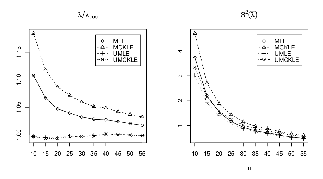
Figure 3 compares these estimators. In order to compare our estimator and the M​L​EMLE, we made a simulation study in which we used samples of sizes 1010 to 5555 by 55 with 1000010000 repeats, where we assumed that the true value of the model parameter is λt​r​u​e=5\lambda_{true}=5. The plots in Figure 3 show that the M​C​K​L​EMCKLE has more biased than the M​L​EMLE, but M​C​K​L​EMCKLE in (20) which is approximately unbiased coincides with the unbiased M​L​EMLE.

Refer to caption
Figure 3: λ¯/λt​r​u​e\bar{\lambda}/\lambda_{true} and S2​(λ¯)S^{2}\left(\bar{\lambda}\right) as functions of sample size
Remark 12.

In Example 3, note that |X|\left|X\right| has exponential distribution. So, using Example 11, one can easily find asymptotic properties of θ^\widehat{\theta} in Laplace distribution.

Example 13.

Let {X1,…,Xn}\{X_{1},\ldots,X_{n}\} be sequence of i.i.d.i.i.d. two parameter exponential random variables with probability density function

f(x;μ,σ)=1σe−(x−μ)/σ, x≥μ,μ∈ℝ,σ>0.f\left(x;\mu,\sigma\right)=\frac{1}{\sigma}e^{-\left(x-\mu\right)/\sigma},\text{ \ \ \ }x\geq\mu,~\mu\in\mathbb{R},~\sigma>0.

It is not difficult to show that M​C​K​L​EMCKLE of μ\mu and σ\sigma are, respectively,

μ^=X¯−X2¯−X¯2,σ^=X2¯−X¯2.\widehat{\mu}=\bar{X}-\sqrt{\bar{X^{2}}-\bar{X}^{2}},~\widehat{\sigma}=\sqrt{\bar{X^{2}}-\bar{X}^{2}}.

These estimators are functions of linear combinations of xix_{i}’s and xi2x_{i}^{2}’s, and hence by SLLN, (μ^,σ^)\left(\widehat{\mu},\widehat{\sigma}\right) are strongly consistent for (μ,σ)\left(\mu,\sigma\right), as well as the M​M​EMME of (μ,σ)\left(\mu,\sigma\right).

Now, by CLT and delta method or using Theorem 7, one can show that

Vn−1/2(μ^−μσ^−σ)→𝑑N2(0,I2),V_{n}^{-1/2}\left(\begin{array}[c]{c}\widehat{\mu}-\mu\\ \widehat{\sigma}-\sigma\end{array}\right)\overset{d}{\rightarrow}N_{2}\left(0,I_{2}\right),

where

Vn=σ2n​[1−1−12].V_{n}=\frac{\sigma^{2}}{n}\left[\begin{array}[c]{cc}1&-1\\ -1&2\end{array}\right].

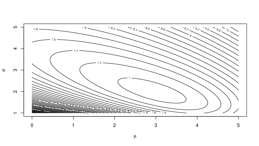
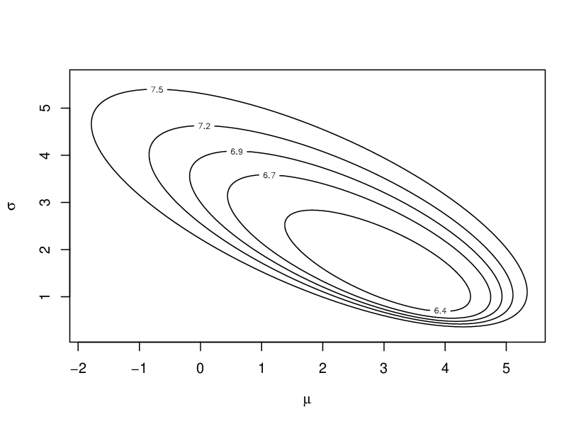
Figure 4 represents g⁡(μ,σ)g\left(\mu,\sigma\right) for a simulated sample of size 100100 from two parameter exponential distribution with parameters (μ=3,σ=2)\left(\mu=3,\sigma=2\right). The figure shows that the estimators of μ\mu and σ\sigma are the values that minimize g⁡(μ,σ)g\left(\mu,\sigma\right).

Refer to caption
Figure 4: g⁡(μ,σ)g\left(\mu,\sigma\right) for a simulated sample of size 100100 from two parameter exponential distribution with parameters (μ=3,σ=2)\left(\mu=3,\sigma=2\right)
Example 14.

Let {X1,…,Xn}\{X_{1},\ldots,X_{n}\} be sequence of i.i.d.i.i.d. Pareto random variables with probability density function

f(x;α,β)=α​βαxα+1, x≥β,α>0,β>0.f\left(x;\alpha,\beta\right)=\frac{\alpha\beta^{\alpha}}{x^{\alpha+1}},\text{ \ \ \ }x\geq\beta,~\alpha>0,~\beta>0.

So we simply have

g⁡(α,β)=α​βα−1+α​x​log⁡x¯−α​x¯​(log⁡β+1)+α​β,α>1.g\left(\alpha,\beta\right)=\frac{\alpha\beta}{\alpha-1}+\alpha\bar{x\log x}-\alpha\bar{x}\left(\log\beta+1\right)+\alpha\beta,~\alpha>1.

Differentiating g⁡(α,β)g\left(\alpha,\beta\right) with respect to β\beta and setting zero gives

β^α=x¯​(α−1)α.\widehat{\beta}_{\alpha}=\frac{\bar{x}\left(\alpha-1\right)}{\alpha}.

So, if we define the function gg of α\alpha as follows

g⁡(α)=g⁡(α,β^α)=α​x¯​log​αα−1+α​x​log⁡x¯−α​x¯​log​x¯,α>1,g\left(\alpha\right)=g\left(\alpha,\widehat{\beta}_{\alpha}\right)=\alpha\bar{x}\log\frac{\alpha}{\alpha-1}+\alpha\bar{x\log x}-\alpha\bar{x}\log\bar{x},~\alpha>1,

then, derivative of g⁡(α)g\left(\alpha\right) with respect to α\alpha and setting zero gives

log⁡αα−1−1α−1+x​log⁡x¯x¯−log⁡x¯=0.\log\frac{\alpha}{\alpha-1}-\frac{1}{\alpha-1}+\frac{\bar{x\log x}}{\bar{x}}-\log\bar{x}=0.

This equation can be solved numerically to find M​C​K​L​EMCKLE of parameters. Now, using Theorem 8, one can show that

Vn−1/2(α^−αβ^−β)→𝑑N2(0,I2),V_{n}^{-1/2}\left(\begin{array}[c]{c}\widehat{\alpha}-\alpha\\ \widehat{\beta}-\beta\end{array}\right)\overset{d}{\rightarrow}N_{2}\left(0,I_{2}\right),

where

Vn=1n​(α−2)3​[2​α​(α−1)4α​β​(α−1)2α​β​(α−1)2β2α​(α2−2​α+2)],α>2.V_{n}=\frac{1}{n\left(\alpha-2\right)^{3}}\left[\begin{array}[c]{cc}2\alpha\left(\alpha-1\right)^{4}&\alpha\beta\left(\alpha-1\right)^{2}\\ \alpha\beta\left(\alpha-1\right)^{2}&\frac{\beta^{2}}{\alpha}\left(\alpha^{2}-2\alpha+2\right)\end{array}\right],~\alpha>2.

Figure 5 represents g⁡(α,β)g\left(\alpha,\beta\right) for a simulated sample of size 100100 from Pareto distribution with parameters (α=2,β=5)\left(\alpha=2,\beta=5\right). This figure shows that the estimators of α\alpha and β\beta are the values that minimize g⁡(α,β)g\left(\alpha,\beta\right).

Refer to caption
Figure 5: g⁡(α,β)g\left(\alpha,\beta\right) for a simulated sample of size 100100 from Pareto distribution with parameters (α=2,β=5)\left(\alpha=2,\beta=5\right)

3.2 Asymptotic confidence interval

In the following we assume that 𝜽\theta is a scalar. Using Theorem 7, we can find an asymptotic confidence interval for 𝜽\theta. Under the conditions of Theorem 7, an asymptotic 100​(1−α)%100\left(1-\alpha\right)\% confidence interval for 𝜽\theta is defined as

P⁡(−zα2<n​(𝜽^−𝜽)σF<zα2)=1−α,P\left(-z_{\frac{\alpha}{2}}<\frac{\sqrt{n}\left(\widehat{\mbox{\boldmath$\theta$}}-\mbox{\boldmath$\theta$}\right)}{\sigma_{F}}<z_{\frac{\alpha}{2}}\right)=1-\alpha, (21)

where zαz_{\alpha} is the (1−α)\left(1-\alpha\right)-quantile of the N⁡(0,1)N\left(0,1\right) and σF\sigma_{F} is defined in Theorem 7. If inequalities in (21) are not invertible, then we can use σ^F\widehat{\sigma}_{F} instead of σF\sigma_{F} to obtain an approximate confidence interval, where σ^F\widehat{\sigma}_{F} is σF\sigma_{F} that evaluated at 𝜽=𝜽^\mbox{\boldmath$\theta$}=\widehat{\mbox{\boldmath$\theta$}}.

Pawitan (2001) presented an approach which is called likelihood interval for parameters. Using his approach, one can find a divergence interval for the parameter. Similar to the likelihood interval that is defined by Pawitan (2001), we define a divergence interval as a set of parameter values with low enough divergence:

{𝜽s.t.exp[g(𝜽^)−g(𝜽)]>k},\left\{\mbox{\boldmath$\theta$}\ s.t.\ \exp\left[g\left(\widehat{\mbox{\boldmath$\theta$}}\right)-g\left(\mbox{\boldmath$\theta$}\right)\right]>k\right\}, (22)

for some cutoff point kk, where exp⁡[g⁡(𝜽^)−g⁡(𝜽)]\exp\left[g\left(\widehat{\mbox{\boldmath$\theta$}}\right)-g\left(\mbox{\boldmath$\theta$}\right)\right] is the normalized divergence with g⁡(𝜽)g\left(\mbox{\boldmath$\theta$}\right) as (5) or (9); see Basu et al. (2011, chapter 5). Let us define the quantity QQ as

Q⁡(𝜽^,𝜽)=2​n​[g⁡(𝜽)−g⁡(𝜽^)]σF2⋅g′′​(𝜽^),Q\left(\widehat{\mbox{\boldmath$\theta$}},\mbox{\boldmath$\theta$}\right)=\frac{2n\left[g\left(\mbox{\boldmath$\theta$}\right)-g\left(\widehat{\mbox{\boldmath$\theta$}}\right)\right]}{\sigma_{F}^{2}\cdot g^{\prime\prime}\left(\widehat{\mbox{\boldmath$\theta$}}\right)},

where

g′′​(𝜽)=∂2∂𝜽2​g​(𝜽).g^{\prime\prime}\left(\mbox{\boldmath$\theta$}\right)=\frac{\partial^{2}}{\partial\mbox{\boldmath$\theta$}^{2}}g\left(\mbox{\boldmath$\theta$}\right).

Using Theorem 7, we show that this quantity is asymptotically a pivotal quantity. In other words, under the conditions of Theorem 7,

Q⁡(𝜽^,𝜽)​→𝑑​χ12.Q\left(\widehat{\mbox{\boldmath$\theta$}},\mbox{\boldmath$\theta$}\right)\overset{d}{\rightarrow}\chi_{1}^{2}. (23)

This is so, because using Taylor expansion of g⁡(𝜽)g\left(\mbox{\boldmath$\theta$}\right) around 𝜽^\widehat{\mbox{\boldmath$\theta$}}, we have

Q⁡(𝜽^,𝜽)≈n​(𝜽−𝜽^)2σF2.Q\left(\widehat{\mbox{\boldmath$\theta$}},\mbox{\boldmath$\theta$}\right)\approx\frac{n\left(\mbox{\boldmath$\theta$}-\widehat{\mbox{\boldmath$\theta$}}\right)^{2}}{\sigma_{F}^{2}}. (24)

Now using this fact, we can find the divergence interval for 𝜽\theta.

Theorem 15.

Under the conditions of Theorem 7, the asymptotic 100​(1−α)%100\left(1-\alpha\right)\% divergence interval for 𝛉\theta is defined as (22), with

k=exp⁡{−12​n​c​(𝜽^)​χα,12},k=\exp\left\{-\frac{1}{2n}c\left(\widehat{\mbox{\boldmath$\theta$}}\right)\chi_{\alpha,1}^{2}\right\},

where χα,12\chi_{\alpha,1}^{2} is the (1−α)\left(1-\alpha\right)-quantile of the χ12\chi_{1}^{2} and

c⁡(𝜽)=σF2⋅g′′​(𝜽).c\left(\mbox{\boldmath$\theta$}\right)=\sigma_{F}^{2}\cdot g^{\prime\prime}\left(\mbox{\boldmath$\theta$}\right).

Proof:

Using (23), the probability that divergence interval (22) covers 𝜽\theta is

P⁡(exp⁡[g⁡(𝜽^)−g⁡(𝜽)]>k)\displaystyle P\left(\exp\left[g\left(\widehat{\mbox{\boldmath$\theta$}}\right)-g\left(\mbox{\boldmath$\theta$}\right)\right]>k\right) =\displaystyle= P⁡(Q⁡(𝜽^,𝜽)<−2​n​log⁡kσF2⋅g′′​(𝜽^))\displaystyle P\left(Q\left(\widehat{\mbox{\boldmath$\theta$}},\mbox{\boldmath$\theta$}\right)<-\frac{2n\log k}{\sigma_{F}^{2}\cdot g^{\prime\prime}\left(\widehat{\mbox{\boldmath$\theta$}}\right)}\right)
=\displaystyle= P⁡(χ12<−2​n​log⁡kσF2⋅g′′​(𝜽^)).\displaystyle P\left(\chi_{1}^{2}<-\frac{2n\log k}{\sigma_{F}^{2}\cdot g^{\prime\prime}\left(\widehat{\mbox{\boldmath$\theta$}}\right)}\right).

So, for some 0<α<10<\alpha<1 we choose a cutoff

k=exp{−12​nσF2⋅g′′(𝜽^)χα,12}.k=\exp\left\{-\frac{1}{2n}\sigma_{F}^{2}\cdot g^{\prime\prime}\left(\widehat{\mbox{\boldmath$\theta$}}\right)\chi_{\alpha,1}^{2}\right\}.

Since σF2\sigma_{F}^{2} is unknown, we estimate it with σ^F2\widehat{\sigma}_{F}^{2}. This completes the proof. ■\blacksquare

Remark 16.

Form (24), The asymptotic confidence interval in (21) with σ^F\widehat{\sigma}_{F} instead of σF\sigma_{F}, is approximately equivalent with that in (22). Also, in (21) and (22), we can practically use sample version of σF2\sigma_{F}^{2} that is defined in Theorem 10.

Example 17.

In Example 11, the asymptotic 100​(1−α)%100\left(1-\alpha\right)\% divergence interval for λ\lambda is in form (22) with

k=exp⁡{−54​n​X2¯2​χα,12}.k=\exp\left\{-\frac{5}{4n}\sqrt{\frac{\bar{X^{2}}}{2}}\chi_{\alpha,1}^{2}\right\}.

In other words, the confidence interval is in form

(L,U)=b±b2−2​X2¯X2¯,\left(L,U\right)=\frac{b\pm\sqrt{b^{2}-2\bar{X^{2}}}}{\bar{X^{2}}},

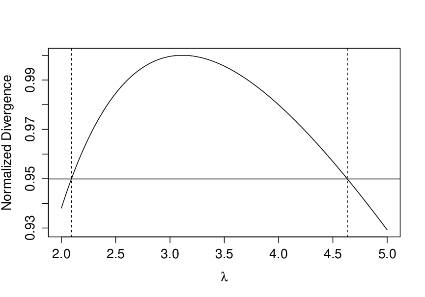
with b=−log⁡k+2​X2¯b=-\log k+\sqrt{2\bar{X^{2}}}. For a simulated sample of size n=30n=30 from exponential distribution with parameter λ=3\lambda=3, Figure 6 shows normalized divergence and asymptotic 95%95\% confidence interval for λ\lambda. In this typical sample x2¯=0.2063127\bar{x^{2}}=0.2063127, λ^=3.113522\widehat{\lambda}=3.113522, λ^u=2.930374\widehat{\lambda}_{u}=2.930374, k=0.9498908k=0.9498908 and (L,U)=(2.092375,4.633022)\left(L,U\right)=\left(2.092375,4.633022\right).

Refer to caption
Figure 6: Normalized divergence and asymptotic 95%95\% confidence interval for λ\lambda\,, in a simulated sample of size n=30n=30 from exponential distribution with parameter λ=3\lambda=3.
Remark 18.

When dim(𝜽)>1\dim\left(\mbox{\boldmath$\theta$}\right)>1, we can’t easily find a pivotal quantity. In these cases, using quantiles of g∗g^{\ast} from repeated samples, we can find cutoffs of divergence-based confidence regions.

Example 19.

In Example 13, Using 1000010000 replicated simulated samples of size 100100 from two parameter exponential distribution with parameters (μ=3,σ=2)\left(\mu=3,\sigma=2\right), we can find asymptotic cutoffs of divergence-based confidence regions for (μ,σ)\left(\mu,\sigma\right). Figure 7 shows asymptotic 90%,70%,…,10%90\%,70\%,\ldots,10\% confidence regions for (μ,σ)\left(\mu,\sigma\right).

Refer to caption
Figure 7: Asymptotic 90%,70%,…,10%90\%,70\%,\ldots,10\% confidence regions for (μ,σ)\left(\mu,\sigma\right), using 1000010000 replicated simulated samples of size 100100 from two parameter exponential distribution with parameters (μ=3,σ=2)\left(\mu=3,\sigma=2\right)

3.3 Asymptotic hypothesis testing

Let dim(𝜽)=1\dim\left(\mbox{\boldmath$\theta$}\right)=1 and 𝚯0\mathbf{\Theta}_{0} and 𝚯1\mathbf{\Theta}_{1} be two subsets of 𝚯\mathbf{\Theta} such that

𝚯0∪𝚯1=𝚯,𝚯0∩𝚯1=ϕ.\mathbf{\Theta}_{0}\cup\mathbf{\Theta}_{1}=\mathbf{\Theta,~\Theta}_{0}\cap\mathbf{\Theta}_{1}=\phi.

We are interested in testing hypotheses

H0:𝜽∈𝚯0​ vs ​H1:𝜽∈𝚯1.H_{0}:\mbox{\boldmath$\theta$}\in\mathbf{\Theta}_{0}\text{\ vs }H_{1}:\mbox{\boldmath$\theta$}\in\mathbf{\Theta}_{1}. (25)

It is clear that by inverting asymptotic confidence interval in (21), we can find a critical region for statistical tests (asymptotically of level α\alpha)

H0:𝜽=𝜽0​ vs ​H1:𝜽≠𝜽0,H_{0}:\mbox{\boldmath$\theta$}=\mbox{\boldmath$\theta$}_{0}\text{\ vs }H_{1}:\mbox{\boldmath$\theta$}\neq\mbox{\boldmath$\theta$}_{0}, (26)

for a given 𝜽0\mbox{\boldmath$\theta$}_{0}. Similar to approach of generalized likelihood ratio test, Basu (1993) and Lindsay (1994) presented a divergence difference test (D​D​T)\left(DDT\right) statistic based on (1) for testing hypotheses in (26) in continuous and discrete cases; also see Basu et al. (2011, chapter 5). Here, we perform an alternative statistical test based on C​K​LCKL divergence. For testing hypotheses in (25), we define the generalized divergence difference test (G​D​D​T)\left(GDDT\right) statistic as

G​D​D​T\displaystyle GDDT =2​n​[inf𝜽∈𝚯0​g​(𝜽)−inf𝜽∈𝚯​g​(𝜽)]\displaystyle=2n\left[\underset{\mbox{\boldmath$\theta$}\in\mathbf{\Theta}_{0}}{\inf}g\left(\mbox{\boldmath$\theta$}\right)-\underset{\mbox{\boldmath$\theta$}\in\mathbf{\Theta}}{\inf}g\left(\mbox{\boldmath$\theta$}\right)\right]
=2​n​[g⁡(𝜽^0)−g⁡(𝜽^)].\displaystyle=2n\left[g\left(\widehat{\mbox{\boldmath$\theta$}}_{0}\right)-g\left(\widehat{\mbox{\boldmath$\theta$}}\right)\right].

We consider behavior of G​D​D​TGDDT as a test statistic for a null hypothesis of the form H0:𝜽∈𝚯0H_{0}:\mbox{\boldmath$\theta$}\in\mathbf{\Theta}_{0}.

Theorem 20.

Under the conditions of Theorem 7 and the null hypothesis H0:𝛉∈𝚯0H_{0}:\mbox{\boldmath$\theta$}\in\mathbf{\Theta}_{0},

G​D​D​T​→𝑑​c​(𝜽^0)​χ12.GDDT\overset{d}{\rightarrow}c\left(\widehat{\mbox{\boldmath$\theta$}}_{0}\right)\chi_{1}^{2}.

Proof:

Using Taylor expansion of g⁡(𝜽^0)g\left(\widehat{\mbox{\boldmath$\theta$}}_{0}\right) around 𝜽^\widehat{\mbox{\boldmath$\theta$}} we get

2​n​[g⁡(𝜽^0)−g⁡(𝜽^)]\displaystyle 2n\left[g\left(\widehat{\mbox{\boldmath$\theta$}}_{0}\right)-g\left(\widehat{\mbox{\boldmath$\theta$}}\right)\right] ≈2​n​[g⁡(𝜽^)+(𝜽^0−𝜽^)​g′​(𝜽^)+(𝜽^0−𝜽^)22​g′′​(𝜽^)−g⁡(𝜽^)]\displaystyle\approx 2n\left[g\left(\widehat{\mbox{\boldmath$\theta$}}\right)+\left(\widehat{\mbox{\boldmath$\theta$}}_{0}-\widehat{\mbox{\boldmath$\theta$}}\right)g^{\prime}\left(\widehat{\mbox{\boldmath$\theta$}}\right)+\frac{\left(\widehat{\mbox{\boldmath$\theta$}}_{0}-\widehat{\mbox{\boldmath$\theta$}}\right)^{2}}{2}g^{\prime\prime}\left(\widehat{\mbox{\boldmath$\theta$}}\right)-g\left(\widehat{\mbox{\boldmath$\theta$}}\right)\right]
=n​(𝜽^0−𝜽^)22​g′′​(𝜽^).\displaystyle=\frac{n\left(\widehat{\mbox{\boldmath$\theta$}}_{0}-\widehat{\mbox{\boldmath$\theta$}}\right)^{2}}{2}g^{\prime\prime}\left(\widehat{\mbox{\boldmath$\theta$}}\right).

Under H0H_{0}, the quantity g′′​(𝜽^)g^{\prime\prime}\left(\widehat{\mbox{\boldmath$\theta$}}\right) convergence to g′′​(𝜽^0)g^{\prime\prime}\left(\widehat{\mbox{\boldmath$\theta$}}_{0}\right). Thus

G​D​D​T≈c⁡(𝜽^0)​n​(𝜽^0−𝜽^)2σF02,GDDT\approx c\left(\widehat{\mbox{\boldmath$\theta$}}_{0}\right)\frac{n\left(\widehat{\mbox{\boldmath$\theta$}}_{0}-\widehat{\mbox{\boldmath$\theta$}}\right)^{2}}{\sigma_{F_{0}}^{2}},

where σF02\sigma_{F_{0}}^{2} is σF2\sigma_{F}^{2} that evaluated at 𝜽=𝜽^0\mbox{\boldmath$\theta$}=\widehat{\mbox{\boldmath$\theta$}}_{0}. Now using Theorem 7 the proof is complete. ■\blacksquare

Remark 21.

Under the conditions of Theorem 20, we can obtain the following approximation for the power function in a given 𝜽1∈𝚯1\mbox{\boldmath$\theta$}_{1}\in\mathbf{\Theta}_{1} as

β⁡(𝜽1)≈P⁡(χ12>2​n​[g⁡(𝜽1)−g⁡(𝜽^0)]+c⁡(𝜽^0)​χα,12c⁡(𝜽1)).\beta\left(\mbox{\boldmath$\theta$}_{1}\right)\approx P\left(\chi_{1}^{2}>\frac{2n\left[g\left(\mbox{\boldmath$\theta$}_{1}\right)-g\left(\widehat{\mbox{\boldmath$\theta$}}_{0}\right)\right]+c\left(\widehat{\mbox{\boldmath$\theta$}}_{0}\right)\chi_{\alpha,1}^{2}}{c\left(\mbox{\boldmath$\theta$}_{1}\right)}\right).

As an important application of the above approximation, one can find the approximate sample size that guarantees a specific power β\beta for a given 𝜽1∈𝚯1\mbox{\boldmath$\theta$}_{1}\in\mathbf{\Theta}_{1}. Let n0n_{0} be the positive root of the equation

β=P⁡(χ12>2​n​[g⁡(𝜽1)−g⁡(𝜽^0)]+c⁡(𝜽^0)​χα,12c⁡(𝜽1)),\beta=P\left(\chi_{1}^{2}>\frac{2n\left[g\left(\mbox{\boldmath$\theta$}_{1}\right)-g\left(\widehat{\mbox{\boldmath$\theta$}}_{0}\right)\right]+c\left(\widehat{\mbox{\boldmath$\theta$}}_{0}\right)\chi_{\alpha,1}^{2}}{c\left(\mbox{\boldmath$\theta$}_{1}\right)}\right),

i.e.,

n0=c⁡(𝜽1)​χβ,12−c⁡(𝜽^0)​χα,122​[g⁡(𝜽1)−g⁡(𝜽^0)].n_{0}=\frac{c\left(\mbox{\boldmath$\theta$}_{1}\right)\chi_{\beta,1}^{2}-c\left(\widehat{\mbox{\boldmath$\theta$}}_{0}\right)\chi_{\alpha,1}^{2}}{2\left[g\left(\mbox{\boldmath$\theta$}_{1}\right)-g\left(\widehat{\mbox{\boldmath$\theta$}}_{0}\right)\right]}.

The required sample size is then

n∗=[n0]+1,n^{\ast}=\left[n_{0}\right]+1, (27)

where [⋅]\left[\cdot\right] is used here to denote ”integer part of”.

Remark 22.

In special case that 𝚯0={𝜽0}\mathbf{\Theta}_{0}=\left\{\mbox{\boldmath$\theta$}_{0}\right\}, we can find a critical region for statistical tests (asymptotically of level α\alpha) in (26). One can do this by replacing 𝜽^0\widehat{\mbox{\boldmath$\theta$}}_{0} with 𝜽0\mbox{\boldmath$\theta$}_{0}.

Example 23.

In Example 11, the statistical test (asymptotically of level α\alpha) of null hypothesis H0:λ=λ0H_{0}:\lambda=\lambda_{0} against the alternative H1:λ≠λ0H_{1}:\lambda\neq\lambda_{0} is defined with the critical region

X2¯>(b+b2−4​a​c2​a)2​ or ​X2¯<(b−b2−4​a​c2​a)2,\bar{X^{2}}>\left(\frac{b+\sqrt{b^{2}-4ac}}{2a}\right)^{2}\text{ or }\bar{X^{2}}<\left(\frac{b-\sqrt{b^{2}-4ac}}{2a}\right)^{2},

where a=n​λ02a=n\lambda_{0}^{2}, b=2​2​n​λ0b=2\sqrt{2}n\lambda_{0} and c=2​n−52​χα,12c=2n-\frac{5}{2}\chi_{\alpha,1}^{2}.

References

  • Baratpour and Habibi Rad (2012) Baratpour, S., & Habibi Rad, A. (2012). Testing goodness-of-fit for exponential distribution based on cumulative residual entropy. Communications in Statistics-Theory and Methods, 41(8), 1387-1396.
  • Basu (1993) Basu, A. (1993). Minimum disparity estimation: applications to robust tests of hypotheses. Technical Report, Center for Statistical Sciences, University of Texas at Austin.
  • Basu and Lindsay (1994) Basu, A., & Lindsay, B. G. (1994). Minimum disparity estimation for continuous models: efficiency, distributions and robustness. Annals of the Institute of Statistical Mathematics, 46(4), 683-705.
  • Basu et al. (2011) Basu, A., Shioya, H., & Park, C. (2011). Statistical inference: the minimum distance approach. CRC Press.
  • Broniatowski (2014) Broniatowski, M. (2014). Minimum divergence estimators, maximum likelihood and exponential families. Statistics & Probability Letters, 93, 27-33.
  • Broniatowski and Keziou (2009) Broniatowski, M., & Keziou, A. (2009). Parametric estimation and tests through divergences and the duality technique. Journal of Multivariate Analysis, 100(1), 16-36.
  • Cherfi (2011) Cherfi, M. (2011). Dual ϕ\phi-divergences estimation in normal models. arXiv preprint arXiv:1108.2999.
  • Cherfi (2012) Cherfi, M. (2012). Dual divergences estimation for censored survival data. Journal of Statistical Planning and Inference, 142(7), 1746-1756.
  • Cherfi (2014) Cherfi, M. (2014). On Bayesian estimation via divergences. Comptes Rendus Mathematique, 352(9), 749-754.
  • Fisher (1922) Fisher, R. A. (1922). On the mathematical foundations of theoretical statistics. Philosophical Transactions of the Royal Society of London. Series A, Containing Papers of a Mathematical or Physical Character, 222, 309-368.
  • Forbes et al. (2011) Forbes, C., Evans, M., Hastings, N., & Peacock, B. (2011). Statistical distributions. John Wiley & Sons.
  • Hampel et al. (2011) Hampel, F. R., Ronchetti, E. M., Rousseeuw, P. J., & Stahel, W. A. (2011). Robust statistics: the approach based on influence functions (Vol. 114). John Wiley & Sons.
  • Huber (1964) Huber, P. J. (1964). Robust estimation of a location parameter. The Annals of Mathematical Statistics, 35(1), 73-101.
  • Huber (1967) Huber, P. J. (1967). The behavior of maximum likelihood estimates under nonstandard conditions. Proceedings of the fifth Berkeley symposium on mathematical statistics and probability. 221-233.
  • Huber and Ronchetti (2009) Huber, P., & Ronchetti, E. (2009). Robust Statistics, Wiley: New York.
  • Hwang and Park (2013) Hwang, I., & Park, S. (2013). On scaled cumulative residual Kullback-Leibler information. Journal of the Korean Data and Information Science Society, 24(6), 1497-1501.
  • Jiménz and Shao (2001) Jiménz, R., & Shao, Y. (2001). On robustness and efficiency of minimum divergence estimators. Test, 10(2), 241-248.
  • Lindsay (1994) Lindsay, B. G. (1994). Efficiency versus robustness: the case for minimum Hellinger distance and related methods. The Annals of Statistics, 22(2), 1081-1114.
  • Liu (2007) Liu, J. (2007). Information theoretic content and probability. Ph.D. Thesis, University of Florida.
  • Morales et al. (1995) Morales, D., Pardo, L., & Vajda, I. (1995). Asymptotic divergence of estimates of discrete distributions. Journal of Statistical Planning and Inference, 48(3), 347-369.
  • Park et al. (2012) Park, S., Rao, M., & Shin, D. W. (2012). On cumulative residual Kullback–Leibler information. Statistics & Probability Letters, 82(11), 2025-2032.
  • Pawitan (2001) Pawitan, Y. (2001). In all likelihood: statistical modelling and inference using likelihood: Oxford University Press.
  • Qin and Lawless (1994) Qin, J., & Lawless, J. (1994). Empirical likelihood and general estimating equations. The Annals of Statistics, 22(1), 300-325.
  • Rohatgi and Saleh (2015) Rohatgi, V. K., & Saleh, A. M. E. (2015). An introduction to probability and statistics (2 ed.). John Wiley. New York.
  • Serfling (1980) Serfling, R. (1980). Approximation Theorems of Mathematical Statistics John Wiley. New York.
  • Shao (2003) Shao, J. (2003). Mathematical Statistics (2 ed.). Springer, New York, USA.
  • van der Vaart (2000) van der Vaart, A. W. (2000). Asymptotic statistics. Cambridge university press.
  • Yari et al. (2013) Yari, G., Mirhabibi, A., & Saghafi, A. (2013). Estimation of the Weibull parameters by Kullback-Leibler divergence of Survival functions. Appl. Math, 7(1), 187-192.
  • Yari and Saghafi (2012) Yari, G., & Saghafi, A. (2012). Unbiased Weibull Modulus Estimation Using Differential Cumulative Entropy. Communications in Statistics-Simulation and Computation, 41(8), 1372-1378.