A Semi-Definite Programming approach to low dimensional embedding for unsupervised clustering
Abstract
This paper proposes a variant of the method of Guédon and Verhynin for estimating the cluster matrix in the Mixture of Gaussians framework via Semi-Definite Programming. A clustering oriented embedding is deduced from this estimate. The procedure is suitable for very high dimensional data because it is based on pairwise distances only. Theoretical garantees are provided and an eigenvalue optimisation approach is proposed for computing the embedding. The performance of the method is illustrated via Monte Carlo experiements and comparisons with other embeddings from the literature.
1 Introduction
1.1 Motivations
Low dimensional embedding is a key to many modern data analysis procedures. The main underlying idea is that the data is better understood after extracting the main features of the samples. Based on a compressed description from a few extracted features, the individual samples can then be projected, visualized or clustered more reliably and efficiently.
The main embedding techniques available nowadays are PCA [20] and its robust version [9], random embeddings [19], (see also the recent [10] for supervised classification), Laplacian Eigenmap [4], Maximum Variance Unfolding/Semi-Definite embedding [33], …The first two techniques in this list are linear embeddings methods, whereas the other are nonlinear in nature.
In modern data science, the samples may lie in very high dimensional spaces. Our main objective in the present paper is to propose a technique for a low dimensional representation which aims at preparing the data for unsupervised clustering at the same time. Combining the goals of projecting and clustering is not new. This is achieved in particular by spectral clustering [30] [3, Chapter 3]. The SemiDefinite embedding technique in [22] is also motivated by clustering purposes. Spectral clustering is based on a Laplacian matrix constructed from the pairwise distances of the samples and whose second eigenvector is proved to separate the data into two clusters using the normalized cut criterion. The second eigenvector is called the Fiedler vector. The analysis is usually presented from the perspective of Cheeger’s relaxation and a clever randomized algorithm [3, Chapter 3]. Clustering into more than two groups can also be performed using a higher order Cheeger theory [21], a direction which has not been much explored in practice yet.
A frequent way to illustrate non-linear low dimensional embedding such as Diffusion Maps is shown in Figure 1.


In particular, the main idea in such methods is to approximately preserve the pairwise distances. Such a constraint is often inappropriate for any embedding based preconditioner for any clustering technique where one would like to concentrate the samples belonging to the same cluster and separate the samples belonging to different clusters.
In this paper, we propose a study of Guedon and Vershynin’s method for finding an embedding with clustering purposes in mind. The essential ingredient allowing to focus on clustering more than distance preserving compression/visualization is to try to estimate the clustering matrix and use spectral embedding on the cluster matrix instead of the Laplacian matrix itself. More precisely, the cluster matrix is the square matrix indexed by the data and whose entries are one if the associated data belong to the same cluster and zero otherwise. This eigenvalue decomposition of this matrix provides a perfect clustering procedure: its rank is exactly the number of clusters and each data is associated with exactly one eigenvector. Similarly to spectral clustering, the eigenvectors give a meaningful embedding. Motivated by these considerations, it seems fairly reasonable to expect that a good approximation of the clustering matrix will also provide an efficient embedding, i.e. suitable for clustering, via its eigenvalue decomposition. This intuition is supported by Remark 1.6 in [14] which we now quote: It may be convenient to view the cluster matrix as the adjacency matrix of the cluster graph, in which all vertices within each community are connected and there are no connections across the communities. This way, the semidefinite program takes a sparse graph as an input, and it returns an estimate of the cluster graph as an output. The effect of the program is thus to "densify" the network inside the communities and "sparsify" it across the communities.
Our goal here will thus be to approximate the clustering matrix efficiently, based on the knowledge of the sample pairwise distances. Guedon and Vershynin proved that such a good approximation could be found as the solution to a Semi-Definite Programming (SDP) problem for community detection in the Stochastic Block Model framework. We pursue this study here by considering the Gaussian Mixture Model framework.
1.2 Recent advances in clustering
Unsupervised clustering is a key problem in modern data analysis. Traditional approaches to clustering are model based (e.g. Gaussian mixture models) or nonparametric. For mixture models, the algorithm of choice has long been the EM algorithm by Dempster et al. [13], see the monograph by McLachlan and Peel [23] for an overview of finite mixture models. Nonparametric algorithms such as -means, -means ++ and generalizations have been used extensively in computer science; see Jain [18] for a review. The main drawback of these standard approaches is that the minimization problems underlying the various procedures are not convex. Even worse, the log-likelihood function of e.g. Gaussian mixture model exhibits degenerate behavior, see Biernacki and Chrétien [6]. As a result, one can never certify that such algorithms have converged to an interesting stationary point and the popularity of such methods seems to be based on their satisfactory average practical performance.
Recently some convex minimization based methods have been proposed in the literature. A nice method using ideas similar to the LASSO is ClusterPath [17]. This very interesting and efficient method has been studied and extended in [28], [26] and [32]. One of the main drawbacks of this approach is the lack of a robust rule for the choice of the parameters governing the procedure although they seem to be reasonably easy to tune in practice. A closely related approach is [12].
Recently, very interesting results have appeared for the closely related problem of community detection based on the stochastic block model, see Abbe et al. [1], Heimlicher et al. [15] and Mossel et al. [24]. In this model, a random graph is constructed by partitioning the set of vertices into clusters and by setting an edge between vertices and with probability if and . All edges are independent and the probabilities of edges depends only on the clusters structure. It is assumed that this probability is larger within clusters, i.e.
| (1) |
This corresponds to the intuitive notion of cluster in graph theory where clusters have a higher edge density. Guédon and Vershynin [14] proved that the problem of recovering the clusters from the random graph can be addressed via Semi-Definite Programming (SDP) with an explicit control of the error rate. Although not explicitly studied in their paper, the SDP can be solved efficiently thanks to a general theory, see Boyd and Vandenberghe [8].
1.3 More on the Gaussian Cluster Model
The mathematical framework is the following. We assume that we observe a data set over a population of size . The population is partitioned into clusters of size respectively, i.e. . We assume the standard Gaussian Cluster Model for the data: the observations are independent with
| (2) |
with the cluster mean and the cluster covariance matrix. The clustering problem aims at recovering the clusters , , based on the data , , only. For each , we will denote by the index of the cluster to which belongs. The notation will mean that and belong to the same cluster.
This slightly differs from the usual setting for Gaussian unmixing. One usually assume that the data set is made of independent observations from the mixture of Gaussian distributions
where the vector gives the mixture distribution. Then the cluster sizes are random with multinomial distribution of size and probability parameters . Given all the parameters of the Gaussian mixture, the probability that observation belongs to cluster is given by
with the Gaussian distribution function. Maximizing these probabilities results in a partition of the space into different regions given by
The probability that an observation is misclassified is then given by
Of course in practice the parameters , , are unknown and have to be estimated. The most popular approach is based on maximum likelihood estimation via the EM algorithm [13] and its variant like CEM, see Céleux and Govaert [11]. The likelihood
may behave quite badly and exhibit degenerate behavior, making optimization via EM not always reliable, see [6].
Another viewpoint on the results from the present paper is to propose a low dimensional preconditioner for the Gaussian Mixture estimation problem.
1.4 Our contribution
Firstly, we propose an extension of the analysis of Guédon and Vershynin to the problem of low dimensional embedding via the estimation of the cluster matrix with Gaussian clustering in mind. We provide in particular a theoretical upper bound for the misclassification rate. This adaptation is non trivial because, unlike the stochastic block model, the affinity matrix associated to Gaussian clustering does not have independent entries. Thus we need to introduce concentration inequalities for Gaussian measures, see e.g. the monograph by Boucheron et al. [7]. Secondly, we propose a simple and scalable algorithm to solve the Semi-Definite Program based on eigenvalue optimization in the spirit of [16]. Thirdly, we suggest a practical way of choosing the unknown parameter in the Guedon Vershynin relaxation.
1.5 Structure of the paper
The paper is organized as follows. Section 3 is devoted to the proof of Proposition 1 and Theorem 1. Section 4 provides explicit formulas for the expected affinity matrix in the case when is the Gaussian affinity function (4). An efficient algorithm is described in Section 5, as well as a practical method for selecting the unkown parameter.
2 Main results
2.1 Motivation for the cluster matrix estimation approach
The main idea is to use the fact that the cluster matrix is a very special matrix. Indeed, if we denote by , …, the index set of each cluster, we can write as follows:
and thus, we conclude that
- •
the rank of is
- •
the eigenvalues of are , …,
- •
the eigenvectors of are , …, .
In the sequel, we will assume that the cluster sizes are all different. Thus, all nonzero eigenvalues have multiplicity equal to one.
Based on the cluster matrix , clustering is very easy: the label of each sample point is the index of the only eigenvector whose component is non zero. Notice that the component of all other eigenvectors are equal to zero.
The estimate of the matrix can be used in practice to embed the data into the space by associating each data to the vector consisting of the coordinate of the first eigenvectors of . Given this embedding, if we can prove that accurately estimates , one can then apply any clustering method of choice to recover the clustering pattern of the original data. The next section gives a method for computing an estimator of .
2.2 Guedon and Vershynin’s Semi-Definite Program for Gaussian clusters
We now turn to the estimation of the cluster matrix using Guedon and Vershynin’s Semi-Definite Programming based approach. Whereas Vershynin and Guédon [14] were interested in analyzing the Stochastic Block Model for community detection, we propose a study of the Gaussian Cluster Model and therefore prove that their approach has a great potential applicability in embedding of general data sets beyond the graphical model setting.
Based on the data set , we construct an affinity matrix by
| (3) |
where denotes the Euclidean norm on and an affinity function. A popular choice is the Gaussian affinity
| (4) |
and other possibilities are
Before stating the Semi-Definite Program, we introduce some matrix notations. The usual scalar product between matrices is denoted by . The notations and stand for the vector and matrices with all entries equal to 1. For a symmetric matrix , the notation means that the quadratic form associated to is non-negative while the notation means that all the entries of are non-negative.
With these notations, the Semi-Definite Program writes
| (5) |
with the set of symmetric matrices such that
| (6) |
Let us provide some intuitions for motivating the SDP problem (5). Note that each has entries in with constant sum equal to . The SDP procedure will distribute the mass and assign more mass to entries corresponding to large values of the affinity , i.e. pairs of close points . This mass distribution must respect symmetry and the constraint . For the analysis of the procedure, the main idea is that we want the solution to be an approximation of , the cluster matrix defined by
| (7) |
The cluster matrix has values in and belongs to for given by the cluster sizes. In practice, is unknown and should be estimated, see some comment in section 5.1.5. Under some natural assumption (see Equation (10) below), the cluster matrix is the solution of the alternative SDP problem
| (8) |
where denotes the expected affinity matrix defined by
| (9) |
The affinity matrix is a very noisy observation of but concentration arguments together with Grothendieck theorem allow to prove that in the sense of the – norm. In turn, this implies (in the sense of norm) so that the SDP program (5) provides a good approximation of the cluster matrix.
2.3 Main results
Our main result provides a non asymptotic upper bound for the probability that differs from in distance.
Theorem 1.
Consider the Gaussian Cluster Model (2). Assume that the affinity function is -Lipschitz and furthermore that
| (10) |
Let
Then, for all ,
| (11) |
where denotes the Grothendieck constant and with the largest eigenvalue of the covariance matrix . Moreover, there exists a subset with such that all ,
| (12) |
Condition (10) ensures that the affinity matrix allows to identify the clusters and appears also in [14], see Eq. (1). In the case of the Gaussian affinity function (4), we provide in Section 4 explicit formulae for the expected affinity matrix that can be used to check condition (10).
Theorem 1 has a simple consequence in terms of estimation error rate. After computing , it is natural to estimate the cluster graph by a random graph obtained by putting an edge between vertices and if and no edge otherwise. Then the proportion of errors in the prediction of the edges is given by
The following corollary provides a simple bound for the asymptotic error.
Corollary 1.
We have almost surely
In the case when the cluster means are pairwise different and fixed while the cluster variances converge to , i.e. , it is easily seen that the right hand side of the above inequality behaves as so that the error rate converges to . This reflects the fact that when all clusters concentrates around their means, clustering becomes trivial.
Remark 1.
Theorem 1 assumes that is known. It is worth noting that corresponds to the number of edges in the cluster graph and that we can derive from the proof of Theorem 1 how the algorithm behaves when the cluster sizes are unknown, i.e. when the unknown parameter is replaced by a different value . The intuition is given in Remark 1.6 of Guédon and Vershynin: if , the solution will estimate a certain subgraph of the cluster graph with at most missing edges; if , the solution will estimate a certain supergraph of the cluster graph with at most extra-edges.
While our proof of Theorem 1 follows the ideas from Vershynin and Guédon [14], we need to introduce new tools to justify the approximation in -norm. Indeed, unlike in the stochastic block model, the entries of the affinity matrix (3) are not independent. We use Gaussian concentration measure arguments to obtain the following concentration inequality. The – norm of a matrix is defined by
| (13) |
Proposition 1.
Consider the Gaussian mixture model (2) and assume the affinity function is -Lipschitz. Then, for any ,
| (14) |
3 Proofs
3.1 Proof of Proposition 1
Proof.
The concentration of the affinity matrix around its mean follows from concentration inequalities for Lipschitz function of independent standard Gaussian variables, see Appendix A. From definition (13)
| (15) |
We introduce the standardized observations: if is in cluster , i.e. , then , are independent identically distributed random variables with standard Gaussian distribution. In view of definition (15), the random variables can be expressed in terms of the standardized observations
We prove next that the function is -Lipschitz with . Indeed, for , we have
In the first inequality, we use the fact that is -Lipschitz. The second inequality relies on the fact that all the eigenvalues of are smaller that . The last inequality relies on Cauchy-Schwartz inequality and on the definition .
3.2 Proof of Theorem 1
The proof follows the same lines as in Guédon and Vershynin [14] and we provide the main ideas for the sake of completeness. The proof is divided into 4 steps.
3.2.1 Step 1
We show solves the SDP problem (8). This corresponds to Lemma 7.1 in [14]. This is proved simply as follows. Since , we transform the SDP problem (8) into the simpler problem
In order to solve this second problem, the mass has to be assigned to the entries where is maximal. Thanks to (10), this corresponds exactly to the cluster matrix . One can then check a posteriori that so that in fact the original SDP problem (8) has been solved.
3.2.2 Step 2
3.2.3 Step 3
We show that for every ,
| (18) |
This corresponds to Lemma 7.2 in [14] and shows that the expected objective function distinguishes points. Introducing the set
| (19) |
of edges within clusters and the set
| (20) |
of edges across clusters, we decompose the scalar product
Note that the definition of the cluster matrix (7) implies that if and if . This together with condition (10) implies
Introduce and . Since , we have . On the other hand . We deduce exact expressions for and and the lower bound
| (21) |
3.2.4 Proof of (11)
3.2.5 Proof of (12)
4 Explicit formulæ for the expected affinity matrix
In order to check condition (10), explicit formulas for the mean affinity matrix are useful.
Proposition 2.
Assume that is build using the Gaussian affinity function (4).
- •
Let and be in the same cluster . Then,
with the eigenvalues of .
- •
Let and be in different clusters and . Then,
with and respectively the eigenvalues and eigenvectors of .
Proof.
The proof of the proposition relies on the fact that is a Gaussian random vector with mean and variance so that the distribution of is related to the noncentral distribution with degrees of freedom. The next Lemma provides the Laplace transform of the noncentral distribution.
Lemma 1.
Let . If , we have
with the eigenvalues of . More generally, for ,
with the eigenvalues of and the associated eigenvectors.
∎
Remark 2.
In dimension , we obtain the very simple formula
In the case of clusters, the condition writes
When , we simply need .
5 Computing a solution of the SDP relaxation
5.1 The algorithm
5.1.1 Further description of the constraints
The constraints that every diagonal element of should be equal to can be written as
| (26) |
The constraint can be expressed as the rank- constraint
| (27) |
where is the all-ones matrix of size .
5.1.2 Helmberg and Rendl’s spectral formulation
One of the nice features of the Semi-Definite Program (5)-(6) is that it can be rewritten as an eigenvalue optimization problem. Let us adopt a Lagrangian duality approach to this problem. As in [16], we will impose the reduntant constraint that the trace is constant. The Lagrange function is given by
Now the dual function is given by
| (28) |
Therefore, we easily get that
where is the maximum eigenvalue function. Therefore, the solution to this problem is amenable to eigenvalue optimization. An important remark is that a maximizer in (28) associated to a dual minimizer will be a solution of the original problem. It can be written as
where is a matrix whose columns form a basis of the eigenspace associated with .
5.1.3 Using the HANSO algorithm
The maximum eigenvalue is a convex function. Let denote the affine operator
The subdifferential of is given by
where is a matrix whose columns form a basis for the eigenspace associated to the maximum eigenvalue of and
where is the multiplicity of this maximum eigenvalue.
With these informations in hand, it is easy to minimize the dual function . Indeed, the subdifferential of at is simply given by
The algorithm HANSO [25] can then be used to perform the actual minimization of the dual function . A primal solution can then be recovered as a maximizer in the definition (28) of the dual function.
5.1.4 Computing the actual clustering
As advised in [31], the actual clustering can be computed using a minimum spanning tree method and removing the largest edges.
5.1.5 Choosing
6 Simulation results
In all the experiments, the parameter in (4) was chosen as
6.1 Some interesting examples
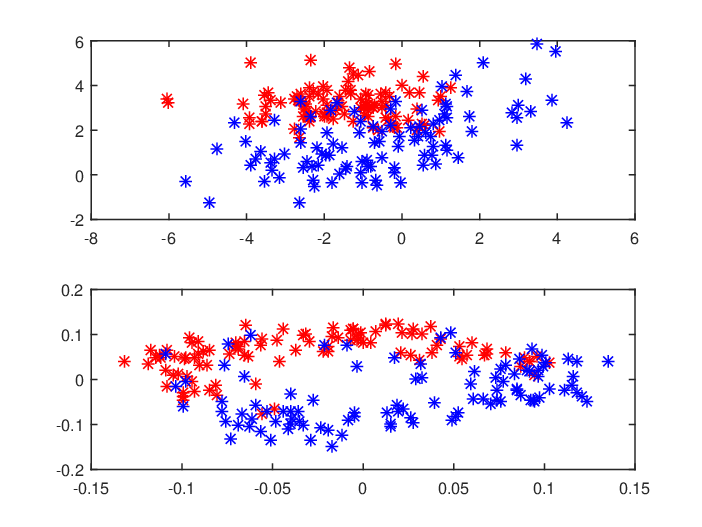
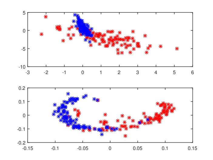
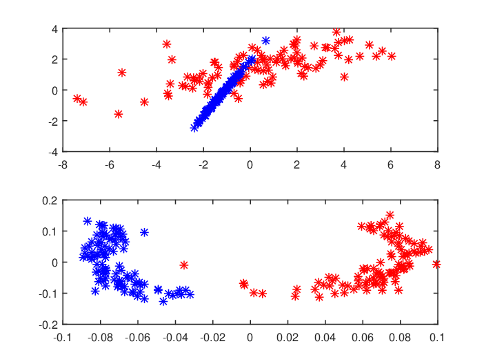
In this section, we start with three examples where the separation properties of the Guedon-Vershynin embedding are nicely illustrated. In all three instances, the data were generated using two 2- dimensional Gaussians samples with equal size (100 samples by cluster). These examples are shown in Figure 2, Figure 3 and Figure 4 below. All these example seem to be very difficult to address for methods with guaranteed polynomial time convergence. In each case, one observes that the clusters are well separated after the embedding and that they do not look like Gaussian samples anymore. The fact of not being Gaussian does not impair the success of methods such as minimum spanning trees although such methods might work better with the example in Figure 4 than in the example of Figure 2 and Figure 3.
6.2 Comparison with standard embeddings on a 3D cluster example
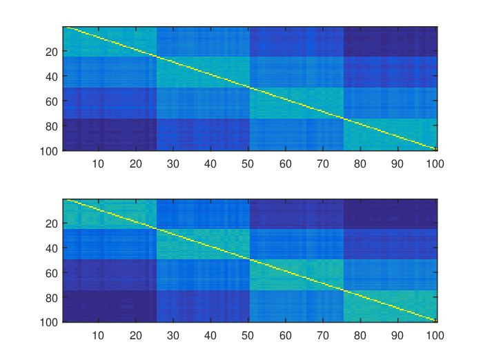
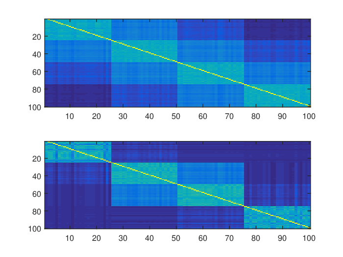
Simulations have been conducted to assess the quality of the proposed embedding. In this subsection, we used the Matlab package drtoolbox https://lvdmaaten.github.io/drtoolbox/ proposed by Laurens Van Maatten on a sample drawn from a 10 dimensional Gaussian Mixture Model with 4 components and equal proportions. In Figure 5, we show the original affinity matrix together with the estimated cluster matrix. In Figure 6, we compare the affinity matrix of data with the affinity matrix of the mapped data using various embeddings proposed in the drtoolbox package. This toy experiment shows that the embedding described in this paper can cluster as the same time as is embeds into a small dimensional subspace. This is not very surprising since our embedding is taylored for the joint clustering-dimensionality reduction purpose whereas most of the known existing embedding methods aren’t. Given the fact that clustered data are ubiquitous in real world data analysis due to the omnipresence of stratified populations, taking the clustering purpose into account might be a considerable advantage.


6.3 The sparsity of the solution
In this experiment, we computed the relative sparsity of the affinity matrix of the embedded data v.s. the sparsity of the affinity matrix of the original data.
Since the matrix is not exactly sparse, we chose to study the quasi-norm instead of the exact sparsity for small, i.e. .
We made 250 Monte Carlo experiments in dimension 10, 30, 50, 70 and 90. The histogram of the relative error of the quasi-norm for each dimension is given in Figure 7. In this experiment, we draw the sample from two Gaussian distributions with mean drawn from and covariance drawn as where the components of are i.i.d. . The affinity matrix of the orignal data is already quite sparse but the embedding improves the sparsity by 10 to nearly 20 percent as the dimension increases.


7 Conclusions
The goal of the present paper was to propose an analysis of Guedon and Vershynin’s Semi-Definite Programming approach to the estimation of the cluster matrix and show how this matrix can be used to produce an embedding for preconditionning standard clustering procedures. The procedure is suitable for very high dimensional data because it is based on pairwise distances only. Moreover, increasing the dimension will improve the robustness of the procedure as soon as a Law of Large Numbers holds along the variables instead of the samples, forcing the affinity matrix to converge to a deterministic limit and thus making the estimator less sensitive to its low dimensional fluctuations.
Another feature of the method is that it may apply to a large number of mixtures type, even when the component’s densities are not log-concave, as do a lot of embeddings as applied to data concentrated on complicated manifolds. Further studies will be performed in this exciting direction.
Future work is also needed for proving that the proposed preconditioner is provably efficient when combined with various clustering techniques. One of the main reason why this should be a difficult problem is that the approximation bound proved in the present paper, which is of the same order as for the Stochastic Block Model, is hard to use for controlling the perturbation of the eigenspaces of . More precise use of the inherent randomness of the perturbation, in the spirit of [31], might bring the necessary ingredient in order to go a little further in this direction.
Appendix A Concentration inequalities
The following inequality is a particuliar case of the Log-Sobolev concentration inequality, see Theorems 5.5 and 5.6. in [7].
Theorem 2 (Gaussian concentration inequality).
Let be independent Gaussian random vectors on with mean and variance . Assume that is Lipschitz with constant , i.e.
Then the random variable satisfies
and also
The next theorem provides result for the expected maxima of (non necessarily independent) subgaussian random variables.
Theorem 3.
Let be real valued sub-Gaussian random variables with variance factor , i.e. satisfying
Then
Appendix B The Grothendieck inequality
In this paper, we use the following matrix version of Grothendieck inequality. We denote by the set of matrices with having all raws in the unit Euclidean ball, i.e.
Theorem 4 (Grothendieck inequality).
There exists an universal constant such that every matrix satisfies
where the norm of is defined by (13).
It is also useful to note the following properties of , see Lemma 3.3 in [14].
Lemma 2.
Every matrix such that and satisfies .
References
- [1] Emmanuel Abbe, Afonso S Bandeira, and Georgina Hall, Exact recovery in the stochastic block model, arXiv preprint arXiv:1405.3267 (2014).
- [2] Hirotugu Akaike, A new look at the statistical model identification, Automatic Control, IEEE Transactions on 19 (1974), no. 6, 716–723.
- [3] Afonso S Bandeira, Ten lectures and forty-two open problems in the mathematics of data science, (2015).
- [4] Mikhail Belkin and Partha Niyogi, Laplacian eigenmaps and spectral techniques for embedding and clustering., NIPS, vol. 14, 2001, pp. 585–591.
- [5] Christophe Biernacki, Gilles Celeux, and Gérard Govaert, Assessing a mixture model for clustering with the integrated completed likelihood, Pattern Analysis and Machine Intelligence, IEEE Transactions on 22 (2000), no. 7, 719–725.
- [6] Christophe Biernacki and Stéphane Chrétien, Degeneracy in the maximum likelihood estimation of univariate gaussian mixtures with em, Statistics & probability letters 61 (2003), no. 4, 373–382.
- [7] Stéphane Boucheron, Gábor Lugosi, and Pascal Massart, Concentration inequalities, Oxford University Press, Oxford, 2013, A nonasymptotic theory of independence, With a foreword by Michel Ledoux. MR 3185193
- [8] Stephen Boyd and Lieven Vandenberghe, Convex optimization, Cambridge university press, 2004.
- [9] Emmanuel J Candès, Xiaodong Li, Yi Ma, and John Wright, Robust principal component analysis?, Journal of the ACM (JACM) 58 (2011), no. 3, 11.
- [10] Timothy I Cannings and Richard J Samworth, Random projection ensemble classification, arXiv preprint arXiv:1504.04595 (2015).
- [11] Gilles Celeux and Gérard Govaert, A classification EM algorithm for clustering and two stochastic versions, Comput. Statist. Data Anal. 14 (1992), no. 3, 315–332. MR 1192205 (93k:62126)
- [12] Gary K Chen, Eric C Chi, John Michael O Ranola, and Kenneth Lange, Convex clustering: An attractive alternative to hierarchical clustering, PLoS Comput Biol 11 (2015), no. 5, e1004228.
- [13] A. P. Dempster, N. M. Laird, and D. B. Rubin, Maximum likelihood from incomplete data via the EM algorithm, J. Roy. Statist. Soc. Ser. B 39 (1977), no. 1, 1–38, With discussion. MR 0501537 (58 #18858)
- [14] Olivier Guédon and Roman Vershynin, Community detection in sparse networks via grothendieck’s inequality, Probability Theory and Related Fields (2015), 1–25.
- [15] Simon Heimlicher, Marc Lelarge, and Laurent Massoulié, Community detection in the labelled stochastic block model, arXiv preprint arXiv:1209.2910 (2012).
- [16] Christoph Helmberg and Franz Rendl, A spectral bundle method for semidefinite programming, SIAM Journal on Optimization 10 (2000), no. 3, 673–696.
- [17] Toby Dylan Hocking, Armand Joulin, Francis Bach, and Jean-Philippe Vert, Clusterpath an algorithm for clustering using convex fusion penalties, 28th international conference on machine learning, 2011, p. 1.
- [18] Anil K Jain, Data clustering: 50 years beyond k-means, Pattern recognition letters 31 (2010), no. 8, 651–666.
- [19] William B Johnson and Joram Lindenstrauss, Extensions of lipschitz mappings into a hilbert space, Contemporary mathematics 26 (1984), no. 189-206, 1.
- [20] Ian Jolliffe, Principal component analysis, Wiley Online Library, 2002.
- [21] James R Lee, Shayan Oveis Gharan, and Luca Trevisan, Multiway spectral partitioning and higher-order cheeger inequalities, Journal of the ACM (JACM) 61 (2014), no. 6, 37.
- [22] Nathan Linial, Eran London, and Yuri Rabinovich, The geometry of graphs and some of its algorithmic applications, Combinatorica 15 (1995), no. 2, 215–245.
- [23] Geoffrey McLachlan and David Peel, Finite mixture models, John Wiley & Sons, 2004.
- [24] Elchanan Mossel, Joe Neeman, and Allan Sly, Stochastic block models and reconstruction, arXiv preprint arXiv:1202.1499 (2012).
- [25] M Overton, Hanso: a hybrid algorithm for nonsmooth optimization, Available from cs. nyu. edu/overton/software/hanso (2009).
- [26] Peter Radchenko and Gourab Mukherjee, Consistent clustering using an fusion penalty, arXiv preprint arXiv:1412.0753 (2014).
- [27] Gideon Schwarz et al., Estimating the dimension of a model, The annals of statistics 6 (1978), no. 2, 461–464.
- [28] Kean Ming Tan, Daniela Witten, et al., Statistical properties of convex clustering, Electronic Journal of Statistics 9 (2015), no. 2, 2324–2347.
- [29] Joel A Tropp, Column subset selection, matrix factorization, and eigenvalue optimization, Proceedings of the Twentieth Annual ACM-SIAM Symposium on Discrete Algorithms, Society for Industrial and Applied Mathematics, 2009, pp. 978–986.
- [30] Ulrike Von Luxburg, A tutorial on spectral clustering, Statistics and computing 17 (2007), no. 4, 395–416.
- [31] Van Vu, Singular vectors under random perturbation, Random Structures & Algorithms 39 (2011), no. 4, 526–538.
- [32] Binhuan Wang, Yilong Zhang, Wei Sun, and Yixin Fang, Sparse convex clustering, arXiv preprint arXiv:1601.04586 (2016).
- [33] Kilian Q Weinberger and Lawrence K Saul, Unsupervised learning of image manifolds by semidefinite programming, International Journal of Computer Vision 70 (2006), no. 1, 77–90.