How radiation affects superbubbles : Through momentum injection in early phase and photo-heating thereafter

We use publicly available code PLUTO (Mignone et al. 2007) to study the role of mechanical and radiation feedback on the ISM. We solve following set of hydrodynamic (HD) equations:

Here $\rho$ is the mass density, $p$ the thermal pressure, $\vec{v}$ the fluid velocity, $e=\rho\,\epsilon+\,\rho\,v^{2}/2$ the total energy density and $\epsilon$ the specific thermal energy. The terms $S_{\rho}$ and $S_{e}$ in equation (7) and (9) are related to the mass-loss rate ($\dot{M}$) and the mechanical power ($L_{w}$) of the driving source, and therefore, they represent the mechanical source. Here, we are assuming that the wind energy is completely thermalized within the source region such that there is no additional mechanical momentum source term (Chevalier & Clegg 1985). $\vec{F}_{c}$, $q^{-}$ and $q^{+}$ represent thermal conduction, cooling and heating respectively. The term $\vec{a}_{rad}$ refers to acceleration due to radiation pressure.

Equations (7) - (9) are solved in spherical $1$-D geometry. Therefore, we can not study the effects of gas clumping and the opening of low density channels¹¹ 1 The dominance of radiation pressure, as shown in section 5.4, may last shorter than obtained here because of the escape of the ionizing radiation through the low density channels. in the swept-up ISM (these effects are discussed in Harper-Clark & Murray 2009, Dale et al. 2013, Rogers & Pittard 2013). The simulation time step is limited by CFL number which is set to $0.4$ for numerical stability. Paying special attention to mass and energy conservation, we find that the best-suited solver for this problem is HLLC (Toro et al. 1994). In all our models, the simulation box starts from ${\rm r_{min}}=0.2$ pc to ${\rm r_{max}}$, where the maximum box length ${\rm r_{max}}$ is chosen depending on the ambient density and physical processes. The details of all models are given in Table 1.

Note that all the terms on the right hand side of equations (7) - (9), are zero for ideal HD. Also note that, some of these terms have non-zero values depending on some physical criteria and the details are discussed in the following sections.

We consider the initial density ($\rho_{amb}$) and temperature ($T_{amb}$) of the ambient medium to be uniform and at rest. For later times, mass and energy are continuously added into a small region of radius $r_{src}$. Therefore, the mechanical source terms, $S_{\rho}=\dot{M}/V_{src}$ and $S_{e}=L_{w}/V_{src}$ (where $V_{src}=(4\pi/3)r^{3}_{src}$ is the volume of the source region) have non-zero value at $r\leq r_{src}$ (see equations (7) and (9)). The radius of this region has been chosen such that the input energy rate is greater than the energy loss rate due to radiative cooling (Sharma et al. 2014, hereafter SRNS$14$), which gives

where $L_{40}=L_{w}/10^{40}$ erg sec^-1, $\rho_{amb,\,3}=\rho_{amb}/10^{3}$ $m{\rm{}_{H}}$ cm^-3 and $\Lambda_{-24}=\Lambda_{N}/10^{-24}$ erg cm³ sec^-1 ($\Lambda_{N}$ is the normalized cooling function). In all our simulations, we set $r_{src}=$ $1$ pc and this is consistent with the radius for a star cluster of mass $\sim 10^{6}$ M_⊙ (e.g., Figure 1 in Murray et al. 2011).

Our mechanical source injection is similar to the model of Chevalier & Clegg 1985, and therefore, we are assuming that the input energy is thermalized within the source region. It is worth noting that although adding momentum source term (kinetic energy model ‘KE’ in SRNS$14$) is more realistic then a luminosity driven (LD) or thermal energy (TE) addition, both of them converge to similar profiles very quickly ($<0.01$ Myr) for a compact (small ejecta radius ($r_{src}$)) and massive star cluster as we have taken; for details see section $5.2$ in SRNS$14$.

The term ($-\vec{\nabla}.\vec{F}_{c}$) in equation (9) represents thermal conduction, where $F_{c}$ is the conduction flux. As long as the electron mean free path ($\lambda_{m}$) is smaller than the temperature gradient length scale ($l_{T}$), the conduction flux can be defined as $\vec{F}_{c}=\vec{F}_{classical}=-\kappa\,\vec{\nabla}T$, where $\kappa$ is the coefficient of thermal conductivity (Spitzer 1962). But if $\lambda_{m}>l_{T}$, then the definition of classical conduction breaks down and $|F_{c}|=F_{sat}\approx(2\,k_{B}\,T/\pi\,m_{e})^{1/2}\,n_{e}\,k_{B}\,T_{e}$ (Cowie & McKee 1977). PLUTO deals with this by allowing a smooth transition between classical and saturated conduction fluxes²² 2 For details see the user’s guide of PLUTO and references therein.. We evolve thermal conduction using Supper Time Stepping (STS) (Alexiades et al. 1996), and in classical regime, we use $\kappa=C\,T^{5/2}$ (Mac Low & McCray 1988).

Note that when the temperature is below $10^{4}$ K, atomic diffusion becomes important and $\kappa\approx C_{a}\,T^{1/2}$ (e.g., Ferrara & Shchekinov 1993). However, we find that thermal conduction for the gas of temperature $\lesssim 10^{4}$ K is negligible and the simulation results are independent of this choice. The effects of thermal conduction are not discussed explicitly in this paper; for details see SRNS$14$, Weaver et al. 1977.

PLUTO uses operator splitting method to include the effect of radiative cooling (see the term $q^{-}$ in equation (9)). It solves

where $q^{-}=n_{i}\,n_{e}\,\Lambda_{N}(T,Z)$, $\Lambda_{N}$ is the normalised cooling function which is set to zero below 100 K (i.e., when the gas temperature $<T_{amb}$). We have confirmed that the final results do not depends on the assumption of $T_{amb}$ below $<1000$ K, corresponding to that of cold neutral medium. $n_{e}$ is electron number density and $n_{i}$ is ion number density. The numerical value of these quantities depends on metallicity and the ionization state of the gas. We use a special technique to account for the temperature dependence of the ionization state of the gas, for details, see Appendix A. The tabulated cooling function is taken from PLUTO which has used CLOUDY (Ferland et al. 1998) to generate a normalized cooling table.

The dominant heating processes in our problem are photo-electric and photoionization heating, which are described as follows.

We use a phenomenological approach to include the effect of radiation pressure. From the discussion in section 3, we note that the temperature of the free wind and SW regions are much higher than the ionization temperature of the gas and the gas acts as a plasma. The total column density of the free wind and SW region is $\ll 10^{25}$ cm^-2, and therefore, Thomson scattering is negligible. This makes the interior of the bubble almost transparent to the incident radiation. However, in the presence of dust, the shell need not be optically thin.

The radiation force per unit volume in the region $r\gtrsim R_{cd}$ can be written as

Here $\sigma_{d}$ is dust opacity, $L_{n}$ and $L_{i}$ are the luminosities of non ionizing and ionizing photons respectively, $\phi_{n}$ and $\phi_{i}$ are the fraction of non-ionizing and ionizing photons that are able to reach a distance $r$. We have assumed $\phi_{i}\approx\phi_{n}=e^{-\tau}$ (for details see Appendix B), where $\tau=\int{n\,\sigma_{d}\,dr}$ is the dust absorption optical depth. We set $\sigma_{d}=10^{-21}$ cm² (Draine 2011b) as the standard value, but we also consider different values of $\sigma_{d}$ to test the dependence of our results on it (see section 6.1). Note that, this approach is similar to Draine 2011b except that, he has considered a static HII region, whereas by considering $a_{rad}$ as source term in equations (8) and (9), we allow its evolution with time.

Here we study the difference between the constant luminosity and time-dependent luminosity model. We also discuss the cooling time scales of the shell and the SW region.

In this section, we study the effects of radiative energy loss on the shock structure.

For a realistic evolution, we should consider heating in addition to cooling (for set-up details, see section 4.5).

The results of heating (plus cooling) are shown in panel (c) of Figure 4. By comparing panels (b) (without heating) and (c) (with heating), we notice that heating diminishes the effect of radiative energy loss (see the horizontal axis which denotes the radial coordinate) and also changes the structure of the shell. The part of shell facing the cluster has a temperature $\approx 10^{4}$ K ($T_{i}$), whereas the temperature of outer part is $10^{2}$ K ($\approx T_{amb}$). This is because, when radiation passes through a dusty medium, the dust absorbs radiation flux and does not allow it to propagate further. The neutral part of the shell is kept isothermal with the ambient medium and the density jump can be found by using equation (19). The density of ionized part of the shell can be found by assuming pressure balance between ionized ($P_{i\_shell}$) and neutral part ($P_{n\_shell}$) of the shell and this gives

where $\mu(T)$ is the mean mass per particle in the gas at temperature $T$ (see Appendix A), $v_{s,1}=(v_{s}/10\,{\rm km\,sec^{-1}})$ is the shock velocity and $T_{i,4}=(T/10^{4}\,{\rm K})$. Figure 7 shows the ratio of the volume averaged density in the ionized region of the shell ($\rho_{i\_shell}$) to the ambient density ($\rho_{amb}$). This figure shows that equation (22) holds well only at late time. This can be explained as follows.

The density jump at time $t_{a}$ (time corresponding to label ‘a’) is $\approx 8$, which indicates that the shell is radiative from the early time, but the neutral layer of the shell is not formed till $t_{b}$ (see panel (c) in Figure 4). For the time between $t_{b}$ and $t_{c}$, the simulation result follows equation (22) approximately, but equation (22) slightly underestimates its value because $P_{i\_shell}>P_{n\_shell}$. At $t_{c}$, there is a jump in $(\rho_{i\_shell}/\rho_{amb})$ because the mechanical energy suddenly increases at that time (Figure 1) which pushes the contact discontinuity.

Radiation pressure on the shell is defined as

where $f_{trap}$ is the trapping fraction of bolometric luminosity which is chosen to be unity. Using equations (1) and (2), the ratio of the radiation pressure ($P_{rad}$) to thermal pressure ($P_{sw}$) can be written as

Here we have replaced $L_{w}$ by $(\eta_{mech}\,L_{w})$, where $\eta_{mech}\,$ is the mechanical efficiency of the superbubble and $t_{6}=\left(t_{dyn}/10^{6}\,{\rm yr}\right)$. For adiabatic case $\eta_{mech}=1$, however for realistic bubble, $\eta_{mech}$ ($<1$) depends on $\rho_{amb}$, and also on heating and cooling (a general definition of $\eta_{mech}$ is given in section 6.3). The time evolution of $\epsilon_{rad}$ is shown in Figure 8. The coloured palette on right side of this figure shows the position of contact discontinuity at that epoch. From adiabatic bubble model, $\epsilon_{rad}$ is expected to follow the bottom dashed line in Figure 8. The shaded region shows $\epsilon_{rad}$ for $1\lesssim\rho_{amb}\lesssim 10^{4}$ $m\rm{{}_{H}\,cm^{-3}}$. Therefore, the result of realistic simulation shows that the radiation pressure dominates over thermal pressure of the SW region before $\lesssim 1$ Myr.

Note that, $\epsilon_{rad}$ is almost insensitive to the ambient density (Figure 8). Therefore, at a given epoch, $\epsilon_{rad}$ is roughly proportional to $L^{1/5}_{bol}$ (see equation (24)), because the ratio of $L_{bol}$ to $L_{w}$ does not depend on the mass of the star cluster (Leitherer et al. 1999). Hence, the role of radiation pressure is important for the massive star clusters (see Appendix E).

In the presence of radiation pressure (for set-up details see section 4.6), the snapshots of density and temperature profile at different times are shown in panel (d) of Figure 4. By comparing the shell structure at $0.01$ Myr in different panels, we find that the radiation pressure helps to launch the shock into the ISM at early times. Figure 9 shows the size of the cavity ($R_{cd}$) in presence/absence of different physical processes and radiation pressure. The effect of radiation on the dynamics of ISB is important at an early time, but as time evolves, ISB slowly makes transition from the radiation pressure dominated regime and enters into the thermal pressure dominated regime.

The dust absorption coefficient ($\sigma_{d}$) within ISM is not well characterised because it depends on various factors such as grain size distribution, dust-to-gas ratio, wavelength of the incident radiation etc. The dependence of our results on the choice of $\sigma_{d}$ is shown in Figure 10 which indicates that the position of contact discontinuity is almost independent on the choice of $\sigma_{d}$. The inset shows that the width of the photoionized region increases with a decrease in $\sigma_{d}$. This can be explained as follows.

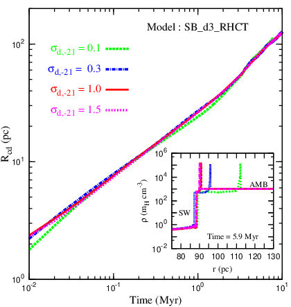
A larger $\sigma_{d}$ corresponds to a stronger radiation pressure ($P_{rad}$) at the inner layer of the shell (i.e., $f_{trap}\rightarrow 1$) but it decreases the heating efficiency because of the optical depth ($\tau$) which diminishes its strength by a factor $e^{-\tau}$. A lower value of $\sigma_{d}$ decreases the strength of $P_{rad}$ at the inner layer, but it increases heating efficiency which reflects on the shell structure.

We use the dimensionless diagnostic diagram suggested by Yeh & Matzner 2012 (hereafter YM12) to identify the dominant feedback mechanism (see Figure 1 in YM12). YM12 suggested two dimensionless parameters $\Omega$ and $\Psi$. The parameter $\Psi=R_{IF}/R_{ch}$, where $R_{IF}$ is the location of the ionized shell and $R_{ch}$ is the characteristic radius of the standard Strömgren sphere ($R_{st}$) at where the gas pressure is equal to the total unabsorbed radiation pressure $L_{bol}/(4\pi R^{2}_{st}c)$. The expression of $R_{ch}$ is given as,

where $L_{bol}$ is the bolometric luminosity and $Q_{i}$ is flux of the ionizing photons, $\mu$ and $\mu_{i}$ are the mean mass per atom and the mean mass per ion respectively, $T_{i}$ is temperature of ionized medium. Since $L_{bol}$ and $Q_{i}$ depend on the age of a cluster, the numerical value of $R_{ch}\sim 30\ L^{2}_{bol,42}\,Q^{-1}_{i,52}\,T^{-2}_{i,4}$ pc is a function of time. According to this definition, if $\Psi>1$ (i.e., $R_{ch}<R_{IF}$), the bubble expands either in standard HII regime (Strömgren sphere) or wind dominated regime, and if $\Psi<1$ then the size of the bubble is smaller than the standard case. Therefore, $\Psi$ is a measure of compactness of HII region.

The second parameter $\Omega$ is defined as

where $P_{IN}$ is the pressure at the inner edge (i.e., the edge of shell facing the driving source) of the ionized shell and $P_{IF}$ is the pressure at the ionization front (IF). Therefore, $P_{IF}V_{IF}-P_{IN}V_{IN}$ represents the difference in the product of the pressure and volume between ionization front and inner edge of the ionized shell. In our case, $R_{IN}\approx R_{cd}$ and $P_{IN}\approx P_{sw}$, and $P_{IF}$ is the pressure at outer edge of the ionized shell (i.e., $R_{edge}\approx R_{IF}$ and $P_{IF}\approx P_{edge}$), therefore $\Omega=P_{sw}R^{3}_{cd}/\left[P_{edge}R^{3}_{edge}-P_{sw}R^{3}_{cd}\right]$ (Martínez-González et al. 2014). To illustrate the significance of these parameters see Figure 11. In thin shell limit, $\Omega\approx 1/(P_{edge}/P_{sw}-1)$, where $P_{edge}$ can be simply assumed to be $P_{edge}\approx P_{sw}+P_{rad}$ and therefore, Log[$\Omega$]$<0$ represents radiation dominated regime and Log[$\Omega$]$>0$ represents wind/thermal pressure dominated regime. It is worth mentioning that, for the realistic case, $R_{edge}\neq R_{cd}$, and we find that $P_{edge}$ depends not only on the radiation pressure but also on heating and column density of the shell. Therefore, although we have seen that $\epsilon_{rad}=P_{rad}/P_{sw}$ depends weakly on the ambient density (Figure 8), here we find that $\Omega$ is density dependent (Figure 11).

The evolutionary tracks of $\Omega$ for four different $\rho_{amb}$ but for a fixed $\sigma_{d}$ are shown in Figure 12. The coloured palette on right-hand side of this figure represents the dynamical time. We see a similar evolution for different $\sigma_{d}$ (not shown in Figure 12). At early times, the size of the bubble is much smaller than $R_{ch}$ ($\approx 70$ pc) i.e., $\Psi<1$. With time the bubble size increases, and therefore, $\Psi$ keeps increasing until the first supernova. After that, $Q_{i}$ falls so rapidly that $R_{ch}$ ($\gtrsim 175$ pc) increases faster than the bubble, and $\Psi$ starts to decrease. Note that, for high density media ($\rho_{amb}\gtrsim 10^{2}$ $m{\rm{}_{H}\,cm^{-3}}$), $\Psi$ is always less than unity. This figure shows that, for high density media, the bubble moves into the radiation dominated regime (i.e., Log[$\Omega$]$<0$) from an early time ($\lesssim 0.1$ Myr). It makes transition to the thermal/wind dominated regime after $\gtrsim 3$ Myr (i.e., Log[$\Omega$]$\gtrsim 0$) which corresponds to the epoch of steep decrease in $P_{rad}/P_{sw}$ in Figure 8. For a low density medium ($\rho_{amb}\approx 1$ $m{\rm{}_{H}\,cm^{-3}}$), and bubbles always remain in the thermal pressure/wind dominated regime.

Note that, the diagnostic parameter $\Omega$ slightly overestimates the radiation dominated regime because the shell is not geometrically thin ($R_{edge}\neq R_{cd}$). In reality, the radiation pressure dominating regime ends at $\lesssim 1$ Myr (see Figure 8).

To compare with observations, we calculate the radiative output of our superbubble (model SB_d3_RHCT) at various temperatures. We create logarithmic bins in temperature ($\Delta{\rm Log}[T/K]$) and calculate the total radiative losses per unit time in each temperature bin. Figure 13 shows that radiative losses occur at molecular ($\lesssim 10^{3}$ K), nebular ($\sim 10^{4}$) and X-ray temperatures ($\sim 10^{6}-10^{8}$ K). The molecular radiation comes from the radiative relaxation layer ahead of the dense shell (see the top panel of Figure 11). The nebular emission comes from the $\sim 10^{4}$ K shell and X-rays come from the shock heated, conductively mass-loaded shocked wind. A similar temperature distribution of luminosity is seen for most of our models. The highest luminosity comes from the gas at $\sim 10^{4}$ K, which should emit in nebular lines and continuum. The luminosity in the nebular temperature band is $\sim 10^{42}$ erg sec^-1, comparable to the ionizing luminosity from driving source. A significant fraction of optical and X-ray emission is expected to be absorbed by the large column density material in the shell. In reality, the radiation leaks out because of the clumpiness in the shell. The X-ray luminosity is $\sim 10^{36-37}$ erg sec^-1, comparable to the observed X-ray luminosity of $30$ Doradus (Wang & Helfand 1991; Townsley et al. 2006).

To find the fraction of the retained input energy in superbubble, we have defined efficiency as

where $E_{IN}$ is the total amount of injected energy (i.e., work done by the radiation $E_{rad}$ and mechanical energy $E_{w}$) until a given epoch, $\Delta TE$ is the change in thermal energy (i.e., $\Delta TE=TE(t_{dyn})-TE(t_{dyn}=0)$) and $KE$ is the total kinetic energy in the simulation box at a given time (for details see Appendix C). Figure 14 displays $\eta$ as a function of dynamical time for four different ambient densities. The inset (a) shows that $\eta$ decreases monotonically as the density of the ambient medium increases, but asymptotically approaches a constant value in time. The inset (b) displays the time evolution of $\eta$ for the runs SB_d3_CT, SB_d3_HCT and SB_d3_RHCT. This figure shows that, for the runs SB_d3_HCT and SB_d3_RHCT, $\eta$ asymptotically approaches a nearly coincident value after $\gtrsim 3$ Myr (corresponds to the epoch of the first supernova; see Figure 1).

References

- Alexiades et al. (1996) Alexiades, V., Amiez, G., & Gremaud P.-A. 1996, Com. Num. Meth. Eng., 12, 31
- (2015) Bisbas, T. G., Haworth, T. J., Williams, R. J. R., Mackey, J., Tremblin, P. et al. 2015 MNRAS, 453, 1324
- (1995) Bisnovatyi-Kogan, G. S., & Silich, S. A. 1995, RvMP, 67, 661
- (1975) Castor, J., McCray, R., Weaver, R. 1975 ApJ, 200, 107
- Chevalier & Clegg (1985) Chevalier, R. A. & Clegg, A. W. 1985, Nature, 317, 44
- Cowie & McKee (1977) Cowie, L. L., & McKee, C. F. 1977, ApJ, 221, 135
- (2015) Dale, J. E. 2015, NewAR, 68, 1
- (2013) Dale, J. E., Ercolano, B., Bonnell, I. A. 2013, MNRAS, 430, 234
- (2011a) Draine, B. T. 2011a, Physics of the Interstellar and Intergalactic Medium, (Princeton University Press)
- (2011b) Draine, B. T. 2011b, ApJ, 732, 100
- (2015) Federrath, C. 2015, MNRAS, 450, 4035
- (1998) Ferland, G. J., Korista, K. T., Verner, D. A., Ferguson, J. W., Kingdon, J. B., & Verner, E. M. 1998, PASP, 110, 761
- (1993) Ferrara, A & Shchekinov, Y. 1993, ApJ, 417, 595
- (2015) Geen, S., Rosdahl, J., Blaizot, J., Devriendt, J., Slyz, A. 2015, MNRAS, 448, 3248
- (2016) Gentry, E. S., Krumholz, M. R., Dekel, A. & Madau, P. 2016, arXiv:1606.01242
- (2009) Harper-Clark, E. & Murray, N. 2009, ApJ, 693, 1696
- (2015) Haworth, T. J., Harries, T. J., Acreman, D. M., Bisbas, T. G. 2015, MNRAS, 453, 2277
- (2011) Hopkins, P. H., Quataert, E & Murray, N. 2011, MNRAS, 417, 950
- Kim et al. (2016) Kim, J., Kim, W., & Ostriker, E. C. 2016, ApJ in press, arXiv:1601.03035
- (2002) Kroupa, P., 2002, Science, 295, 82
- (2009) Krumholz, M. R., & Matzner, C. D. 2009, ApJ, 703, 1352
- Leitherer et al. (1999) Leitherer, C., Schaerer, D., Goldader, J. D., et al. 1999, ApJS, 123, 3
- Lopez et al. (2011) Lopez, L. A., Krumholz, M. R., Bolatto, A. D., Prochaska, J. X., & Ramirez-Ruiz, E. 2011, ApJ, 731, 91
- Mac Low & McCray (1988) Mac Low, M.-M., & McCray, R. 1988, ApJ, 324, 776
- Martínez-González et al. (2014) Martínez-González, S., Silich S. & Tenorio-Tagle G., 2014, ApJ, 785, 164
- (2007) Mignone, A., Bodo, G., Massaglia, S., Matsakos, T., Tesileanu, O., Zanni, C., Ferrari, A., 2007, ApJS, 170, 228
- Murray et al. (2011) Murray, N., Ménard, B. & Thompson, T. A. 2011, ApJ, 735, 66
- Parker (1965) Parker, E. N. 1965, SSRv, 4, 666
- Pellegrini et al. (2011) Pellegrini, E. W., Baldwin, J. A., & Ferland, G. J. 2011, ApJ, 738, 34
- Rogers & Pittard (2013) Rogers, H., Pittard, J. M. 2013 MNRAS, 431, 1337
- Sales et al. (2014) Sales, L. V., Marinacci, F., Springel, V., Petkova, M. 2014 MNRAS, 439, 2990
- Sharma et al. (2014) Sharma, P., Roy, A., Nath, B. B., Shchekinov, Y., 2014, MNRAS, 443, 3463
- Shu (1992) Shu, F. H., 1992, The physics of astrophysics, Volume II: Gas dynamics (University Science Books)
- Silich & Tenorio-Tagle (2013) Silich, S., Tenorio-Tagle, G., 2013, ApJ, 765, 43
- Skinner & Ostriker (2015) Skinner, M. A., & Ostriker, E. C. 2015, ApJ, 809, 187
- (1962) Spitzer, L., Jr. 1962, Physics of Fully Ionized Gases, (New York: Interscience)
- Strömgren (1939) Strömgren, B., 1939, ApJ, 89, 526
- (1950) Taylor, Geoffrey, 1950 RSPSA, 201, 159
- (1994) Toro E. F., Spruce M., Speares W., 1994, Shock Waves, 4, 25
- (2006) Townsley, L. K., Broos, P. S., Feigelson, E. D., Brandl, B. R., Chu, Y., Gamire, G. P., & Pavlov, G. G., 2006, ApJ, 131, 2140
- (1991) Wang, Q., & Helfand, D. J., 1991, ApJ, 370, 541
- (1977) Weaver, R., McCray, R., Castor, J., Shapiro, P., Moore, R., 1977, ApJ, 218, 377
- (2003) Wolfire, M. G., McKee C. F., Hollenbach, D., Tielens, A. G. G. M., 2003, ApJ, 587, 278
- Yadav et al. (2016) Yadav, N., Mukherjee, D., Sharma, P., Nath, B. B. 2016, arXiv:1603.00815v1
- (2012) Yeh, S. C. C., & Matzner, C. D. 2012, ApJ, 757, 108
Appendix A Ionization state of a gas
The state of ideal gas is mainly characterised by three variables : pressure (), density () and temperature (). At a given time, Euler equations can obtain the solutions for two of them, the third variable temperature is directly calculated from relation