跳到论文正文
W Papers独立论文阅读器 arXiv:1606.08887 论文正文 计算阅读时间 · 0%
引用这篇论文根据当前论文元数据生成,正式投稿前建议核对。


License: CC Zero
arXiv:1606.08887v1 [math.DS] 17 Jun 2016

Dynamics of the complex rational delay recursive sequence zn+1=α+β​zn−kγ−zn\displaystyle{z_{n+1}=\frac{\alpha+\beta z_{n-k}}{\gamma-z_{n}}}

Sk. Sarif Hassan Affiliation: Department of Mathematics Affiliation: University of Petroleum and Energy Studies Affiliation: Bidholi, Dehradun, India Affiliation: Email: s.hassan@ddn.upes.ac.in
Abstract

Dynamics of the delay rational difference equation zn+1=α+β​zn−kγ−zn\displaystyle{z_{n+1}=\frac{\alpha+\beta z_{n-k}}{\gamma-z_{n}}} with complex parameters α\alpha, β\beta, γ\gamma and arbitrary complex initial conditions is investigated. Existence of prime period two solutions and higher order periods are ensured in the complex parameters unlike in the case of real parameters of the same rational difference equation. In addition, a new dynamical behavior, chaotic solutions of the difference equation are ensured computationally.

Keywords: Rational difference equation, Local asymptotic stability, Chaotic trajectory and Periodicity.

Mathematics Subject Classification: 39A10 & 39A11

1 Introduction and Background

Consider the rational difference equation,

zn+1=α+β​zn−kγ−zn,n=0,1,2,…\displaystyle{z_{n+1}=\frac{\alpha+\beta z_{n-k}}{\gamma-z_{n}}},n=0,1,2,\ldots (1)

where the parameters α\alpha, β\beta, γ\gamma and the initial conditions z−k,z−k+1,…​z−1,z0z_{-k},z_{-k+1},\dots z_{-1},z_{0} are arbitrary complex numbers.

This (k+1)th order rational difference equation Eq.(1) and closely similar equations are studied when the parameters α≥0\alpha\geq 0, β>0\beta>0 and γ>0\gamma>0 and the initial conditions are real numbers while kk is any natural number [1], [2] and [3]. They have shown that the positive fixed point of Eq.(1) is a global attractor with a basin that depends on certain conditions posed on the coefficients α\alpha, β\beta and γ\gamma [1].

In this present article, an attempt has been made to study the dynamics of the rational difference equation (1) under the assumption that the parameters and the initial conditions are arbitrary complex numbers. Similar works can be found in [4], [5] and [6]. Here some of the important basics are being discussed in the following [7], [8] and [9]:

Definition 1: A difference equation of order (k+1)(k+1) is of the form

zn+1=f(zn,zn−1,…,zn−k),n=0,1,2,…\displaystyle{z_{n+1}=f(z_{n},z_{n-1},\dots,z_{n-k})},n=0,1,2,\ldots (2)

where ff is a continuous function which maps a subset 𝔻k+1\mathbb{D}^{k+1} into 𝔻\mathbb{D} and 𝔻⊂ℂ\mathbb{D}\subset\mathbb{C}. A fixed point z¯\bar{z} of the difference equation Eq. (2) is a point that satisfy the condition z¯=f⁡(z¯,z¯,…,z¯)\bar{z}=f(\bar{z},\bar{z},\dots,\bar{z}).

Definition 2: Let z¯\bar{z} be a fixed point of the Eq.(2), then z¯\bar{z} is locally asymptotically stable if for every ϵ>0\epsilon>0, there exist a δ⁡(ϵ)>0\delta(\epsilon)>0 such that, if z−k,…,z−1,z0∈z_{-k},\dots,z_{-1},z_{0}\in DD with |z−k−z¯|+⋯+|z−1−z¯|+|z0−z¯|<δ⁡(ϵ)\left\lvert z_{-k}-\bar{z}\right\rvert+\dots+\left\lvert z_{-1}-\bar{z}\right\rvert+\left\lvert z_{0}-\bar{z}\right\rvert<\delta(\epsilon), then |zn−z¯|<ϵ\left\lvert z_{n}-\bar{z}\right\rvert<\epsilon for all n≥−kn\geq-k.

Definition 3: A sequence znn=−​k∞{z_{n}}_{n=−k}^{\infty} is said to be periodic with period pp if zn+p=znz_{n+p}=z_{n} for all n≥−kn\geq-k. A sequence znn=−​k∞{z_{n}}_{n=−k}^{\infty} is said to be periodic with prime period p if pp is the smallest positive integer having this property.

Definition 4: An open ball B⁡(a,r)∈ℂB(a,r)\in\mathbb{C} is called an invariant open ball of Eq.(2) if z−k,…,z−1,z0∈B⁡(a,r)z_{-k},\dots,z_{-1},z_{0}\in B(a,r) then zn∈B⁡(a,r)z_{n}\in B(a,r) for all n>0n>0. That is every solution of Eq.(2) with initial conditions in B⁡(a,r)B(a,r) remains in B⁡(a,r)B(a,r).

Definition 5: The difference equation Eq.(2) is said to be permanent and bounded if there exist positive real numbers MM and NN with 0<M≤N<∞0<M\leq N<\infty such that for any initial conditions z−k,…,z−1,z0z_{-k},\dots,z_{-1},z_{0} there exist a positive integer P which depends on the initial conditions such that M≤|zn|≤NM\leq\left\lvert z_{n}\right\rvert\leq N for all n≥Pn\geq P.

The linearized equation associated with Eq.(2) about the equilibrium point z¯\bar{z} is

yn+1=∑i=0k∂f⁡(z¯,z¯,…,z¯)∂ui​yn−iy_{n+1}=\sum_{i=0}^{k}\frac{\partial f(\bar{z},\bar{z},\dots,\bar{z})}{\partial u_{i}}y_{n-i}

Its characteristic equation is

λk+1=∑i=0k∂f⁡(z¯,z¯,…,z¯)∂ui​λn−i\lambda^{k+1}=\sum_{i=0}^{k}\frac{\partial f(\bar{z},\bar{z},\dots,\bar{z})}{\partial u_{i}}\lambda^{n-i}

where n=0,1,2,…n=0,1,2,\dots.

Theorem 1.1.

Assume that ff is a C1C^{1}-function and let z¯\bar{z} a fixed point of Eq.(2). Then the following statements are true:

  • •

    If all the roots of the characteristic equation lie in the open unit disk |λ|<1\left\lvert\lambda\right\rvert<1, then the fixed point z¯\bar{z} of Eq.(2) is locally asymptotically stable.

  • •

    If at least one root of the characteristic equation has the absolute value greater than one, then the fixed point z¯\bar{z} of Eq.(2) is unstable.

  • •

    If all the roots of the have the characteristic equation absolute value greater than one, then the fixed point z¯\bar{z} of Eq.(2) is a source.

Theorem 1.2.

Assume that pp, qq ∈ℂ\in\mathbb{C} and k∈ℕk\in\mathbb{N}. Then |p|+|q|<1\left\lvert p\right\rvert+\left\lvert q\right\rvert<1 is a sufficient condition for asymptotically stability of the difference equation

zn+1−pzn+qzn−k=0,n=0,1,2,3,…z_{n+1}-pz_{n}+qz_{n-k}=0,n=0,1,2,3,\dots

Now we shall use these basic theorems to explore the local stability of the fixed points of the Eq.(1).

2 Local Asymptotic Stability of the Fixed Points and Boundedness

The fixed points of Eq.(1) are the solutions of the quadratic equation

z¯=α+β​z¯γ−z¯\bar{z}=\frac{\alpha+\beta\bar{z}}{\gamma-\bar{z}}

Eq.(1) has the two fixed points z¯1\bar{z}_{1} and z¯2\bar{z}_{2} when |α|≠|(γ−β)24|\left\lvert\alpha\right\rvert\neq\left\lvert\frac{({\gamma-\beta})^{2}}{4}\right\rvert …
12​(−−4​α+β2−2​β​γ+γ2−β+γ)\frac{1}{2}\left(-\sqrt{-4\alpha+\beta^{2}-2\beta\gamma+\gamma^{2}}-\beta+\gamma\right) and 12​(−4​α+β2−2​β​γ+γ2−β+γ)\frac{1}{2}\left(\sqrt{-4\alpha+\beta^{2}-2\beta\gamma+\gamma^{2}}-\beta+\gamma\right) respectively.

It is noted that if α=(γ−β)24\alpha=\frac{({\gamma-\beta})^{2}}{4}, then there is only one fixed point, (γ−β)2\frac{(\gamma-\beta)}{2}.

The linearized equation of the rational difference equation Eq.(1) with respect to the fixed points z¯\bar{z} is

zn+1−α+β​z¯(γ−z¯)2zn−βγ−z¯zn−k=0,n=0,1,…\displaystyle{z_{n+1}-\frac{\alpha+\beta\bar{z}}{(\gamma-\bar{z})^{2}}z_{n}-\frac{\beta}{\gamma-\bar{z}}z_{n-k}=0,n=0,1,\ldots} (3)

with associated characteristic equation

λk+1−α+β​z¯(γ−z¯)2​λk−βγ−z¯=0.\lambda^{k+1}-\frac{\alpha+\beta\bar{z}}{(\gamma-\bar{z})^{2}}\lambda^{k}-\frac{\beta}{\gamma-\bar{z}}=0.\\ (4)

The linearized equation for the fixed point (γ−β)2\frac{(\gamma-\beta)}{2} is

zn+1−γ−βγ+βzn−2​ββ+γzn−k=0,n=0,1,…\displaystyle{z_{n+1}-\frac{\gamma-\beta}{\gamma+\beta}z_{n}-\frac{2\beta}{\beta+\gamma}z_{n-k}=0,n=0,1,\ldots} (5)

with associated characteristic equation

λk+1−γ−βγ+β​λk−2​ββ+γ=0.\lambda^{k+1}-\frac{\gamma-\beta}{\gamma+\beta}\lambda^{k}-\frac{2\beta}{\beta+\gamma}=0. (6)

It is found that there does not exist any α\alpha, β\beta and γ\gamma in ℂ\mathbb{C} such that α=(γ−β)24\alpha=\frac{({\gamma-\beta})^{2}}{4} in 𝔻∈ℂ\mathbb{D}\in\mathbb{C} for which the condition

|γ−βγ+β|+|2​ββ+γ|<1\left\lvert\frac{\gamma-\beta}{\gamma+\beta}\right\rvert+\left\lvert\frac{2\beta}{\beta+\gamma}\right\rvert<1

Hence the fixed point (γ−β)2\frac{(\gamma-\beta)}{2} is not locally asymptotically stable.

The following result gives the local asymptotic stability of the fixed point …
12​(−−4​α+β2−2​β​γ+γ2−β+γ)\frac{1}{2}\left(-\sqrt{-4\alpha+\beta^{2}-2\beta\gamma+\gamma^{2}}-\beta+\gamma\right) and 12​(−4​α+β2−2​β​γ+γ2−β+γ)\frac{1}{2}\left(\sqrt{-4\alpha+\beta^{2}-2\beta\gamma+\gamma^{2}}-\beta+\gamma\right) of the Eq.(1).

Theorem 2.1.

The fixed point 12​(−−4​α+β2−2​β​γ+γ2−β+γ)\frac{1}{2}\left(-\sqrt{-4\alpha+\beta^{2}-2\beta\gamma+\gamma^{2}}-\beta+\gamma\right) of Eq.(1) is locally asymptotically stable if

|2​β(β−γ)2−4​α+β+γ|+|γ⁡(−(β−γ)2−4​α−β+γ)−2​α2​(α+β​γ)|<1\left\lvert\frac{2\beta}{\sqrt{(\beta-\gamma)^{2}-4\alpha}+\beta+\gamma}\right\rvert+\left\lvert\frac{\gamma\left(-\sqrt{(\beta-\gamma)^{2}-4\alpha}-\beta+\gamma\right)-2\alpha}{2(\alpha+\beta\gamma)}\right\rvert<1
Theorem 2.2.

The fixed point 12​(−4​α+β2−2​β​γ+γ2−β+γ)\frac{1}{2}\left(\sqrt{-4\alpha+\beta^{2}-2\beta\gamma+\gamma^{2}}-\beta+\gamma\right) of Eq.(1) is locally asymptotically stable if

|2​β−(β−γ)2−4​α+β+γ|+|γ⁡((β−γ)2−4​α−β+γ)−2​α2​(α+β​γ)|<1\left\lvert\frac{2\beta}{-\sqrt{(\beta-\gamma)^{2}-4\alpha}+\beta+\gamma}\right\rvert+\left\lvert\frac{\gamma\left(\sqrt{(\beta-\gamma)^{2}-4\alpha}-\beta+\gamma\right)-2\alpha}{2(\alpha+\beta\gamma)}\right\rvert<1

Proof of these two theorems are straightforward from the result stated in the Theorem 1.2. Here we go with few examples which illustrate the asymptotic behavior of these two fixed points.

S.n. Parameters α\alpha, β\beta, γ\gamma Remark
1 α→−107.7−374.6​i,β→56−91.2​i,γ→147.4+210​i\alpha\to-107.7-374.6i,\beta\to 56-91.2i,\gamma\to 147.4+210i Here modulus of the zeros of the characteristic equation are both less than one and so the fixed point is locally asymptotically stable. It is found that for all k=1,2,3,…k=1,2,3,\dots, The trajectories are convergent to the fixed point 12​(−−4​α+β2−2​β​γ+γ2−β+γ)\frac{1}{2}\left(-\sqrt{-4\alpha+\beta^{2}-2\beta\gamma+\gamma^{2}}-\beta+\gamma\right).
2 α→−297.4−75.3​i,β→78−71.6​i,γ→−220.6−128.5​i\alpha\to-297.4-75.3i,\beta\to 78-71.6i,\gamma\to-220.6-128.5i Here modulus of the zeros of the characteristic equation are less than one and so the fixed point 12​(−4​α+β2−2​β​γ+γ2−β+γ)\frac{1}{2}\left(\sqrt{-4\alpha+\beta^{2}-2\beta\gamma+\gamma^{2}}-\beta+\gamma\right) is locally asymptotically stable. It is found that for all k=1,2,3,…k=1,2,3,\dots, The trajectories are convergent to the fixed point.
Table 1: Parameters α\alpha, β\beta and γ\gamma for which the fixed points 12​(±−4​α+β2−2​β​γ+γ2−β+γ)\frac{1}{2}\left(\pm\sqrt{-4\alpha+\beta^{2}-2\beta\gamma+\gamma^{2}}-\beta+\gamma\right) of Eq.(1) are locally asymptotically stable for arbitrary initial values.
Refer to caption Refer to caption
Figure 1: Local Asymptotical Stability of the fixed points. In the top of the figure, for different values of kk, complex trajectories plot (left) and their corresponding time series plot with real and imaginary part (right) are given for the fixed point 12​(−−4​α+β2−2​β​γ+γ2−β+γ)\frac{1}{2}\left(-\sqrt{-4\alpha+\beta^{2}-2\beta\gamma+\gamma^{2}}-\beta+\gamma\right). Same is given in the bottom for the other fixed point.

In the Table-1 as stated, for the parameters given in the serial number 11 and 22, the trajectories are convergent and converge to the fixed points 12​(−−4​α+β2−2​β​γ+γ2−β+γ)\frac{1}{2}\left(-\sqrt{-4\alpha+\beta^{2}-2\beta\gamma+\gamma^{2}}-\beta+\gamma\right) and 12​(−4​α+β2−2​β​γ+γ2−β+γ)\frac{1}{2}\left(\sqrt{-4\alpha+\beta^{2}-2\beta\gamma+\gamma^{2}}-\beta+\gamma\right) of Eq.(1) respectively for all delay term kk.

Further, a matrix of 2020 rows of parameters α\alpha, β\beta and γ\gamma for which the fixed point 12​(−−4​α+β2−2​β​γ+γ2−β+γ)\frac{1}{2}\left(-\sqrt{-4\alpha+\beta^{2}-2\beta\gamma+\gamma^{2}}-\beta+\gamma\right) of Eq.(1) is locally asymptotically stable, is given here. In each row the first, second and third complex number referred as α\alpha, β\beta and γ\gamma respectively.

(2213.8−627.2​i−1158.7−591.8​i4355.−33.7​i−1755.8−435.3​i1657.2−99.3​i3223.4−1018.8​i−880.8+1780.7​i−1282.1−813.5​i−555.−3870.8​i2860.1+1430​i−1262.7−860​i−643.8+3893.9​i−2501.1+1648.8​i1508.5+1652.8​i1773.1−4323.1​i−60.8−492​i7.9−90.7​i307.5+659​i2750.5−1175.1​i−953.7+392.9​i3987.6+1450.2​i338.9+77.1​i−203.4−84.8​i750.7+226.7​i−635.5+187.8​i−224.9−840.4​i1347.8+1812.5​i18+69.1​i1.2+45.3​i276.5−26.2​i1055.8+3679.6​i501.5−369.8​i1400.3+1747.7​i2337.3+4233.9​i−377.3−451.5​i120.7+1373.2​i3231.5+700.7​i−968.6−1000.5​i3070.4−968.5​i2021.8+1066.1​i−361.+739​i3616.2+1451.6​i−1058.1+1749.3​i357.7+4.8​i788.9−3083.i−890.5+1361.9​i−1421.6−670.8​i116.4−3391.3​i−3635.7−4440.8​i−1692.9+1093​i3719.2−3308.7​i−76.2+2700.8​i−733.+1500​i3174.1+1390​i−1883.8−4906.7​i−1490.2+742.2​i2899.5−4163.9​i301+1028.6​i−112.9−1099.1​i2190.1−3783.9​i)\left(\begin{array}[]{ccc}2213.8\,-627.2i&-1158.7-591.8i&4355.\,-33.7i\\ -1755.8-435.3i&1657.2\,-99.3i&3223.4\,-1018.8i\\ -880.8+1780.7i&-1282.1-813.5i&-555.-3870.8i\\ 2860.1\,+1430i&-1262.7-860i&-643.8+3893.9i\\ -2501.1+1648.8i&1508.5\,+1652.8i&1773.1\,-4323.1i\\ -60.8-492i&7.9\,-90.7i&307.5\,+659i\\ 2750.5\,-1175.1i&-953.7+392.9i&3987.6\,+1450.2i\\ 338.9\,+77.1i&-203.4-84.8i&750.7\,+226.7i\\ -635.5+187.8i&-224.9-840.4i&1347.8\,+1812.5i\\ 18\,+69.1i&1.2\,+45.3i&276.5\,-26.2i\\ 1055.8\,+3679.6i&501.5\,-369.8i&1400.3\,+1747.7i\\ 2337.3\,+4233.9i&-377.3-451.5i&120.7\,+1373.2i\\ 3231.5\,+700.7i&-968.6-1000.5i&3070.4\,-968.5i\\ 2021.8\,+1066.1i&-361.+739i&3616.2\,+1451.6i\\ -1058.1+1749.3i&357.7\,+4.8i&788.9\,-3083.i\\ -890.5+1361.9i&-1421.6-670.8i&116.4\,-3391.3i\\ -3635.7-4440.8i&-1692.9+1093i&3719.2\,-3308.7i\\ -76.2+2700.8i&-733.+1500i&3174.1\,+1390i\\ -1883.8-4906.7i&-1490.2+742.2i&2899.5\,-4163.9i\\ 301\,+1028.6i&-112.9-1099.1i&2190.1\,-3783.9i\\ \end{array}\right)

Similarly, the fixed point 12​(−4​α+β2−2​β​γ+γ2−β+γ)\frac{1}{2}\left(\sqrt{-4\alpha+\beta^{2}-2\beta\gamma+\gamma^{2}}-\beta+\gamma\right) of Eq.(1) is locally asymptotically stable for the set of parameters which is given as matrix as follows:

(2686.1−1250.3​i629.7−417​i−1594.+4310.2​i1419.2−2938.1​i588.9−568.9​i−2005.2+421​i763.8+3108​i−646.−533.3​i−1073.2−3104.1​i2816.4−1018.7​i−503.9−401.1​i−2364.7−2712.i−106.2−138.8​i231.4+106.1​i−631.5+854.9​i2608.3−3767.4​i−363.6−366.9​i−1909.8+299.2​i3435.3+2539.7​i535.3+20.1​i−618.1+2127.1​i−984.2+955.5​i666.8−431.4​i26.−2208.2​i−2113.7+3096.8​i991.3+434.3​i−326.8−3814.8​i−669.8−794.3​i−86.8−1545.9​i−3677.5+1627.6​i2663.8−2211​i1366.2+1397.7​i−3862.−2238.9​i575+221​i1515.2−8.2​i1087.6+4131.8​i992.7−772​i180.9−1155.2​i−2175.5−885.1​i3337.7+2555​i−1931.1+111.4​i−2914.1−4788​i982.5+492.9​i807.6+666.8​i−3412.6−1495.6​i1908.8+3639.9​i−527.4+1553.7​i−3264.5+645.1​i1393.1−853.1​i261.1+1276.7​i−2089.8−4087.5​i−1931.3−1221.9​i340.2−527.6​i−1151.6−2448​i−1319.1+724.3​i394.1+798.2​i−4187.5−992.1​i1582.8+350.7​i251.5+37.2​i−2431.8+892.6​i)\left(\begin{array}[]{ccc}2686.1\,-1250.3i&629.7\,-417i&-1594.+4310.2i\\ 1419.2\,-2938.1i&588.9\,-568.9i&-2005.2+421i\\ 763.8\,+3108i&-646.-533.3i&-1073.2-3104.1i\\ 2816.4\,-1018.7i&-503.9-401.1i&-2364.7-2712.i\\ -106.2-138.8i&231.4\,+106.1i&-631.5+854.9i\\ 2608.3\,-3767.4i&-363.6-366.9i&-1909.8+299.2i\\ 3435.3\,+2539.7i&535.3\,+20.1i&-618.1+2127.1i\\ -984.2+955.5i&666.8\,-431.4i&26.\,-2208.2i\\ -2113.7+3096.8i&991.3\,+434.3i&-326.8-3814.8i\\ -669.8-794.3i&-86.8-1545.9i&-3677.5+1627.6i\\ 2663.8\,-2211i&1366.2\,+1397.7i&-3862.-2238.9i\\ 575\,+221i&1515.2\,-8.2i&1087.6\,+4131.8i\\ 992.7\,-772i&180.9\,-1155.2i&-2175.5-885.1i\\ 3337.7\,+2555i&-1931.1+111.4i&-2914.1-4788i\\ 982.5\,+492.9i&807.6\,+666.8i&-3412.6-1495.6i\\ 1908.8\,+3639.9i&-527.4+1553.7i&-3264.5+645.1i\\ 1393.1\,-853.1i&261.1\,+1276.7i&-2089.8-4087.5i\\ -1931.3-1221.9i&340.2\,-527.6i&-1151.6-2448i\\ -1319.1+724.3i&394.1\,+798.2i&-4187.5-992.1i\\ 1582.8\,+350.7i&251.5\,+37.2i&-2431.8+892.6i\\ \end{array}\right)

The 100100 set of such parameters α\alpha, β\beta and γ\gamma are plotted in the complex plane in the following Fig. 2.

Refer to caption
Refer to caption
Figure 2: Parameters α\alpha, β\beta and γ\gamma plot for which the fixed points are locally asymptotically stable. Here the top figure stands for the fixed point 12​(−4​α+β2−2​β​γ+γ2−β+γ)\frac{1}{2}\left(\sqrt{-4\alpha+\beta^{2}-2\beta\gamma+\gamma^{2}}-\beta+\gamma\right) and bottom one stands for the fixed point 12​(−4​α+β2−2​β​γ+γ2−β+γ)\frac{1}{2}\left(\sqrt{-4\alpha+\beta^{2}-2\beta\gamma+\gamma^{2}}-\beta+\gamma\right).

2.1 Local Asymptotic Stability in the case α=0,∈ℂ\alpha=0,\in\mathbb{C}

When the parameter α=0\alpha=0, then the the difference equation Eq.(1) would reduce to

zn+1=β​zn−kγ−zn,n=0,1,…,k∈1,2,…\displaystyle{z_{n+1}=\frac{\beta z_{n-k}}{\gamma-z_{n}},n=0,1,\ldots,k\in{1,2,\dots}} (7)

The fixed points z±z_{\pm} of the equation Eq.(7) are 00 and γ−β\gamma-\beta respectively.

In the similar fashion we did earlier, the fixed point z+=0z_{+}=0 of the difference equation Eq.(7) is locally asymptotically stable, unstable if |βγ|<1\left\lvert\frac{\beta}{\gamma}\right\rvert<1, |βγ|>1\left\lvert\frac{\beta}{\gamma}\right\rvert>1 respectively.

Similarly, the fixed point z−=γ−βz_{-}=\gamma-\beta is locally asymptotically stable if |γβ−1|<0\left\lvert\frac{\gamma}{\beta}-1\right\rvert<0 i.e. |γβ|<1\left\lvert\frac{\gamma}{\beta}\right\rvert<1. If |γβ|>1\left\lvert\frac{\gamma}{\beta}\right\rvert>1 then the fixed point is unstable.

2.2 Local Asymptotic Stability in the case α=β=γ\alpha=\beta=\gamma

When all the three parameters are same (β=γ=α)(\beta=\gamma=\alpha), then the difference equation Eq.(1) becomes

zn+1=α+α​zn−kα−zn,n=0,1,2,…\displaystyle{z_{n+1}=\frac{\alpha+\alpha z_{n-k}}{\alpha-z_{n}}},n=0,1,2,\ldots (8)

The fixed points of the difference equation Eq.(8) are ±i​α\pm i\sqrt{\alpha}.

The fixed points ±i​α\pm i\sqrt{\alpha} of Eq.(8) are locally asymptotically stable if

|21+∓iα|<1\left\lvert\frac{2}{1+\mp\frac{i}{\sqrt{\alpha}}}\right\rvert<1

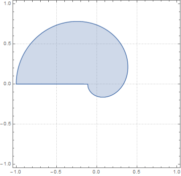
Here we shall look for the subset 𝕊\mathbb{S} of ℂ\mathbb{C} of the parameter α\alpha for which the above stated condition does hold good. Before seeking the set of our interest, let us try to envisage the region and we found it to be the following in the Fig. 3 where the real part and imaginary part of the parameter α\alpha are assumed to varied over the region (−1,1)×(−1,1)(-1,1)\times(-1,1).

Now we can see what we are to find, i.e. dependence of the boundary of this set, i.e. we should find a few functions yielding yy as a function of xx on the boundary. where α=x+i​y\alpha=x+iy. We have the following xx and yy which satisfy the boundary |21+∓iα|=1\left\lvert\frac{2}{1+\mp\frac{i}{\sqrt{\alpha}}}\right\rvert=1.

[Uncaptioned image]
Refer to caption
Figure 3: Region of the parameter α\alpha while its real and imaginary part are varying along the (-1,1) and (-1,1) respectively.

To figure out why the solution looks slightly involved, we plot all the roots of the underlying polynomial then the curves will form more symmetric pattern:

Refer to caption
Figure 4: Boundary of the roots of the underlying polynomials. Different colors denote four different polynomials.

Here we go with a set of examples of parameter α\alpha for which the fixed points ±i​α\pm i\sqrt{\alpha} of the difference equation Eq.(8) are locally asymptotically stable.

A={{α→0.294548+0.27933i},{α→0.303387i},{α→−0.111111},{α→−0.111111+0.288786i},{α→−0.12042i}}\{\{\alpha\to 0.294548\,+0.27933i\},\{\alpha\to 0.303387i\},\{\alpha\to-0.111111\},\{\alpha\to-0.111111+0.288786i\},\{\alpha\to-0.12042i\}\}

B={{α→−0.428571i},{α→−0.526596−0.0285714i},{α→−0.0725055},{α→0.325133−0.0233645i},{α→0.28391+0.0116959i}}\{\{\alpha\to-0.428571i\},\{\alpha\to-0.526596-0.0285714i\},\{\alpha\to-0.0725055\},\{\alpha\to 0.325133\,-0.0233645i\},\{\alpha\to 0.28391\,+0.0116959i\}\}

For these two sets A and B of parameters the fixed points ∓i​α\mp i\sqrt{\alpha} is locally asymptotically stable respectively.

2.3 Permanence and Boundedness of Solutions

Theorem 2.3.

Let |α|<|(γ−β)24|\left\lvert\alpha\right\rvert<\left\lvert\frac{(\gamma-\beta)^{2}}{4}\right\rvert and the initial values z−k,z−k+1,…,z−1,z0∈B⁡(0,|z¯1|)z_{-k},z_{-k+1},\dots,z_{-1},z_{0}\in B(0,\left\lvert\bar{z}_{1}\right\rvert). If {zn}\{z_{n}\} is any solution of Eq.(1), then zn∈B⁡(0,|z¯1|)z_{n}\in B(0,\left\lvert\bar{z}_{1}\right\rvert) for all n≥1n\geq 1, that is {zn}\{z_{n}\} is permanent and bounded.

Proof: If the the initial values z−k,z−k+1,…,z−1,z0∈B⁡(0,|z¯1|)z_{-k},z_{-k+1},\dots,z_{-1},z_{0}\in B(0,\left\lvert\bar{z}_{1}\right\rvert), then |z−k|<|z¯1|,|z−k+1|<|z¯1|,…,|z−1|<|z¯1|\left\lvert z_{-k}\right\rvert<\left\lvert\bar{z}_{1}\right\rvert,\left\lvert z_{-k+1}\right\rvert<\left\lvert\bar{z}_{1}\right\rvert,\dots,\left\lvert z_{-1}\right\rvert<\left\lvert\bar{z}_{1}\right\rvert and |z0|<|z¯1|\left\lvert z_{0}\right\rvert<\left\lvert\bar{z}_{1}\right\rvert, we have

0<|z1|=|α+β​z−kγ−z0|<|α+β​z¯1γ−z¯1|=|z¯1|0<\left\lvert z_{1}\right\rvert=\left\lvert\frac{\alpha+\beta z_{-k}}{\gamma-z_{0}}\right\rvert<\left\lvert\frac{\alpha+\beta\bar{z}_{1}}{\gamma-\bar{z}_{1}}\right\rvert=\left\lvert\bar{z}_{1}\right\rvert

Similarly,

0<|z2|=|α+β​z−k+1γ−z1|<|α+β​z¯1γ−z¯1|=|z¯1|0<\left\lvert z_{2}\right\rvert=\left\lvert\frac{\alpha+\beta z_{-k+1}}{\gamma-z_{1}}\right\rvert<\left\lvert\frac{\alpha+\beta\bar{z}_{1}}{\gamma-\bar{z}_{1}}\right\rvert=\left\lvert\bar{z}_{1}\right\rvert

Using Mathematical Induction we have 0<|zn|<|z¯1|0<\left\lvert z_{n}\right\rvert<\left\lvert\bar{z}_{1}\right\rvert for all n≥1n\geq 1. Therefore, the open ball B⁡(0,|z¯1|)B(0,\left\lvert\bar{z}_{1}\right\rvert) is invariant of Eq.(1) and the solution {zn}\{z_{n}\} of Eq.(1) is permanent and bounded.

Theorem 2.4.

Let |α|=|(γ−β)24|\left\lvert\alpha\right\rvert=\left\lvert\frac{(\gamma-\beta)^{2}}{4}\right\rvert and the initial values z−k,z−k+1,…,z−1,z0∈B⁡(0,|γ−β2|)z_{-k},z_{-k+1},\dots,z_{-1},z_{0}\in B(0,\left\lvert\frac{\gamma-\beta}{2}\right\rvert) where |β|<|3​γ|\left\lvert\beta\right\rvert<\left\lvert 3\gamma\right\rvert. If {zn}\{z_{n}\} is any solution of Eq.(1), then zn∈B⁡(0,|γ−β2|)z_{n}\in B(0,\left\lvert\frac{\gamma-\beta}{2}\right\rvert) for all n≥1n\geq 1, that is {zn}\{z_{n}\} is permanent and bounded.

Proof: Considering |β|<|3​γ|\left\lvert\beta\right\rvert<\left\lvert 3\gamma\right\rvert, we have 0<|γ−β2|<|γ|0<\left\lvert\frac{\gamma-\beta}{2}\right\rvert<\left\lvert\gamma\right\rvert and the initial values z−k,z−k+1,…,z−1,z0∈B⁡(0,|γ−β2|)z_{-k},z_{-k+1},\dots,z_{-1},z_{0}\in B(0,\left\lvert\frac{\gamma-\beta}{2}\right\rvert), then |z−k|<|γ−β2|,|z−k+1|<|γ−β2|,…,|z−1|<|γ−β2|\left\lvert z_{-k}\right\rvert<\left\lvert\frac{\gamma-\beta}{2}\right\rvert,\left\lvert z_{-k+1}\right\rvert<\left\lvert\frac{\gamma-\beta}{2}\right\rvert,\dots,\left\lvert z_{-1}\right\rvert<\left\lvert\frac{\gamma-\beta}{2}\right\rvert and |z0|<|γ−β2|\left\lvert z_{0}\right\rvert<\left\lvert\frac{\gamma-\beta}{2}\right\rvert, we have

0<|z1|=|α+β​z−kγ−z0|<|α+β​γ−β2γ−γ−β2|=|γ−β2|0<\left\lvert z_{1}\right\rvert=\left\lvert\frac{\alpha+\beta z_{-k}}{\gamma-z_{0}}\right\rvert<\left\lvert\frac{\alpha+\beta\frac{\gamma-\beta}{2}}{\gamma-\frac{\gamma-\beta}{2}}\right\rvert=\left\lvert\frac{\gamma-\beta}{2}\right\rvert

Similarly,

0<|z2|=|α+β​z−k+1γ−z1|<|α+β​γ−β2γ−γ−β2|=|γ−β2|0<\left\lvert z_{2}\right\rvert=\left\lvert\frac{\alpha+\beta z_{-k+1}}{\gamma-z_{1}}\right\rvert<\left\lvert\frac{\alpha+\beta\frac{\gamma-\beta}{2}}{\gamma-\frac{\gamma-\beta}{2}}\right\rvert=\left\lvert\frac{\gamma-\beta}{2}\right\rvert

Using Mathematical Induction we have 0<|zn|<|γ−β2|0<\left\lvert z_{n}\right\rvert<\left\lvert\frac{\gamma-\beta}{2}\right\rvert for all n≥1n\geq 1. Therefore, the open ball B⁡(0,|γ−β2|)B(0,\left\lvert\frac{\gamma-\beta}{2}\right\rvert) is invariant of Eq.(1) and the solution {zn}\{z_{n}\} of Eq.(1) is permanent and bounded.

An example is taken here as an evidence of the Theorem 2.4. Consider γ=5+6​i\gamma=5+6i, β=2+3​i\beta=2+3i and so α=|(γ−β)24|=0+4.5​i\alpha=\left\lvert\frac{(\gamma-\beta)^{2}}{4}\right\rvert=0+4.5i. Here the fixed point is γ−β2=1.5+1.5​i\frac{\gamma-\beta}{2}=1.5+1.5i with modulus 2.12132.1213. Also we assume k=2 and the initial values z−2=i,z−1=1+iz_{-2}=i,z_{-1}=1+i and z0=1.5+iz_{0}=1.5+i note that |z−2|,|z−1|\left\lvert z_{-2}\right\rvert,\left\lvert z_{-1}\right\rvert and |z0|\left\lvert z_{0}\right\rvert are all less than |γ−β2|=2.1213\left\lvert\frac{\gamma-\beta}{2}\right\rvert=2.1213 and |β|<3​|γ|\left\lvert\beta\right\rvert<3\left\lvert\gamma\right\rvert. So the Theorem 2.4 is applicable here. What we expect is that all the solution {zn}\{z_{n}\} of Eq.(1) is permanent and bounded, that is 0<|zn|<|γ−β2|0<\left\lvert z_{n}\right\rvert<\left\lvert\frac{\gamma-\beta}{2}\right\rvert for all n≥1n\geq 1. The complex trajectory plot including its time series plot are given in the Fig. 5.

Refer to caption Refer to caption
Figure 5: Complex trajectory plot including its time series plot.

In the Fig. 55, it is seen that all the solutions {zn}\{z_{n}\} of Eq.(1) are lying in the disk B⁡(0,|γ−β2|)B(0,\left\lvert\frac{\gamma-\beta}{2}\right\rvert).

3 Periodic of Solutions

We shall first look for the prime period two solutions of the three difference equation Eq.(1).

Let …,ϕ,ψ,ϕ,ψ,…\ldots,\phi,~\psi,~\phi,~\psi,\ldots, ϕ≠ψ\phi\neq\psi be a prime period two solution of the difference equation Eq.(1).
If kk is even, then zn=zn−kz_{n}=z_{n-k} and then ψ=α+β​ϕγ−ϕ\psi=\frac{\alpha+\beta\phi}{\gamma-\phi} and ϕ=α+β​ψγ−ψ\phi=\frac{\alpha+\beta\psi}{\gamma-\psi}. By solving these two equations we get (γ+β)​(ψ−ϕ)=0(\gamma+\beta)(\psi-\phi)=0. So γ=−β\gamma=-\beta will lead to prime period two solutions of the difference equation Eq.(1).
if kk is odd, then zn+1=zn−kz_{n+1}=z_{n-k} and then ψ=α+β​ψγ−ϕ\psi=\frac{\alpha+\beta\psi}{\gamma-\phi} and ϕ=α+β​ϕγ−ψ\phi=\frac{\alpha+\beta\phi}{\gamma-\psi}. By solving these two equations we get (γ−β)​(ψ−ϕ)=0(\gamma-\beta)(\psi-\phi)=0. Therefore γ=β\gamma=\beta will lead to prime period two solutions of the difference equation Eq.(1).

It is noted that for γ>β>0\gamma>\beta>0 in the real line, there was no prime period two solution of the difference equation Eq.(1). Here we list a few examples where we found the higher order periods viz. 9,10,139,10,13 and etc.

Parameters: α\alpha, β\beta, γ\gamma and Delay term: kk Periodic Solutions Remarks
α=0.2729+0.0372​i\alpha=0.2729+0.0372i, β=0.7690+0.3960​i\beta=0.7690+0.3960i, γ=−β\gamma=-\beta and k=1k=1 ψ=−0.0444+0.1575​i\psi=-0.0444+0.1575i ϕ=0.2333+1.6669​i\phi=0.2333+1.6669i, Period: 2 [Uncaptioned image]
α=0.4024+0.9828​i\alpha=0.4024+0.9828i, β=0.0740+0.6841​i\beta=0.0740+0.6841i, γ=β\gamma=\beta and k=2k=2 ψ=−0.5589−0.1317​i\psi=-0.5589-0.1317i ϕ=−0.1991+0.9915​i\phi=-0.1991+0.9915i, Period: 2 [Uncaptioned image]
α=−0.1111+0.2337​i\alpha=-0.1111+0.2337i, β=α\beta=\alpha, γ=β\gamma=\beta and k=6k=6 Period: 9 [Uncaptioned image]
α=−0.1111+0.2337​i\alpha=-0.1111+0.2337i, β=α\beta=\alpha, γ=β\gamma=\beta and k=8k=8 Period: 11 [Uncaptioned image]
α=−0.1111+0.2337​i\alpha=-0.1111+0.2337i, β=α\beta=\alpha, γ=β\gamma=\beta and k=12k=12 Period: 15 [Uncaptioned image]
α=−0.1111+0.2337​i\alpha=-0.1111+0.2337i, β=α\beta=\alpha, γ=β\gamma=\beta and k=17k=17 Period: 20 [Uncaptioned image]
Table 2: Higher Order Periodic Solutions where γ=±β\gamma=\pm\beta, of the equation Eq.(1) for different initial values. In the right most column the corresponding periodic trajectory plots are given.
Parameters: α\alpha, β\beta, γ\gamma and Delay term: kk Periodic Solutions Remarks
α=−0.1111+0.2337​i\alpha=-0.1111+0.2337i, β=α\beta=\alpha, γ=β\gamma=\beta and k=38k=38 Period: 41 [Uncaptioned image]
α=−0.1111+0.2337​i\alpha=-0.1111+0.2337i, β=α\beta=\alpha, γ=β\gamma=\beta and k=40k=40 Period: 43 [Uncaptioned image]
α=−0.1111+0.2337​i\alpha=-0.1111+0.2337i, β=α\beta=\alpha, γ=β\gamma=\beta and k=52k=52 Period: 55 [Uncaptioned image]
α=−0.1111+0.2337​i\alpha=-0.1111+0.2337i, β=α\beta=\alpha, γ=β\gamma=\beta and k=80k=80 Period: 83 [Uncaptioned image]
α=−0.1111+0.2337​i\alpha=-0.1111+0.2337i, β=α\beta=\alpha, γ=β\gamma=\beta and k=100k=100 Period: 103 [Uncaptioned image]
α=−0.1111+0.2337​i\alpha=-0.1111+0.2337i, β=α\beta=\alpha, γ=β\gamma=\beta and k=5100k=5100 Period: 5103 [Uncaptioned image]
Table 3: Higher Order Periodic Solutions where γ=±β\gamma=\pm\beta, of the equation Eq.(1) for different initial values. In the right most column the corresponding periodic trajectory plots are given.

In the Table 22 and Table 33, a set of examples of higher order periods are given for different values of kk and parameters. What is interesting to note here is that the period is associated to the delay term kk as p=k+3p=k+3 (pp denotes period) where all the parameters are taken as same (α=β=γ\alpha=\beta=\gamma). This inspired us to propose the following conjectures.

Conjecture 3.1.

There exist as many as higher order periods of the difference Eq.(1) is demanded.

Conjecture 3.2.

For α=β=γ\alpha=\beta=\gamma, period (pp) is increased by 33 with the delay term kk. i.e. p=k+3p=k+3.

4 Chaotic Solutions

A new dynamical behavior of the rational difference equation Eq.(1) is chaoticity which was not present in the real set of parameters. It is really hard to determine the set of all parameters α\alpha, β\beta and γ\gamma for which the solutions of the Eq.(1) are chaotic but computationally we have encountered some chaotic solutions for some values of the parameters which are given in the following Table. 4.
The Lyapunov characteristic exponents serves as a useful tool to quantify chaos. Specifically Lyapunav exponents measure the rates of convergence or divergence of nearby trajectories. Negative Lyapunov exponents indicate convergence, while positive Lyapunov exponents demonstrate divergence and chaos. The magnitude of the Lyapunov exponent is an indicator of the time scale on which chaotic behavior can be predicted or transients decay for the positive and negative exponent cases respectively. In this present study, the largest Lyapunov exponent is calculated for a given solution of finite length numerically [10].
From computational evidence, it is arguable that for complex parameters α\alpha, β\beta and γ\gamma which are stated in the following table the solutions are chaotic for every initial values.

Parameters α\alpha, β\beta, γ\gamma and Delay term kk Lyapunav exponent
α=(0.8003,0.1419)\alpha=(0.8003,0.1419), β=(0.1576+0.9706)\beta=(0.1576+0.9706), OPENγ=0.9572+0.4854)\gamma=0.9572+0.4854) and k=1k=1 0.05430.0543
α=(0.2217,0.1174)\alpha=(0.2217,0.1174), β=(0.6028,0.7112)\beta=(0.6028,0.7112), γ=(0.2217,0.1174)\gamma=(0.2217,0.1174) and k=2k=2 1.0621.062
α=(0.2564,0.6135)\alpha=(0.2564,0.6135), β=(0.6620,0.4162)\beta=(0.6620,0.4162), γ=(0.8419,0.8329)\gamma=(0.8419,0.8329) and k=3k=3 1.3141.314
α=(0.5349,0.7210)\alpha=(0.5349,0.7210), β=(0.4795,0.6393)\beta=(0.4795,0.6393), γ=(0.557,0.6473)\gamma=(0.557,0.6473) and k=4k=4 1.3731.373
Table 4: Chaotic solutions of the equation Eq.(1 for different choice of parameters and initial values.

The chaotic trajectory plots including corresponding complex plots are given the following Fig. 6.

Refer to caption Refer to caption
Figure 6: Chaotic Trajectories of the equation Eq.(1 of four different cases as stated in Table 4.

In the Fig. 6, for each of the four cases ten different initial values are taken and plotted in the left and in the right corresponding complex plots are given. From the Fig. 6, it is evident that for the four different cases the basin of the chaotic attractor is neighbourhood of the centre (0,0)(0,0) of complex plane. It is noted that the Conjecture 3.13.1 and 3.23.2 together suggest that the chaos is simply proportional to the delay term kk of the rational dynamical system since the existence of all possible periods suggest that the trajectory is eventually chaotic.

References

  • [1] E.M.E. Zayed and M.A. El-Moneam, (2009), On the rational recursive sequence xn+1=α+β​xn−kγ−xnx_{n+1}=\frac{\alpha+\beta x_{n-k}}{\gamma-x_{n}}, J Appl Math Comput, 31: 229 - 237.
  • [2] Xing-Xue Yan and Wan-Tong Li (2003), Global attractivity in the recursive sequence xn+1=α−β​xnγ−xn−1x_{n+1}=\frac{\alpha-\beta x_{n}}{\gamma-x_{n-1}} Applied Mathematics and Computation, 138, 415 - 423.
  • [3] Chenquan Gan, Xiaofan Yang, and Wanping Liu, (2013) Global Behavior of xn+1=α+β​xn−kγ+xnx_{n+1}=\frac{\alpha+\beta x_{n-k}}{\gamma+x_{n}}, Discrete Dynamics in Nature and Society, Hindawi Publishing Corporation, Volume 2013, Article ID 963757.
  • [4] Sk. S. Hassan, E. Chatterjee, (2015), Dynamics of the equation zn+1=α+β​znA+zn−1\displaystyle{z_{n+1}=\frac{\alpha+\beta z_{n}}{A+z_{n-1}}} in the Complex Plane, Cogent Mathematics, Taylor & Francis, 2 (1), 1-12.
  • [5] Sk. S. Hassan, Dynamics of Delay Logistic Difference Equation in the Complex Plane, arXiv:1507.02964 [math.DS].
  • [6] Sk. S. Hassan, Sk. S. Hassan, Complex Dynamics of zn+1=α+β​zn+γ​zn−1A+B​zn+C​zn−1z_{n+1}=\frac{\alpha+\beta z_{n}+\gamma z_{n-1}}{A+Bz_{n}+Cz_{n-1}} arXiv:1509.00850 [math.DS].
  • [7] Saber N Elaydi, Henrique Oliveira, José Manuel Ferreira and João F Alves, (2007) Discrete Dyanmics and Difference Equations, Proceedings of the Twelfth International Conference on Difference Equations and Applications, World Scientific Press.
  • [8] M.R.S. Kulenovic´\acute{c} and G. Ladas, (2001) Dynamics of Second Order Rational Difference Equations; With Open Problems and Conjectures, Chapman & Hall/CRC Press.
  • [9] V.L. Kocic and G. Ladas, (1993) Global Behaviour of Nonlinear Difference Equations of Higher Order with Applications, Kluwer Academic Publishers, Dordrecht, Holland.
  • [10] A. Wolf, J. B. Swift, H. L. Swinney and J. A. Vastano, (1985), Determining Lyapunov exponents from a time series Physica D, 126, 285-317.