A Microscopic Description of the Granular Fluidity Field in Nonlocal Flow Modeling
Abstract
A recent granular rheology based on an implicit ‘granular fluidity’ field has been shown to quantitatively predict many nonlocal phenomena. However, the physical nature of the field has not been identified. Here, the granular fluidity is found to be a kinematic variable given by the velocity fluctuation and packing fraction. This is verified with many discrete element simulations, which show the operational fluidity definition, solutions of the fluidity model, and the proposed microscopic formula all agree. Kinetic theoretical and Eyring-like explanations shed insight into the obtained form.
pacs
Valid PACS appear hereThe rheology of dry granular materials is commonly studied in homogeneous simple (planar) shear tests. In these tests, the inertial granular rheology can be observed, in which a one-to-one relationship exists between two dimensionless numbers: , the ratio of shear stress to normal stress , and the inertial number , which nondimensionalizes the shear rate by the (mean) particle size , , and the solid density [1, 2]. Empirically, the bijection between and is often fitted to the form [3]
| (1) |
where is a static yield value, below which the system does not flow, is an upper limit for at high rates, , and is a dimensionless constant. Despite its effectiveness in steady simple shearing, granular behavior in more general circumstances can be observed to deviate from the inertial rheology. In inclined plane flows, where the field is spatially homogeneous and given by the tilt angle, the angle at which a flowing layer stops depends explicitly on the size (thickness) of the pile [4, 5]. In steady but non-uniform flow geometries, flow is observed in zones where and the relation is not one-to-one in these regions [6, 7]. Moreover, a “secondary rheology” has been observed in which the dynamics of a loaded probe submerged in quiescent material is influenced by the motion of far-away boundaries of the granular system [8, 9]. Such phenomena deviating from the inertial law are describable only by considering nonlocal effects. Various microscopic notions have been considered to understand the origins of this nonlocality [10, 11, 12, 13, 14, 15].
Recently, a size-dependent granular rheological framework has been proposed based on a state field called the “granular fluidity.” With minimal fitting parameters, the model has shown the capability of quantitatively predicting a range of nonlocal effects in multiple geometries, including all the deviations from behavior described above [16, 17, 18, 19, 20, 21]. The granular fluidity field, denoted , is presumed to be governed by a dynamical partial differential equation (PDE) [21]:
| (2) |
where is a dimensionless constant called the nonlocal amplitude, is a time-scale, and 11 1 This the full form of the granular fluidity relation; an approximation for steady-state solutions only is also commonly used [16, 17].. The field influences the flow through its role in the constitutive relation between stress and strain-rate: . Together, the result is a flow model with an intrinsic length-scale given by . The inertial law, Eq. (1), can be obtained when the flow field is homogeneous () and in steady state. While these equations define the model from a mathematical perspective, the physical nature of the granular fluidity field is not clear. To be valid in its role within the constitutive model, granular fluidity should be a kinematically observable state variable, as was stressed in [23] and was assumed in [19] where Eq (2) was reconciled form a variational argument. What is the granular fluidity?
In this letter, we identify a microphysical definition for the granular fluidity field, which defines the fluidity in terms of the velocity fluctuation and packing fraction, two kinematic variables. Using discrete element method (DEM) simulations in multiple configurations at steady-state, we compare the predictions of this microscopic formula with the constitutive definition , as well as steady solutions of from the PDE for granular fluidity. The strong agreement found gives evidence that the PDE is in fact a model for the behavior of this kinematic field. Lastly, we attempt to explain the microphysical description of using kinetic theory and also using an Eyring-like model, which illustrates a possible fluctuation activated process of granular flows.
We start with the hypothesis that for hard particles, should relate to velocity fluctuations [24, 25, 26, 27, 8], , among other possible state variables. From its operational usage in the flow-rule, has dimensions of inverse time. We propose the relevant time scale is such that the fluidity can be nondimensionalized as . If we suppose the only other state variable affecting is the packing fraction , the normalized fluidity should be expressible as
| (3) |
where is an unknown function.
To evaluate the hypothesis, DEM simulations of three kinds of configurations were implemented in the open-source software LAMMPS [28]. The particles simulated are spheres with solid density , mean diameter , and polydispersity of 20% to prevent crystallization. The particle interaction model [7, 18] contains elastic forces, damping effects, and Coulomb friction using a spring-dashpot law defined by stiffness in the normal and tangential directions , , damping coefficient in the normal and tangential directions , and surface friction coefficient . We adopt to be 0 and calculate with the restitution coefficient : . Throughout, is kept, which ensures that the deformation of the particles is small enough to be in the hard particle regime. The simulated system is a cuboid domain (, 9096 particles in total) of particles sheared between two planar rough walls made of particles of the same properties at the top and bottom. The bottom wall is fixed in all the cases. If a pressure boundary condition at the top wall is needed, the top wall’s height is controlled to set the pressure using a feedback process [7]. To apply a fixed volume boundary condition, the top wall is held stationary in . Periodic boundary conditions are applied to the other four boundaries. The time step is chosen as .
When the steady state is reached, we output data every 20,000 steps, collecting a total of =3000 snapshots for each simulation. We used three families of configurations: homogeneous planar shear, planar shear with gravity, and chute flows, as shown in FIG. 1. The confining pressure at the top boundary is , where , the gravity is , where , and the horizontal velocity of the top wall is , where , and are dimensionless factors to control the boundary conditions and the gravity. In gravity-free planar shear cases, the confining pressure is chosen as and ten different ’s are examined. In the cases of planar shear with gravity, is fixed at and five cases are simulated with four different ’s and two ’s. In chute flow cases, inclined angles of are simulated. Gravity is increased to in the slanted configurations and the top wall is fixed in the direction, . We test fixed volume top-wall constraints for all chute cases. We also perform fixed top-wall pressure constraints in the chute case, where, to make a direct comparison, the confining pressure is chosen to be the same as the mean pressure at the top wall in the corresponding fixed volume case. In total, twenty different flows are simulated.


In all geometries, the time averaged fields should be homogeneous in each horizontal () plane. Dividing the simulated domain into layers at differing heights , we first take the spatial average of the variable of interest in the whole layer ( planes), and then average the instantaneous layer-wise values arithmetically in time. When the layer-wise instantaneous velocity has been calculated, we subtract the instantaneous mean velocity from the particle velocity to obtain the velocity deviation. The velocity fluctuation is defined as the root of granular temperature which is the mean square of velocity deviation. The particle-wise stress tensor is calculated considering both the contact contribution and the kinetic contribution, as defined in [7]. After the average Cauchy stress tensor has been obtained in a layer, the pressure is defined as and the shear stress is defined as the equivalent shear stress , where is the stress deviator. See Supplemental Material 22 2 See Supplemental Material for more details of the averaging methodology, verifications of the averaging method, detailed comparisons with kinetic theory, and further discussion on whether can be reduced for the detailed averaging method, its verification, and particular details of the calculation of .
To be free of wall effects, we have excluded layers at distances smaller than from the walls. To ensure that the variables are at steady-state, we accept data from layers that have experienced a strain no smaller than in sampling. The span of inertial numbers in the data presented is 0.0007 to 0.6, which covers the range of flow regimes, from quasi-static to collisional.

To determine if , we calculate the layer-wise fluidity field , , and in all cases. For added precision, here we evaluate as the layer-wise mean particle size; though quasi-monodisperse, the packing shows slight () spatial variation in . We plot normalized fluidity against packing fraction in FIG. 2 for all 20 flows simulated. Each data point corresponds to a different value, except gravity-free planar shear cases, which are nearly uniform and show a single data point per test. is smoothed in a band as wide as at intervals of . The data from different configurations collapse well, suggesting that packing fraction and velocity fluctuation are sufficient to define the granular fluidity. has a nearly constant behavior for low values, which transitions into a roughly linear decrease at high values. This behavior can be fit to a hyperbola which vanishes at , approximately random close packing. An interpretation for the functional form is given later.
For further examination, in FIG. 3 the predicted fluidity fields using the microscopic formula are compared with and solutions of Eq. (2) in all configurations tested. In the PDE, , and are obtained by fitting the relation in the homogeneous planar shear cases as shown in FIG. 3(a), and we choose . All these values are close to the values found for glass spherical beads [3, 17], with the exception of which we find to be larger in our discrete simulations 33 3 The value of is irrelevant here, as we study only steady-state.. The boundary condition for is taken as the wall value of from DEM and the PDE is run to steady-state using a finite-difference method to obtain steady profiles. Note, the fluidity profiles of chute flow cases with fixed volume boundary conditions and fixed pressure boundary conditions, compared in FIG. 3(c), match well, showing that the type of boundary condition does not have a significant influence on the constitutive behavior in the interior. This is also the case if the incline angle is varied, which we verified in additional tests. Overall, the collapse of the three different definitions of in the various cases is strong, evidencing the generality of the formula.


There are at least two ways to reconcile these results physically, one with kinetic theory and another in terms of an activated process. Regarding kinetic theory, in Lun et al.’s work [31], and the viscosity in a granular gas are functions of and granular temperature :
| and |
where is the density and are functions of packing fraction . Under these relations, the operational definition of fluidity would imply
whose form is the same as Eq. (3). Though the fitted is different from given in [31], the similarity of the form is suggestive. Also, since the nonlocal effects captured by the fluidity model are most evident in quasi-static regions with enduring contacts, it seems the extended kinetic theory [32] would be needed to further this connection, in which dense behavior beyond binary collisions is modeled. Kinetic theory based justifications have previously been used to explain the apparent density- and temperature- dependent viscosity of dense granular flows in annular shear experiments [33], which foreshadows the functional form shown above. See Supplemental Materials 11footnotemark: 1 for more analysis of the connection with these theories.
Eyring’s equation [34] for activated processes has an analogy in the flow behavior of amorphous solids [35] and has been considered previously in the context of granular flows [36, 8]. Here, as in [35], we can view a material volume element as a collection of microscopic ‘sites’. Each site able to undergo a shear event or ‘hop’ has a barrier that must be overcome in order to do so. We express the element’s total shear rate through the product:
We assume [35] that the fraction of potential sites for a shear event is a function of packing fraction, . It should approach at a jammed value, . The second term can be expressed as the product of an attempt frequency for perturbations, , and the net probability, , that a perturbation causes a positive shear event vs a backward (negative) event on a site. The frequency of attempts should be related to the fluctuational motion of the particles, so we assume that is given by , i.e. the ratio of fluctuation velocity to a characteristic length . The exponent of the probability of reaction is typically given by an Arrhenius form, which depends on an energy barrier and a distribution of energies in an attempt, which depends on temperature. The limit of rigid particle interactions in granular systems complicate energetic considerations in this context, but one can instead express in terms of a critical shear stress barrier for forward or reverse shear events on a site, and a probability distribution for the stress fluctuation delivered by a perturbation, as in [36]. We similarly assume that , where the mean applied shear stress on the element, , is seen to bias the barrier, and that the cumulative distribution function for stress perturbations is exponentially decaying, as observed in [37, 38, 39], with mean on the order of . Therefore,
where is a constant factor. Lastly, we make the common assumption [35, 40, 36] that the strain per flow event is a constant, , related to a typical ‘jump distance’. We can now multiply the three factors together and approximate to get Because , the error of the linear approximation is always less than , and much smaller in quasi-static media. Upon dividing by one obtains
| (16) |
Since , , and are constant, Eq. (16) has the same form as Eq. (3). This analysis suggests shear flow in granular media may be a fluctuation activated process.
Supposing is the dominant contribution to , FIG. 2 suggests a natural interpretation. When , the packing is open enough that all sites are able to flow, and holds at its maximum value in this range. As packing fraction increases above , the number of sites that have enough free volume for flow shows an expected monotonic decrease. The Cohen-Turnbull theory of free-volume distribution in glassy materials gives a similar behavior for the fraction of sites above a critical free-volume threshold [41].
Since Eq. (2) evolves as a single state variable, it is natural to ask if the observed relation can be reduced to depend on only one state variable rather than two. For example, through the assumption of a local equation of state, one might suppose the pressure could be used to eliminate or from the system. In view of the data from the many geometries tested, we find this is not the case (see Supplemental Material 11footnotemark: 1 ), suggesting the equation of state in inhomogeneous dense flow may need to include dependence on gradients and/or nonlocal influences. Because and both play an irreducible and influential role in defining , a microphysical derivation for the granular fluidity PDE, Eq. (2), may involve combining dominant terms from a heat equation and a density evolution rule, though first attempts using kinetic theory forms produce a system more complex than Eq. (2). Deriving Eq. (2) from the microscopic description of remains crucial future work.
Herein, we have proposed a relation connecting granular fluidity to granular velocity fluctuation and packing fraction. This relation is demonstrated in DEM simulations of multiple configurations. All three descriptions of the granular fluidity field — (i) its operational definition () extracted from DEM simulations, (ii) its definition from the fluidity governing PDE, and (iii) the new microphysical definition — match well with each other in multiple geometries under multiple conditions. Granular fluidity could be related to a fluctuation activated process as a measure of the rate of the number of flowable microsites perturbed by attempts. It is also interesting to compare the description herein to previous models for non-granular materials (e.g. emulsions, suspensions), which evolve the ‘standard’ fluidity (inverse viscosity) rather than . Theories have previously suggested relates microscopically to the rate of plastic events [42], which has been correlated to shear-rate fluctuations in experiments [43]. Our result that a fluctuation variable is key as well in describing granular fluidity suggests a bridge between the different amorphous material classes.
Supplemental material
The averaging method and the definition of velocity fluctuation
In all geometries, the time averaged fields should be homogeneous in each horizontal () plane. The simulated domain is divided into 100 horizontal layers at differing heights , at intervals of . Throughout, to calculate layer-wise variables, we first take the spatial average of some variable of interest, say , in the whole layer ( planes) and then average the instantaneous values, , arithmetically in time, . For physically consistent spatial averaging, kinematic variables are weighted by the areas of the cross-sections of the particles in the corresponding layers. For example, the instantaneous spatially averaged velocity in layer is where is the particle-wise velocity at position and time and is the area of cross-section of th particle in the layer at time . The layer-wise mean velocity fluctuation is calculated differently as the square root of granular temperature:
As defined above, before calculating the velocity fluctuation, we need the instantaneous mean velocities of each layer and then interpolate the particle-wise mean instantaneous velocity using the position of each particle between two layers. Then the squared velocity deviations are averaged in both space (shown above) and time. This definition is quite similar to the kinetic part of the stress tensor defined in [44] except that we subtract the instantaneous particle-wise mean velocity instead of the time averaged one, which can eliminate the temporal velocity fluctuation of the whole layer. For example, if a box of particles were very tightly packed and its boundaries given a rigid-body oscillation in time, grains inside would still appear locked in their cage of neighbors. The temperature definition we use ensures this rigid motion is excluded from the temperature calculation, which is important as it should not influence the apparent rheology.
Verification of the averaging method
To verify the averaging method described in the main text, we compare the average stress field with the solution of the equilibrium equations in steady state:
for where is the Cauchy stress and is the body force (gravity). Choosing the basis shown in the main text, the side walls are periodic boundary conditions and we have . Due to the symmetry, certain stress components become determined solely from equilibrium — i.e. are statically determinate — which gives a means to test the validity of the stress averaging method.
In homogeneous planar shear flow, the stress components and throughout should be the same as the confining wall stress components. As shown in FIG. 4(a), to within , not only showing that the averaging method is consistent with the equilibrium equations, but also meaning the feedback control method of applying top-wall pressure is capable of applying the target pressure. As shown in FIG. 4(a), the shear component is also constant in , to within .


In the cases with nonzero gravity, equilibrium gives and given , which can be examined in the configurations of the planar shear flow with gravity (FIG. 4(b)) and inclined chute flow (FIG. 4(c)). In the chute flow case, since the confining pressure and shear stresses at the top and bottom are not specified beforehand, solutions can be determined analytically only up to a constant. Since is in fact varying with height over the domain, we integrate and with respect to using the averaged layer-wise to calculate the analytical stresses. The slow flowing regions whose strain over the sampling time is small, show expectedly stronger fluctuations about the average ( in FIG. 4(b) and in FIG. 4(c)). The agreement of the averaged stress components and the values given through equilibrium in FIG. 4 support the definitions of average packing fraction and stress used in this work.
Comparison with kinetic theory
Here we make a comparison with granular kinetic theory, which can also lead to the form as mentioned in the main text, where is some function of . Regarding kinetic theory, in Lun et al.’s work [31], and the viscosity in a granular gas are functions of and granular temperature :
| and |
where is the density and are functions of packing fraction . In Haff’s work [45], the dependency of and on the velocity fluctuation and average separation of neighbouring grains , which is a function of , is:
| and |
where and are dimensionless constants. Either of the theories above would give a form , though neither of them predict the same as the fitted in the main text.
Related to kinetic theory, Losert et al.’s locally Newtonian continuum model [33] proposes
| and |
where is the density at random close packing, and is a dimensionless number proposed to be a function of packing fraction to account for the divergence of viscosity near random close packing. From the latter formula, by using , we can directly get
It is supposed in [33] that , where is the packing fraction of random close packing. This implies , which is tested in FIG. 5(b). Only some of the data can be fitted using such a power law. Substituting the pressure with its proposed density and temperature dependent formula, the locally Newtonian continuum model predicts:
This would mean, algebraically, that should be a single function of packing fraction . Such a deduction is tested in FIG. 5(a) using the same DEM results in multiple configurations.
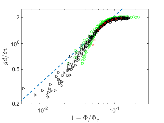


We notice that when the packing fraction is less than 0.57, the data points lay on a single curve, however, as the packing fraction increases, different cases have different curves. Interestingly, the normalized fluidity proposed in the main text and shown in FIG. 5(c) collapses the same data more strongly, which suggests the kinetic pressure formula used in the former test may be less reliable in dense, non-uniform flow fields. This point is discussed in more depth next.
Possible simplifications of
An equation of state relating the pressure, volume and temperature (PVT relationship) is a common assumption in fluids. In the hypothesized formula for , corresponds to “V” and corresponds to “T”. In the following, we discuss possible relations between , and to see if one of the independent variables in the hypothesis can be replaced with , thereby reducing the number of physical kinematic variables introduced to one. Alternatively, it is also natural to ask if one of the independent variables tends to be ‘relatively constant’ compared to the other, such that the profile of can be discerned largely from either or . We consider these possibilities next.
- 1.
Is it possible or ?
If we are only allowed to use and as the independent variables, then there are two dimensionless numbers: and , where is the solid density of the grains. FIG. 6(a) shows that fluidity is not generally well described solely by and .
Considering and as the independent variables, we can get two dimensionless numbers: and . FIG. 6(b) shows that fluidity is not generally well described solely by and .
These suggest a non-unique relationship between , and in dense inhomogeneous flows. In the absence of any dimensional constant, using , and , we can get two dimensionless numbers: and . Existence of a PVT equation of state would thus imply a one-to-one relation between and . As plotted in FIG. 6(c) such an equation of state does not collapse out of the data from our many tests in inhomogeneous flows. In particular, the spread is most evident for high packing fractions where a larger role for cooperativity exists, conceivably influencing the interrelationship between these variables. It is certainly the case that for static, dense packings, the density and pressure need not related uniquely for hard particles.
- 2.
Is typically sensitive both to and to , or is one variable dominant?
As shown in the main text, the collapse of onto spans an order of magnitude. Hence, at hypothetically fixed velocity fluctuations, the fluidity would still be nontrivially influenced by in typical flows. The fluidity is proportional to at fixed , so nontrivial variations in would cause nontrivial variations in . Unlike equilibrium materials where internal temperature rapidly equilibrates with an external bath, all fluctuations in granular flow are generated from plastic flow itself, absent wall vibrations. This can produce largely inhomogeneous spatial fields for , varying one or more orders of magnitude in typical flows [5, 7]. Hence, cannot be treated as a relatively constant field for the purposes of computing granular fluidity in an arbitrary flow.
As a direct example, the depth profiles of velocity in inclined plane flow geometries having the same inclination angle but different heights of the granular layers differ from each other [4], whereas the packing fraction and profiles are quite homogeneous and almost at the same value through all cases. Because , the observed variations in strain-rate imply is not adequate on its own to describe the granular fluidity in inclined flows. The inclined flow cases show that the effect of is not negligible and is generally not able to be simplified further.


References
- [1] B. Andreotti, Y. Forterre, and O. Pouliquen, Granular media: between fluid and solid (Cambridge University Press, 2013).
- [2] F. da Cruz, S. Emam, M. Prochnow, J.-N. Roux, and F. Chevoir, Physical Review E 72, 021309 (2005).
- [3] P. Jop, Y. Forterre, and O. Pouliquen, Journal of Fluid Mechanics 541, 167 (2005).
- [4] L. E. Silbert, J. W. Landry, and G. S. Grest, Physics of Fluids (1994-present) 15, 1 (2003).
- [5] G. MiDi, The European Physical Journal E 14, 341 (2004).
- [6] F. Da Cruz, F. Chevoir, D. Bonn, and P. Coussot, Physical Review E 66, 051305 (2002).
- [7] G. Koval, J.-N. Roux, A. Corfdir, and F. Chevoir, Physical Review E 79, 021306 (2009).
- [8] K. Reddy, Y. Forterre, and O. Pouliquen, Physical Review Letters 106, 108301 (2011).
- [9] K. Nichol, A. Zanin, R. Bastien, E. Wandersman, and M. van Hecke, Phys. Rev. Lett. 104, 078302 (2010).
- [10] F. Radjai and S. Roux, Physical Review Letters 89, 064302 (2002).
- [11] O. Pouliquen, Physical review letters 93, 248001 (2004).
- [12] G. Lois, A. Lemaitre, and J. Carlson, EPL (Europhysics Letters) 76, 318 (2006).
- [13] L. Staron, Physical Review E 77, 051304 (2008).
- [14] L. Staron, P.-Y. Lagrée, C. Josserand, and D. Lhuillier, Physics of Fluids (1994-present) 22, 113303 (2010).
- [15] M. Bouzid, M. Trulsson, P. Claudin, E. Clément, and B. Andreotti, Physical review letters 111, 238301 (2013).
- [16] K. Kamrin and G. Koval, Physical Review Letters 108, 178301 (2012).
- [17] D. L. Henann and K. Kamrin, Proceedings of the National Academy of Sciences 110, 6730 (2013).
- [18] K. Kamrin and G. Koval, Computational Particle Mechanics 1, 169 (2014).
- [19] D. L. Henann and K. Kamrin, International Journal of Plasticity 60, 145 (2014a).
- [20] D. L. Henann and K. Kamrin, Physical review letters 113, 178001 (2014b).
- [21] K. Kamrin and D. L. Henann, Soft matter 11, 179 (2015).
- [22] This the full form of the granular fluidity relation; an approximation for steady-state solutions only is also commonly used [16, 17].
- [23] M. Bouzid, A. Izzet, M. Trulsson, E. Clément, P. Claudin, and B. Andreotti, The European Physical Journal E 38, 1 (2015).
- [24] L. Bocquet, W. Losert, D. Schalk, T. Lubensky, and J. Gollub, Physical review E 65, 011307 (2001).
- [25] Y. Forterre and O. Pouliquen, Physical Review Letters 86, 5886 (2001).
- [26] B. Utter and R. Behringer, Physical review letters 100, 208302 (2008).
- [27] R. Artoni and P. Richard, Physical review letters 115, 158001 (2015a).
- [28] S. Plimpton, Journal of computational physics 117, 1 (1995).
- [29] See Supplemental Material for more details of the averaging methodology, verifications of the averaging method, detailed comparisons with kinetic theory, and further discussion on whether can be reduced.
- [30] The value of is irrelevant here, as we study only steady-state.
- [31] C. Lun, S. Savage, D. Jeffrey, and N. Chepurniy, Journal of fluid mechanics 140, 223 (1984).
- [32] J. T. Jenkins and D. Berzi, Granular Matter 12, 151 (2010).
- [33] W. Losert, L. Bocquet, T. Lubensky, and J. P. Gollub, Physical review letters 85, 1428 (2000).
- [34] H. Eyring, The Journal of chemical physics 4, 283 (1936).
- [35] F. Spaepen, Acta metallurgica 25, 407 (1977).
- [36] O. Pouliquen and Y. Forterre, Philosophical Transactions of the Royal Society of London A: Mathematical, Physical and Engineering Sciences 367, 5091 (2009).
- [37] F. Radjai, S. Roux, and J. J. Moreau, Chaos: An Interdisciplinary Journal of Nonlinear Science 9, 544 (1999).
- [38] D. M. Mueth, H. M. Jaeger, and S. R. Nagel, Physical Review E 57, 3164 (1998).
- [39] T. S. Majmudar and R. P. Behringer, Nature 435, 1079 (2005).
- [40] K. Kamrin and E. Bouchbinder, Journal of the Mechanics and Physics of Solids 73, 269 (2014).
- [41] M. H. Cohen and D. Turnbull, The Journal of Chemical Physics 31, 1164 (1959).
- [42] L. Bocquet, A. Colin, and A. Ajdari, Physical review letters 103, 036001 (2009).
- [43] P. Jop, V. Mansard, P. Chaudhuri, L. Bocquet, and A. Colin, Physical Review Letters 108, 148301 (2012).
- [44] R. Artoni and P. Richard, Physical Review E 91, 032202 (2015b).
- [45] P. Haff, Journal of Fluid Mechanics 134, 401 (1983).