Tracking Switched Dynamic Network Topologies
from Information Cascades†
Abstract
Contagions such as the spread of popular news stories, or infectious diseases, propagate in cascades over dynamic networks with unobservable topologies. However, “social signals” such as product purchase time, or blog entry timestamps are measurable, and implicitly depend on the underlying topology, making it possible to track it over time. Interestingly, network topologies often “jump” between discrete states that may account for sudden changes in the observed signals. The present paper advocates a switched dynamic structural equation model to capture the topology-dependent cascade evolution, as well as the discrete states driving the underlying topologies. Conditions under which the proposed switched model is identifiable are established. Leveraging the edge sparsity inherent to social networks, a recursive -norm regularized least-squares estimator is put forth to jointly track the states and network topologies. An efficient first-order proximal-gradient algorithm is developed to solve the resulting optimization problem. Numerical experiments on both synthetic data and real cascades measured over the span of one year are conducted, and test results corroborate the efficacy of the advocated approach.
Index Terms:
Social networks, structural equation model, network cascade, topology inference, switched linear systems.I Introduction
Information often spreads in cascades by following implicit links between nodes in real-world networks whose topologies may be unknown. For example the spread of viral news among blogs, or Internet memes over microblogging tools like Twitter, are facilitated by the inherent connectivity of the world-wide web. A celebrity may post an interesting tweet, which is then read and retweeted by her followers. An information cascade may then emerge if the followers of her followers share the tweet, and so on. The dynamics of propagation of such information over implicit networks are remarkably similar to those that govern the rapid spread of infectious diseases, leading to the so-termed contagions [21, 7, 1]. Similar cascading processes have also been observed in the context of adoption of emerging fashion trends within distinct age groups, the successive firing of thousands of neurons in the brain in response to stimuli, and plummeting stock prices in global financial markets in response to a natural disaster.
Cascades are generally observed by simply recording the time when a specific website first mentioned a cascading news item, or when an infected person first showed symptoms of a disease. On the other hand, the underlying network topologies may be unknown and dynamic, with the link structure varying over time. Unveiling such dynamic network topologies is crucial for several reasons. Viral web advertising can be more effective if a small set of influential early adopters are identified through the link structure, while knowledge of the structure of hidden needle-sharing networks among communities of injecting drug users can aid formulation of policies for curbing contagious diseases. Other examples include assessment of the reliability of heavily interconnected systems like power grids, or risk exposure among investment banks in a highly inter-dependent global economy. In general, knowledge of topologies that facilitate diffusion of network processes leads to useful insights about the behavior of complex systems.
Network contagions arise due to causal interactions between nodes e.g., blogs, or disease-susceptible individuals. Structural equation models (SEMs) effectively capture such causal relationships, that are seldom revealed by symmetric correlations; see e.g., [10, 18]. Widely applied in psychometrics [15], and sociometrics [8], SEMs have also been adopted for gene network inference [5, 12], and brain connectivity studies [13]. Recently, dynamic SEMs have been advocated for tracking slowly-varying sparse social network topologies from cascade data [1].
Network topologies may sometimes “jump” between a finite number of discrete states, as manifested by sudden changes in cascade behavior. For example, an e-mail network may switch topologies from predominantly work-based connections during the week, to friend-based connections over the weekend. Connection dynamics between bloggers may switch suddenly at the peak of sports events (e.g., “Superbowl”), or presidential elections. In such settings, contemporary approaches assuming that network dynamics arise as a result of slow topology variations may yield unpredictable results. The present paper capitalizes on this prior knowledge, and puts forth a novel switched dynamic SEM to account for propagation of information cascades in such scenarios. The novel approach builds upon the dynamic SEM advocated in [1], where it is tacitly assumed that node infection times depend on both the switching topologies and exogenous influences e.g., external information sources, or prior predisposition to certain cascades.
The present paper draws connections to identification of hybrid systems, whose behavior is driven by interaction between continuous and discrete dynamics; see e.g., [16] and references therein. Switched linear models have emerged as a useful framework to capture piecewise linear input-output relations in control systems [2, 22, 23]. The merits of these well-grounded approaches are broadened here to temporal network inference from state-driven cascade dynamics. Although the evolution of the unknown network state sequence may be controlled by structured hidden dynamics (e.g., hidden Markov models), this work advocates a more general framework in which such prior knowledge is not assumed.
Network inference from temporal traces of infection events has recently emerged as an active research area. A number of approaches put forth probabilistic models for information diffusion, and leverage maximum likelihood estimation (MLE) to infer both static and dynamic edge weights as pairwise transmission weights between nodes [20, 19, 14]. Sparse SEMs are leveraged to capture exogenous inputs in inference of dynamic social networks in [1], and static causal links in gene regulatory networks [5]. Network Granger causality with group sparsity is advocated for inference of causal networks with inherent grouping structure in [3], while causal influences are inferred by modeling historical network events as multidimensional Hawkes processes in [25].
Within the context of prior works on dynamic network inference, the contributions of the present paper are three-fold. First, a novel switched dynamic SEM that captures sudden topology changes within a finite state-space is put forth (Section II). Second, identifiability results for the proposed switched model are established under reasonable assumptions, building upon prior results for static causal networks in [4] (Section III). Finally, an efficient sparsity-promoting proximal-gradient (PG) algorithm is developed (Sections IV and V) to jointly track the evolving state sequence, and the unknown network topologies. Numerical tests on both synthetic and real cascades in Section VI corroborate the efficacy of the novel approach. Interestingly, experiments on real-world web cascade data exemplify that media influence is dominated by major news outlets (e.g., cnn.com and bbc.com), as well as well-known web-based news aggregators (e.g., news.yahoo.com and news.google.com).

Notation. Bold uppercase (lowercase) letters will denote matrices (column vectors), while operators , , and will stand for matrix transposition, maximum eigenvalue, and diagonal matrix, respectively. The identity matrix will be represented by , while will denote the matrix of all zeros, and their dimensions will be clear in context. Finally, the and Frobenius norms will be denoted by , and , respectively.
II Model and Problem Statement
Consider a dynamic network with nodes observed over time intervals , captured by a graph whose topology may arbitrarily switch between discrete states. Suppose the network topology during interval is described by an unknown, weighted adjacency matrix , with . Entry of (henceforth denoted by ) is nonzero only if a directed edge connects nodes and (pointing from to ) during interval . In general , i.e., matrix is generally non-symmetric, which is suitable to model directed networks. The model tacitly assumes that the network topology remains fixed during any given time interval , but can change across time intervals.
Suppose contagions propagating over the network are observed, and the time of first infection per node by contagion is denoted by . In online media, can be obtained by recording the timestamp when blog first mentioned news item . If a node remains uninfected during , is set to an arbitrarily large number. Assume that the susceptibility of node to external (non-topological) infection by contagion is known and time invariant. In the web context, can be set to the search engine rank of website with respect to (w.r.t.) keywords associated with .

The infection time of node during interval is modeled according to the following switched dynamic structural equation model (SEM)
| (1) |
where captures the state-dependent level of influence of external sources, and accounts for measurement errors and unmodeled dynamics. It follows from (1) that if , then is affected by the values of (see Figure 2). With diagonal , collecting observations for the entire network and all contagions yields the dynamic matrix SEM
| (2) |
where , , and are all matrices. A single network topology is adopted for all contagions, which is suitable e.g., when information cascades are formed around a common meme or trending (news) topic over the Internet. Matrix has an all-zero diagonal to ensure that the underlying network is free of self loops, i.e., .
Problem statement. Given the sequence and adhering to (2), the goal is to identify the unknown state matrices , and the switching sequence .
III Model Identifiability
This section explores the conditions under which one can uniquely recover the unknown state matrices . First, (2) can be written as
| (3) |
where the binary indicator variable if , otherwise . Note that (3) is generally underdetermined when is unknown, and it may not be possible to uniquely identify . Even in the worst-case scenario where , complete identification of all states is impossible if there exists and () such that . In order to establish model identifiability, it will be assumed that the following hold:
as1. The dynamic SEM in (2) is noise-free (); that is,
| (4) |
as2. All cascades are generated by some pair , where , and is known. This is a realizability assumption, which guarantees the existence of a submodel responsible for the observed cascades.
as3. No two states can be active during a given time interval, i.e., implies that .
Under (as1)-(as3), the following proposition holds.
Proposition 1: Suppose data matrices and adhere to (4) with , , and . If and has full row rank, then and are uniquely expressible in terms of and as , and .
If denotes the activation probability of state , with , and (as1)-(as3) hold, then can be uniquely identified with probability one as .
Proposition III establishes a two-step identifiability result for the dynamic SEM model in (4). First, it establishes that if the exogenous data matrix is sufficiently rich (i.e., has full row rank), then the per-interval network topology captured by can be uniquely identified per . Second, if the state activation probabilities are all strictly positive, then the switching network topologies will all be recovered as . In fact, if cascade data are acquired in an infinitely streaming fashion (), then one is guaranteed to uniquely recover all states.
Proof of Proposition III: Equation (4) can be written as , which implies that . With and both having full row rank (recall that ), it follows that has full row rank, and is invertible. Consequently, the linear system of equations is solved by .
On the other hand, note that admits the solution
| (5) |
which is unique since is full row rank. Since and is a diagonal matrix, the diagonal entries of coincide with those of ; hence, , which leads to
| (6) |
upon substitution of (5). Furthermore, note that , and thus
| (7) |
which concludes the first part of the proof.
Since and , the results from the unique solutions (6) and (7) coincide with a specific pair in the set per . Intuitively, complete recovery of all state matrices is tantamount to identification of unique pairs as more data are sequentially acquired. In order to guarantee identifiability of all states in the long run, it suffices to prove that the probability of activation of any state at least once tends to as . Since are Bernoulli random variables with per , the number of times that state is activated over time intervals follows a binomial distribution. Letting denote the total number of activations of state over , then
| (8) | |||||
Since only if , it follows that all states can be uniquely identified with probability as when , which completes the second part of the proof.
III-A Topology tracking by clustering when
In general, even when is full row rank, in order to compensate for measurement errors and unmodeled dynamics. Under noisy conditions, it will turn out that can be interpreted as cluster centroids (cf. (3)), and one can leverage traditional clustering approaches (e.g., k-means), coupled with the closed-form solutions in (6) and (7) to identify the unknown state matrices. Indeed, with , and , it follows readily that
| (9) |
where , and .
Clearly, in (9) can be viewed as cluster centers, and as unknown binary cluster-assignment variables. Consequently, the sequence can be directly computed per via (6) and (7), where denotes the number of training samples. Identification of and can then be accomplished by batch clustering into clusters. The subsequent operational phase () then boils down to computing , followed by finding the centroid to which it is closest in Euclidean distance, that is
| (10) |
and if , otherwise . Algorithm 1 summarizes this cluster-based state identification scheme, with a clustering phase () and an operational phase (). The sub-procedure calls an off-the-shelf clustering algorithm with the training set and the number of clusters as inputs.
Remark 1
Algorithm 1 identifies the unknown state-dependent matrices by resorting to “hard clustering,” which entails deterministic assignment of to one of the centroids. In principle, the algorithm can be readily modified to adopt “soft clustering” approaches, with probabilistic assignments to the cluster centroids.
IV Exploiting edge sparsity
The fundamental premise established by Proposition III is that are uniquely identifiable provided is sufficiently rich. However, requiring that has full row rank is a restrictive condition, tantamount to requiring that at least as many cascades are observed as the number of nodes (). This is especially prohibitive in large-scale networks such as the world-wide web, with billions of nodes. It is therefore of interest to measure as few cascades as possible while ensuring that are uniquely recovered. To this end, one is motivated to leverage prior knowledge about the unknowns in order to markedly reduce the amount of data required to guarantee model identifiability. For example, each node in the network is connected only to a small number of nodes out of the possible connections. As a result, most practical networks exhibit edge sparsity, a property that can be exploited to ensure that the rank condition on can be relaxed, as shown in the sequel. In addition to (as1)-(as3), consider the following.
as4. Each row of matrix has at most nonzero entries; i.e., .
as5. The nonzero entries of for all are drawn from a continuous distribution.
as6. The Kruskal rank of satisifies , where is defined as the maximum number such that any combination of columns of constitute a full column rank submatrix.
Proposition 2: Suppose data matrices and adhere to (4) with , , and . If (as1)-(as6) hold, and , then can be uniquely identified with probability one as .
The proof of Proposition IV is rather involved, and is deferred to Appendix A. Unlike the matrix rank which only requires existence of a subset of linearly independent columns, the Kruskal rank requires that every possible combination of a given number of columns be linearly independent. Moreover, computing is markedly more challenging, as it entails a combinatorial search over the rows of . Admittedly, requiring is more restrictive than . Nevertheless, in settings where , (as6) may be satisfied even if . In such cases, Proposition IV asserts that one can uniquely identify even when .
IV-A Sparsity-promoting estimator
The remainder of the present paper leverages inherent edge sparsity to develop an efficient algorithm to track switching network topologies from noisy cascade traces. Assuming is known a priori, one is motivated to solve the following regularized LS batch estimator
| s. to | (11) | ||||
where the constraint enforces a realizability condition, ensuring that only one state can account for the system behavior at any time. With , the regularization term promotes edge sparsity that is inherent to most real networks. The sparsity level of is controlled by . Absence of a self-loop at node is enforced by the constraint , while having , ensures that is diagonal as in (2).
Note that (P0) is an NP-hard mixed integer program that is unsuitable for large-scale and potentially real-time operation. Moreover, entries of per-state matrices may evolve slowly over reasonably long observation periods, motivating algorithms that not only track the switching sequence, but also the slow drifts occurring in per-state network topologies.
Suppose data are sequentially acquired, rendering batch estimators impractical. If it is assumed that instantaneous and past estimates of are known during interval , (P0) decouples over , and is tantamount to solving the following subproblem per and
| s. to | (12) |
Note that the LS term in the penalized cost only aggregates residuals when . In principle, during interval , (P1) updates the estimates of and only if has been generated by submodel . Critical to efficiently tracking the hidden network topologies is the need for a reliable approach to estimate . Before developing an efficient tracking algorithm that will be suitable to solve (P1), the rest of this section puts forth criteria for estimating .
Estimation of . Given the most recent estimates prior to acquisition of , one can estimate by minimizing the a priori error over i.e.,
| (13) |
followed by solving (P1) with . If network dynamics arise from switching between static or slowly-varying per-state topologies, (13) yields a reliable estimate of the most likely state sequence over time.
Alternatively, one may resort to a criterion that depends on minimizing the a posteriori error. This entails first solving (P1) for all states upon acquisition of , and then selecting so that
| (14) |
where (resp. ) denotes the estimate of (resp. ) given that . In the context of big data and online streaming, (14) is prohibitive, and (13) is more desirable for its markedly lower computational overhead. The tracking algorithm developed next adopts (13) for state sequence estimation.
V Topology Tracking Algorithm
In order to solve (P1), this section resorts to proximal gradient (PG) approaches, which have been popularized for -norm regularized problems, through the class of iterative shrinkage-thresholding algorithms (ISTA); see e.g., [6] and [17]. Unlike off-the-shelf interior point methods, ISTA is computationally simple, with iterations entailing matrix-vector multiplications, followed by a soft-thresholding operation [9, p. 93]. Motivated by its well-documented merits, an ISTA algorithm is developed in the sequel for recursively solving (P1) per . Memory storage and computational costs incurred by the algorithm per acquired sample do not grow with .
Solving (P1) for a single time interval . Introducing the optimization variable , it follows that the gradient of is Lipschitz continuous, meaning there exists a constant so that , in the domain of . Instead of directly optimizing the cost in (P1), PG algorithms minimize a sequence of overestimators evaluated at the current iterate, or a linear combination of the two previous iterates.
Letting denote the iteration index, and , PG algorithms iterate
| (15) |
where corresponds to a gradient-descent step taken from , with step-size equal to . The optimization problem (15) is denoted by , and is known as the proximal operator of the function evaluated at . With for convenience, the PG iterations can be compactly rewritten as .
The success of PG algorithms hinges upon efficient evaluation of the proximal operator (cf. (15)). Focusing on (P1), note that (15) decomposes into
| (16) | ||||
| (17) |
subject to the constraints in (P1) which so far have been left implicit, and . Letting with -th entry given by denote the soft-thresholding operator, it follows that , see e.g., [6, 9]. Since there is no regularization on , (17) boils-down to a simple gradient-descent step.
Specification of and only requires expressions for the gradient of with respect to and . Note that by incorporating the constraints and , one can express as
| (18) |
where and denote the -th row of and , respectively; while denotes the vector obtained by removing entry from the -th row of , and likewise is the matrix obtained by removing row from . It is apparent from (18) that is separable across the trimmed row vectors , and the diagonal entries , . The sought gradients are
| (19) | ||||
| (20) |
where denotes the -th row of , , and . Similarly, and is obtained by removing the -th row and -th column from . From (16)-(17) and (19)-(20), the parallel ISTA iterations
| (21) | ||||
| (22) | ||||
| (23) | ||||
| (24) |
are provably convergent to the globally optimal solution of (P1), as per general convergence results for PG methods [6, 17].
Note that iterations (23)-(24) incur a low computational overhead, involving at most matrix-vector multiplication complexity for the gradient evaluations. A final step entails zero-padding the updated by setting
| (25) |
The desired SEM parameter estimates are subsequently obtained as and , for large enough so that convergence has been attained.
Solving (P1) over the entire time horizon. Tracking the switching sequence and the state parameters entails sequentially alternating between two operations per datum arrival. First, is estimated (via solving (13) or (14)), and the corresponding values are accordingly obtained. The iteration steps (21)-(24) are then run until convergence is attained. Note that these iterations only depend on past data through recursively updated moving averages, that is,
| (26) |
Similar recursive expressions can be readily derived for , and . The complexity in evaluating the Gram matrix dominates the per-iteration computational cost of the algorithm. The recursive updates in (26) are conducted only for a single state per interval , with the remainder set to . Similarly, iterations (21)-(24) are run only for , while are not updated during interval . Furthermore, the need to recompute per can be circumvented by selecting an appropriate step-size for (23)-(24) by line search [17].
Algorithm 2 summarizes the developed state-dependent topology tracking scheme. Numerical tests indicate that inner ISTA iterations suffice to track the evolving topology remarkably well.
V-A Initialization of Algorithm 2
In order to run Algorithm 2, one needs initial state estimates . If is known to have full row rank, Algorithm 1 can be used to initialize the state matrices as the cluster centroids. However, this is quite restrictive, and a more general initialization scheme can be obtained with less stringent restrictions on . For example, the following regularized LS estimator with
| (27) |
yields estimates per for a designated initialization interval (). The initializations are then obtained as the cluster centroids of . Note that (27) decouples across nodes, and amounts to solving
| (28) |
for . Indeed, (28) admits the following per-variable closed-form solutions
| (29) |
and
| (30) |
for . Starting with an initial value for , one can compute (29) and (30) in an alternating fashion by fixing one variable and updating the other, until convergence is attained.
V-B Tracking slowly-changing state matrices
It has tacitly been assumed that state matrices are static, and that temporal dynamics only arise from the switching sequence . Nevertheless, entries of each of the state matrices may drift slowly over time, motivating algorithms that down-weigh the influence of past data. To this end, (P1) can be modified as follows
| s. to | (31) |
where is a forgetting factor that exponentially down-weighs past data whenever . In order to solve (P2), Algorithm 2 can be readily modified in a reasonably straight-forward manner, and details are omitted here for brevity.
VI Numerical Tests
VI-A Synthetic Data
Data generation. To assess the performance of the developed algorithms, the first set of experiments were conducted on synthetic cascade data. Four Kronecker graphs were generated from the following seed matrices [11]
The resulting graph adjacency matrices , each encoding a network of nodes, were obtained by repeated Kronecker products for . Each diagonal entry of was set to zero, while the number of cascades was set to , and time intervals to . Furthermore, was constructed with entries sampled from a uniform distribution as . Similarly, the diagonal matrices were constructed by sampling entries from a uniform distribution as . Synthetic cascade data were then generated as , with sampled uniformly at random from per , and , for . Figure 3 (a) depicts the ground-truth adjacency matrices used to generate the synthetic cascade data.
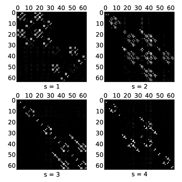
Experimental results. First, Algorithm 1 was run with , and k-means as the clustering algorithm of choice. Figure 3 (b) depicts heatmaps of the resulting adjacency matrices obtained as cluster centroids. Note that Algorithm 1 is devoid of a data-driven thresholding scheme, hence most entries in the recovered adjacency matrix are nonzero. Nevertheless, visual inspection of the heatmaps reveals that larger entries generally correspond to non-zero edge weights as shown in Figure 3 (a). Since the synthetic cascade data are noisy, it is not surprising that Algorithm 1 exhibits suboptimal topology identification. In fact as demonstrated next, Algorithm 2 is markedly superior to Algorithm 1 with respect to coping with noise, as well as shrinking non-edge entries of to zero.
Using the initial cascade samples , per-interval state-agnostic batch estimates were obtained by solving (27) with . The estimates were then clustered via the k-means algorithm, with clusters, and the corresponding cluster centers were used as the initial values . Algorithm 2 was then run for , with , and . Figure 3 (c) depicts heatmaps of the recovered state-dependent adjacency matrices at . Thanks to sparsity regularization, Algorithm 2 unveils the non-zero support structures of the state matrices with remarkable success. Figure 4 plots the actual and estimated switching sequences from to , clearly demonstrating the remarkable success in tracking the underlying states.
Next, the advocated approach was compared with earlier work which models temporal information cascades using dynamic SEMs, with slow topology variations [1]. A stochastic gradient descent (SGD) algorithm developed in [1] was run with batch initialization on the time-series of cascade data. Per interval , the resulting relative estimation error, , was evaluated for both Algorithm 2 and the SGD tracker from [1]. Note that in computing the estimation error for Algorithm 2, (similarly for and ). Figure 5 (a) compares the per-interval relative errors of the two approaches. It is clear from the plot that exploiting the prior knowledge that network dynamics arise due to random switching between states yields remarkably superior error performance than the alternative. In fact, the final adjacency matrix does not correspond to a specific state, but is rather an average of the underlying state matrices. However, this is not surprising since the framework advocated in [1] exploits slow topology variations, and it is not expected to outperform algorithms developed in the present paper, when topologies potentially jump suddenly between discrete states.
To this end, a new slowly-varying state sequence was used to control the evolving network topologies, and a new time series of synthetic cascades was generated. Specifically, the following scheme was used to generate a piecewise-constant sequence :
while the ground-truth matrices and remained unchanged. Figure 5 (a) compares per-interval relative errors resulting from running Algorithm 2, and the SGD algorithm developed in [1]. In this case, there are fewer sudden transitions between network states. Nevertheless, leveraging the prior information about the state-based network evolution is beneficial as shown by the plot. Indeed, modeling cascade propagation by the proposed switched dynamic SEM framework leads to better error performance than adopting a state-incognizant approach that exploits the underlying slow variations.

(a)

(b)
(c)


(a)

(b)
VI-B Real Cascade Data
Dataset description. This section presents results of experimental tests conducted on real cascades observed on the web between March and February . Blog posts and news articles for memes (popular textual phrases) appearing within on approximately million websites were monitored during the observation period. The time when a given website first mentioned a story related to a specific set of memes was recorded, and the data were availed to the public from [InfoPath]. Cascade infection times were recorded as Unix timestamps in hours (i.e., the number of hours since midnight on January , ). Several trending news topics during this period were identified, and cascade data for the top websites that mentioned memes associated with them were retained. From this dataset, cascades related to broad news topics were extracted for the present paper’s experiments. Table I lists the names of these topics, with a correspondingly brief description.
| Broad news topic | Brief description | |
|---|---|---|
| 1 | Fukushima | Nuclear accident at Japan’s Fukushima nuclear power plant in March 2011 |
| 2 | Kate Middleton | English royal whose wedding took place in April 2011 |
| 3 | Kim Jong-un | Leader of North Korea who rose to prominence upon the death of his father in December 2011 |
| 4 | Osama bin Laden | Infamous terrorist leader who was killed in May 2011 |
| 5 | Amy Winehouse | Famous English singer who died of drug overdose in July 2011 |
| 6 | Rupert Murdoch | Businessman whose media company was involved in a phone hacking scandal revealed in May 2011 |
| 7 | Steve Jobs | Technology entrepreneur whose death in October 2011 was followed by many news headlines |
| 8 | Arab spring | Wide-spread politically-charged protests among several Arab nations starting in December 2010 |
| 9 | Strauss Kahn | International Monetary Fund (IMF) director who resigned in May 2011 due to sex assault allegations |
| 10 | Reid Hoffman | Founder of LinkedIn whose stock started trading in May 2011 |
For each broad topic in Table I, many news stories appeared on blogs and mainstream news websites over the observation period. Each story was assigned a list of tuples in the form (website id, timestamp) capturing the time when it was first mentioned on a particular website. For the present paper, a popular news story was characterized as a meme if it propagated to at least websites, due to repeated mentions. Based on this definition, all news stories that did not qualify as memes were discarded, and a total of cascades constituting the selected memes, and their infection times were retained. Due to this thresholding, the total number of of websites reduced to . The observation period was split into time intervals , each corresponding to approximately days. Letting denote the Unix infection time of node by cascade , datum was computed as follows:
| (32) |
only if , otherwise is set to a very large value, namely , as a surrogate for infinity.
Entries of capture prior knowledge about the susceptibility of each node to each contagion. For instance, the entry could denote the online search rank of website for a search keyword associated with contagion . In the absence of such website ranking information, the present paper resorted to an alternative approach involving assignment of susceptibilities from the entire corpus of the cascade data. First, five broad categories of memes were identified as politics, entertainment, sports, business, and technology, and indexed by . Each group of news topics was manually labeled using these five prescribed categories. Next, for each website , was computed as follows
for all categories. Entry was then set to if cascade belonged to category .
Experimental results. Since is unknown for the real dataset, the first part of this experimental test entailed approximating its value from the data. Setting , the initialization scheme in (27) was run in batch mode over intervals. The resulting estimates of were then clustered using -means, with . For each , the total intra-cluster distance was evaluated upon convergence as
| (33) |
on a logarithmic scale, with the estimates , and defined earlier. Figure 7 plots for , depicting a substantial decrease from to . Subsequent values of do not markedly reduce . From this plot, was selected as the underlying number of network states.
Next, Algorithm 2 was run with the pre-processed cascade data as inputs. Note that Algorithm 2 requires the sparsity-promoting regularization parameters as inputs. In this experiment, a uniform value was adopted for all states, i.e., . In the absence of ground-truth state topologies, selection of is rather challenging, and it remains an open question for future work. Nevertheless, a heuristic approach inspired by typical properties of real-world large-scale networks was adopted for the present paper. Over the last years, several studies in network science have unveiled remarkable universal properties that seem to underlie most real networks. For example, networks generally exhibit the so-termed “small-world” property, and their degree distributions often follow power laws [24].
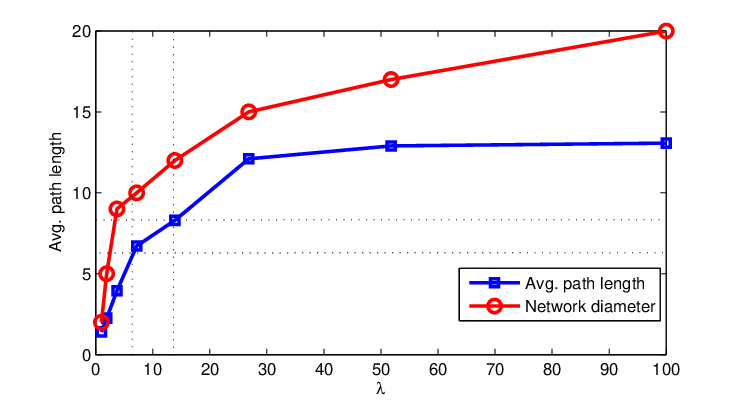
Acknowledging these as universal laws inherent to most networks, it is possible to constrain the search space of the most likely network topologies uncovered by Algorithm 2. In this experiment, was selected in such a way that the average shortest path length between any pair of nodes is , which is consistent with the “small-world” phenomenon. With , the goal was to select so that the resulting average shortest path length was within the interval . For each , Algorithm 2 was run and the average shortest path lengths were computed per network state, and then averaged over all states. Figure 8 plots the average path length as is varied between and . The plot also depicts the corresponding average network diameters, which can also be used as a validation metric. It turns out that setting for led to an average shortest path length of approximately , which is indicative of an underlying “small-world” property. Table II summarizes the per-state average clustering coefficient, network diameter, average number of neighbors, and the average shortest path length when .

(a)

(b)

(c)


| Network state | 1 | 2 | 3 |
|---|---|---|---|
| Average clustering coefficient | |||
| Network diameter | |||
| Average number of neighbors | |||
| Average shortest path length |
Figure 6 depicts visualizations of the state-dependent network topologies inferred from the cascade data using Algorithm 2. Each drawing is annotated with the top websites when ranked in order of decreasing out-degree. It is interesting to note that this list is dominated by websites corresponding to the most influential news outlets in the English-speaking world e.g., nytimes.com, cnn.com, bbc.co.uk, and theguardian.com. Furthermore, it turns out that popular news aggregators, such as news.yahoo.com and news.google.com, are competitive with traditional media powerhouses in terms of influencing the propagation of news over the web. Although this analysis only considers English-based websites, these experimental results on real-world cascades are strongly corroborated by prior expectations about the most influential enablers of information propagation over the world-wide web. Finally, Figure 9 depicts the switching sequence for the network topologies over the entire observation period. It turns out that evolution of the network topology adheres to piecewise constant state variations.
VII Conclusion
A switched dynamic SEM was proposed for tracking the evolution of dynamic networks from information cascades when topologies arbitrarily switch between discrete states. It was shown that presence of exogenous influences is critical to guarantee model identifiability, and one can even identify the underlying network topologies with fewer cascade measurements by leveraging edge sparsity. Recognizing that identification of the unknown network states and the switching sequence is computationally challenging, the present paper assumed that the number of states are known a priori, and advocated an exponentially-weighted LS estimator capitalizing on edge sparsity. A recursive two-step topology tracking algorithm leveraging advances in proximal gradient optimization was developed. Per interval, the first step estimates the active state by minimizing the a priori prediction error, while the second step recursively updates only the matrices corresponding to the estimated state.
Experiments on synthetically-generated cascades demonstrated the effectiveness of the advocated approach in jointly tracking the switching sequence, while identifying the state-dependent network topologies. Numerical tests were also conducted on real cascades of popular news over the web, collected over one year. The goal was to identify the underlying topological structure of causal influences between news websites and blogs. Interestingly, websites exhibiting the highest influence (as measured by the out-degree) turned out to be recognizable news outlets and popular news aggregators. Future directions include investigation of more efficient approaches for tracking the switching sequence, identification of the number of states, and selection of sparsity-promoting parameters, especially when ground-truth network topologies are unknown.
Appendix A Proof of Proposition IV
In order to construct the proof for Proposition IV, it is necessary to state and prove Lemmas A and A.
Lemma 1: Under (as5), matrix is invertible with probability one.
Proof: Note that is a polynomial whose variables are the nonzero entries of . Consequently, for some constants , the probability that is not invertible can be equivalently written as
| (34) |
Since is drawn from a continuous distribution (as5), it follows that , implying that .
Lemma 2: Under (as4)-(as6), assuming , implies that
with probability one.
Proof: Defining , note that . Let denote a submatrix of , formed by selecting an arbitrary subset of columns indexed by the set whose cardinality is . Given that , there exists a set of rows of indexed by with cardinality , such that the resulting square submatrix has full rank.
Since from Lemma A, we have that is invertible, it holds that , or , where . Collecting the columns and rows of indexed by and into , it follows that , where collects rows of indexed by , and collects columns of indexed by . Equivalently, one can write , where only the corresponding columns of and rows of are retained.
By Cramer’s rule for matrix inversion, entry of can be written as , where denotes a polynomial function of degree at most , with nonzero entries of as variables. Furthermore, the entries of are linear combinations of entries of , while the determinant of is a polynomial of degree , with its entries as variables. As a result, one can write the determinant of as
| (35) |
where is a polynomial of degree at most with nonzero entries of as variables, and is formed by the composition of the polynomials and linear combinations of entries of .
It can be shown that is not identically zero as follows. Since implies that , then , because is full rank by construction. Consequently, depends on nonzero entries of , which are drawn from a continuous distribution. Similar to the argument made in the proof of Lemma A, the probability that is zero. Since has full rank, then with probability one.
Proposition 2: Suppose data matrices and adhere to (4) with , , and . If (as1)-(as6) hold, and , then can be uniquely identified with probability one as .
Proof: First rewrite (4) as
| (36) |
where . Note that both and can be uniquely determined from . Specifically, with , then , implying that and . As a result, identifiability of implies identifiability of both and , and the argument is by contradiction.
If there exists satisfying (36), then , where . Since the columns of have at most nonzero entries each, and (Lemma A), it follows that . Hence, which is a contradiction. Consequently, is uniquely identifiable, and so are and for all .
Recalling that and , the unique solution from (36) coincides with a specific pair in the set per interval . Following a similar argument to the proof of Proposition III, recall that are Bernoulli random variables with per . Hence, the number of times state is activated over time intervals follows a binomial distribution. With denoting the total number of activations of state over , it turns out that . Given that only if , all states can be uniquely identified with probability as , whenever .
References
- [1] B. Baingana, G. Mateos, and G. B. Giannakis, “Proximal-gradient algorithms for tracking cascades over social networks,” IEEE J. Sel. Topics Sig. Proc., vol. 8, no. 4, pp. 563–575, Aug. 2014.
- [2] L. Bako, K. Boukharouba, E. Duviella, and S. Lecoeuche, “A recursive identification algorithm for switched linear/affine models,” Nonlinear Analysis: Hybrid Systems, vol. 5, no. 2, pp. 242–253, 2011.
- [3] S. Basu, A. Shojaie, and G. Michailidis, “Network Granger causality with inherent grouping structure,” J. of Machine Learning Research, vol. 16, no. 2, pp. 417–453, Mar. 2015.
- [4] J. A. Bazerque, B. Baingana, and G. B. Giannakis, “Identifiability of sparse structural equation models for directed and cyclic networks,” in Proc. of the 1st IEEE Intl. Conf. on Signal and Information Processing, Austin, TX, Dec. 2013.
- [5] X. Cai, J. A. Bazerque, and G. B. Giannakis, “Gene network inference via sparse structural equation modeling with genetic perturbations,” PLoS Comp. Biology, vol. 9, May 2013.
- [6] I. Daubechies, M. Defrise, and C. D. Mol, “An iterative thresholding algorithm for linear inverse problems with a sparsity constraint,” Comm. Pure Appl. Math., vol. 57, pp. 1413–1457, Aug. 2004.
- [7] D. Easley and J. Kleinberg, Networks, Crowds, and Markets: Reasoning About a Highly Connected World. Cambridge University Press, 2010.
- [8] A. S. Goldberger, “Structural equation methods in the social sciences,” Econometrica, vol. 40, pp. 979–1001, Nov. 1972.
- [9] T. Hastie, R. Tibshirani, and J. Friedman, The Elements of Statistical Learning. Springer, 2009.
- [10] D. Kaplan, Structural Equation Modeling: Foundations and Extensions. Sage Publications, 2009.
- [11] J. Leskovec, D. Chakrabarti, J. Kleinberg, C. Faloutsos, and Z. Ghahramani, “Kronecker graphs: An approach to modeling networks,” J. Machine Learning Research, vol. 11, pp. 985–1042, Mar. 2010.
- [12] B. A. Logsdon and J. Mezey, “Gene expression network reconstruction by convex feature selection when incorporating genetic perturbations,” PLoS Comp. Biology, vol. 6, Dec. 2010.
- [13] A. McIntosh and F. Gonzalez-Lima, “Structural equation modeling and its application to network analysis in functional brain imaging,” Human Brain Mapping, vol. 2, no. 1, pp. 2–22, 1994.
- [14] S. Meyers and J. Leskovec, “On the convexity of latent social network inference,” in Proc. of Neural Information Processing Systems Conf., Vancouver, Canada, Feb. 2013.
- [15] B. Muthén, “A general structural equation model with dichotomous, ordered categorical, and continuous latent variable indicators,” Pyschometrika, vol. 49, pp. 115–132, Mar. 1984.
- [16] S. Paoletti, A. L. Juloski, G. Ferrari-Trecate, and R. Vidal, “Identification of hybrid systems: A tutorial,” European J. of Control, vol. 13, no. 2, pp. 242–260, 2007.
- [17] N. Parikh and S. Boyd, “Proximal algorithms,” Found. Trends Optimization, vol. 1, pp. 123–231, 2013.
- [18] J. Pearl, Causality: Models, Reasoning, and Inference. Cambridge University Press, 2009.
- [19] M. G. Rodriguez, D. Balduzzi, and B. Schölkopf, “Uncovering the temporal dynamics of diffusion networks,” in Proc. of 28th Intl. Conf. on Machine Learning, Bellevue, WA, Jul. 2011.
- [20] M. G. Rodriguez, J. Leskovec, and B. Schölkopf, “Structure and dynamics of information pathways in online media,” in Proc. of 6th Intl. Conf. on Web Search and Data Mining, Rome, Italy, Dec. 2010.
- [21] E. M. Rogers, Diffusion of Innovations. Free Press, 1995.
- [22] J. Roll, A. Bemporad, and L. Ljung, “Identification of piecewise affine systems via mixed-integer programming,” Automatica, vol. 40, no. 1, pp. 37–50, 2004.
- [23] R. Vidal, “Recursive identification of switched arx systems,” Automatica, vol. 44, no. 9, pp. 2274–2287, 2008.
- [24] D. J. Watts, Small Worlds: The Dynamics of Networks Between Order and Randomness. Princeton University Press, 1999.
- [25] K. Zhou, H. Zha, and L. Song, “Learning social infectivity in sparse low-rank networks using multidimensional Hawkes processes,” in Proc. of 16th Intl. Conf. on Artificial Intelligence and Statistics, Scottsdale, AZ, May 2013.