跳到论文正文
W Papers独立论文阅读器 arXiv:1606.08552 论文正文 计算阅读时间 · 0%
引用这篇论文根据当前论文元数据生成,正式投稿前建议核对。


License: arXiv.org perpetual non-exclusive license
arXiv:1606.08552v2 [math.QA] 01 Jul 2016

Dual wavefunction of the Felderhof model

Kohei Motegi ††thanks: E-mail: kmoteg0@kaiyodai.ac.jp Affiliation: Faculty of Marine Technology, Tokyo University of Marine Science and Technology, Affiliation: Etchujima 2-1-6, Koto-Ku, Tokyo, 135-8533, Japan
August 24, 2026
Abstract

We study the Felderhof free-fermion six-vertex model, whose wavefunction recently turned out to possess rich combinatorial structure of the Schur polynomials. We investigate the dual version of the wavefunction in this paper, which seems to be a harder object to analyze. We evaluate the dual wavefunction in two ways. First, we give the exact correspondence between the dual wavefunction and the Schur polynomials, for which two proofs are given. Next, we make a microscopic analysis and express the dual wavefunction in terms of strict Gelfand-Tsetlin pattern. As a consequence of these two ways of evaluation of the dual wavefunction, we obtain a dual version of the Tokuyama combinatorial formula for the Schur polynomials. We also give a generalization of the correspondence between the dual wavefunction of the Felderhof model and the factorial Schur polynomials.

Mathematics Subject Classification. 05E05, 05E10, 16T25, 16T30, 17B37.

Keywords. Integrable lattice models, Yang-Baxter equation, Symmetric polynomials, Combinatorial representation theeory.

1 Introduction

Integrable lattice models [1, 2, 3, 4] in mathematical physics have played important roles in the developments of algebras, combinatorics and representation theory. One of the most fundamental models in integrable lattice models is the six-vertex models [5, 6]. The most famous six-vertex model is the one whose LL-operator has the quantum group [7, 8] Uq​(s​l2)U_{q}(sl_{2}) symmetry. The corresponding one-dimensional integrable quantum spin chain for this two-dimensional six-vertex model is the Heisenberg XXZ chain.

A less well-known six-vertex model is the Felderhof free-fermion model [9], which can be regarded as a free fermion model in an external field. It was found some time before that the Felderhof model has also quantum group symmetry [10, 11]. The corresponding representation has a property that the quantum group parameter qq must be roots of unity for the representation to be finite-dimensional. A special class of partition functions called the domain wall boundary partition function was also evaluated for the case of the Felderhof model [12] in the past.

However, it was only found in recent years that the Felderhof model has rich mathematical structures related with the combinatorial representation theory of Schur polynomials. One of the striking facts found [13] was that the Tokuyama formula [14, 15], which is a one-parameter deformation of the Weyl character formula, is naturally realized as wavefunction of the Felderhof model. The wavefunction is a special class of partition function, which can be called as an off-shell Bethe vector since it becomes the Bethe eigenvectors of the corresponding one-dimensional spin chain when the Bethe ansatz equation is imposed on the spectral parameters. In this case, the wavefunction is sometimes called as the on-shell Bethe vector. However, we do not impose the Bethe ansatz equation on the spectral parameters in this paper, i.e., the parameters are free variables.

Besides the spectral parameter, one can introduce at least one free parameter in the LL-operator of the Felderhof model, which turns out to play the role of the deformation parameter in the Tokuyama formula for the Schur polynomials. The parameter for the deformation can be interpreted as a free paramater which can be introduced when constructing a finite-dimensional representation space of a quantum group when qq is fixed at roots of unity. Since the LL-operator is constructed as an intwertwiner of tensor product of two representation spaces, one can in fat introduce at least two free parameters, one in the auxiliary space, and another in the quantum space. The parameters can in principle be different for different auxiliary and quantum spaces. For the Tokuyama formula to be realized, all the parameters are set to be equal in the auxiliary spaces, and all are zero in the quantum spaces [13]. Keeping all the parameters in the quantum spaces non-zero and independent, it was found that the wavefunction gives the factorial Schur polynomials [16]. The Tokuyama formula for the Schur polynomials can be understood as a consequence of the evaluation of the wavefunction in two ways. One by expressing it as a product of a one-parameter deformation of the Vandermonde determinant and the Schur polynomials, and another one by making a microscopic analysis and deirve an expression using the strict Gelfand-Tsetlin pattern. The Tokuyama formula is a consequence of the two evaluations for the same object. This understanding [13] opened a new doorway to the combinaotial representation theory of symmetric polynomials via the Felderhof free-fermion model.

In this paper, we study the dual wavefunction of the Felderhof model, and study the combinatorics of the Schur polynomials by analyzing the dual wavefunction, a similar object but seems harder to analyze than the original wavefunction. The dual wavefunction was evaluated for the special case t=1t=1 of the deformation parameter [13, 16], which was obtained by transforming the original wavefuncion to the dual wavefunction by symmetry arguments. We want the exact evaluation when the deformation parameter is generic, since this free parameter plays the role of refining the combinatorics of the Schur polynomials. We evaluate the dual wavefunction in two ways and obtain a combinatorial formula for the Schur polyomials. First, we analyze the dual wavefunction directly, and show the correspondence between the Schur polynomials. We give two proofs for this correspondence, one by using the arguments which is slightly more complicated than, but the same with the one given in [13]. Another proof is a modern statistical mechanical approach, which combines the matrix product method [17, 18] and the Izergin-Korepin method of analysis on the domain wall boundary partition function [19, 20]. We next give a microscopic analysis of the dual wavefunction. By calculating the matrix elements of a single BB-operator, we derive an expresstion of the dual wavefunction in terms of the strict Gelfand-Tsetlin pattern. By comparing the two evaluations of the dual wavefunction, we derive a dual version of the Tokuyama-type formula for the Schur polynomials.

This paper is organized as follows. We introduce the Felderhof model in section 2 and review the relation between the wavefunction and the Schur polynomials in section 3. In sections 4 and 5, we introduce the dual wavefunction, and show the relation with the Schur polynomials by giving two different proofs. In section 5, we evaluate the dual wavefunction based on the calculation of the matrix elements of a single BB-operator, and express in terms of the strict Gelfand-Tsetlin pattern. Combining the obtained expression with the one proved in sections 4 and 5, we give a combinatorial formula which can be regarded as a dual version of the Tokuyama formula. We give a generalization of the correspondence between the dual wavefunction of a generalization of the Felderhof model and the factorial Schur polynomials in section 6. Section 7 is devoted to the conclusion.

2 Felderhof model

We introduce the Felderhof model in this section, and review the results on the relation between the wavefunction and the Schur polynomials in the next section. We use the LL-operator in [13] which is best suited for the study of the combinatorics of the Schur polynomials, since the Tokuyama formula is exactly realized as the wavefunction constructed from this LL-operator. More generic or gauge-transformed ones can be found in [10, 11, 12] for example. We also use the terminology of the quantum inverse scattering method or the algebraic Bethe ansatz, which is one of the most fundamental methods for the analysis of quantum integrable models.

The most fundamental objects in integrable lattice models are the RR-matrix and the LL-operator. For the case of the Felderhof model, the RR-matrix is given by

Ra​b​(z,t)=(1+t​z0000t⁡(1−z)t+100(t+1)​zz−10000z+t),\displaystyle R_{ab}(z,t)=\left(\begin{array}[]{cccc}1+tz&0&0&0\\ 0&t(1-z)&t+1&0\\ 0&(t+1)z&z-1&0\\ 0&0&0&z+t\end{array}\right),

acting on the tensor product Wa⊗WbW_{a}\otimes W_{b} of the complex two-dimensional space WaW_{a}. Let us denote the orthonormal basis of WaW_{a} and its dual as {|0⟩a,|1⟩a}\{|0\rangle_{a},|1\rangle_{a}\} and {⟨0|,⟨1|}aa\{{}_{a}\langle 0|,{}_{a}\langle 1|\}, and the matrix elements of the RR-matrix as ⟨γ|⟨δ|Ra​b(z,t)|α⟩ab|β⟩ba=[R(z,t)]α​βγ​δ{}_{a}\langle\gamma|{}_{b}\langle\delta|R_{ab}(z,t)|\alpha\rangle_{a}|\beta\rangle_{b}=[R(z,t)]_{\alpha\beta}^{\gamma\delta}. The matrix elements of the RR-matrix are explicitly given as

⟨0|⟨0|Ra​b(z,t)|0⟩ab|0⟩ba\displaystyle{}_{a}\langle 0|{}_{b}\langle 0|R_{ab}(z,t)|0\rangle_{a}|0\rangle_{b} =1+t​z,\displaystyle=1+tz, (2.6)
⟨0|⟨1|Ra​b(z,t)|0⟩ab|1⟩ba\displaystyle{}_{a}\langle 0|{}_{b}\langle 1|R_{ab}(z,t)|0\rangle_{a}|1\rangle_{b} =t⁡(1−z),\displaystyle=t(1-z), (2.7)
⟨0|⟨1|Ra​b(z,t)|1⟩ab|0⟩ba\displaystyle{}_{a}\langle 0|{}_{b}\langle 1|R_{ab}(z,t)|1\rangle_{a}|0\rangle_{b} =t+1,\displaystyle=t+1, (2.8)
⟨1|⟨0|Ra​b(z,t)|0⟩ab|1⟩ba\displaystyle{}_{a}\langle 1|{}_{b}\langle 0|R_{ab}(z,t)|0\rangle_{a}|1\rangle_{b} =(t+1)​z,\displaystyle=(t+1)z, (2.9)
⟨1|⟨0|Ra​b(z,t)|1⟩ab|0⟩ba\displaystyle{}_{a}\langle 1|{}_{b}\langle 0|R_{ab}(z,t)|1\rangle_{a}|0\rangle_{b} =z−1,\displaystyle=z-1, (2.10)
⟨1|⟨1|Ra​b(z,t)|1⟩ab|1⟩ba\displaystyle{}_{a}\langle 1|{}_{b}\langle 1|R_{ab}(z,t)|1\rangle_{a}|1\rangle_{b} =z+t.\displaystyle=z+t. (2.11)

The LL-operator of the Felderhof model is given by

La​j​(z,t)=(10000t100(t+1)​zz0000z),\displaystyle L_{aj}(z,t)=\left(\begin{array}[]{cccc}1&0&0&0\\ 0&t&1&0\\ 0&(t+1)z&z&0\\ 0&0&0&z\end{array}\right),

acting on the tensor product Wa⊗ℱjW_{a}\otimes\mathcal{F}_{j} of the space WaW_{a} and the two-dimensional Fock space at the jjth site ℱj\mathcal{F}_{j}. We also denote the orthonormal basis of ℱj\mathcal{F}_{j} and its dual as {|0⟩j,|1⟩j}\{|0\rangle_{j},|1\rangle_{j}\} and {⟨0|,⟨1|}jj\{{}_{j}\langle 0|,{}_{j}\langle 1|\}, and the matrix elements of the LL-operator as ⟨γ|⟨δ|La​j(z,t)|α⟩aj|β⟩ja=[L(z,t)]α​βγ​δ{}_{a}\langle\gamma|{}_{j}\langle\delta|L_{aj}(z,t)|\alpha\rangle_{a}|\beta\rangle_{j}=[L(z,t)]_{\alpha\beta}^{\gamma\delta}. The matrix elements of the LL-operator are explicitly written as (see Figure 1 for a pictorial description)

⟨0|⟨0|La​j(z,t)|0⟩aj|0⟩ja\displaystyle{}_{a}\langle 0|{}_{j}\langle 0|L_{aj}(z,t)|0\rangle_{a}|0\rangle_{j} =1,\displaystyle=1, (2.17)
⟨0|⟨1|La​j(z,t)|0⟩aj|1⟩ja\displaystyle{}_{a}\langle 0|{}_{j}\langle 1|L_{aj}(z,t)|0\rangle_{a}|1\rangle_{j} =t,\displaystyle=t, (2.18)
⟨0|⟨1|La​j(z,t)|1⟩aj|0⟩ja\displaystyle{}_{a}\langle 0|{}_{j}\langle 1|L_{aj}(z,t)|1\rangle_{a}|0\rangle_{j} =1,\displaystyle=1, (2.19)
⟨1|⟨0|La​j(z,t)|0⟩aj|1⟩ja\displaystyle{}_{a}\langle 1|{}_{j}\langle 0|L_{aj}(z,t)|0\rangle_{a}|1\rangle_{j} =(t+1)​z,\displaystyle=(t+1)z, (2.20)
⟨1|⟨0|La​j(z,t)|1⟩aj|0⟩ja\displaystyle{}_{a}\langle 1|{}_{j}\langle 0|L_{aj}(z,t)|1\rangle_{a}|0\rangle_{j} =z,\displaystyle=z, (2.21)
⟨1|⟨1|La​j(z,t)|1⟩aj|1⟩ja\displaystyle{}_{a}\langle 1|{}_{j}\langle 1|L_{aj}(z,t)|1\rangle_{a}|1\rangle_{j} =z.\displaystyle=z. (2.22)

The RR-matrices and the LL-operators have origins in statistical physics, and |0⟩|0\rangle or its dual ⟨0|\langle 0| can be regarded as a hole state, while |1⟩|1\rangle or its dual ⟨1|\langle 1| can be interpretted as a particle state from the point of view of statistical physics. We use the terms hole states and particle states to describe states constructed from |0⟩|0\rangle, ⟨0|\langle 0|, |1⟩|1\rangle and ⟨1|\langle 1| from now on since they are convenient for the description of the states. We also remark that in the language of the quantum inverse scattering method, the Fock spaces WaW_{a} and ℱj\mathcal{F}_{j} are usually called the auxiliary and quantum spaces, respectively.

The RR-matrix (2) and LL-operator (2) satsify the Yang-Baxter relation

Ra​b​(z1/z2,t)​La​j​(z1,t)​Lb​j​(z2,t)=Lb​j​(z2,t)​La​j​(z1,t)​Ra​b​(z1/z2,t),\displaystyle R_{ab}(z_{1}/z_{2},t)L_{aj}(z_{1},t)L_{bj}(z_{2},t)=L_{bj}(z_{2},t)L_{aj}(z_{1},t)R_{ab}(z_{1}/z_{2},t), (2.23)

acting on Wa⊗Wb⊗VjW_{a}\otimes W_{b}\otimes V_{j}. We remark that this R​L​LRLL relation (2.23) can be regarded as a special case of the generalized Yang-Baxter relation for a more general RR-matrix [10, 11, 12]. The RR-matrix (2) and the LL-operator (2) in this section can be regarded as different specializations of the general RR-matrix from this viewpoint. One advantages of the point of view from the quantum group used was that one can systematically generalize the Felderhof model to higher-dimensional representations [11].

Refer to caption
Figure 1: The LL-operator (2). The (dual) state |0⟩|0\rangle (⟨0|\langle 0|) is represented as ⊕\oplus, while the (dual) state |1⟩|1\rangle (⟨1|\langle 1|) is represented as ⊖\ominus, following the pictorial description of [13].

From the LL-operator, we construct the monodromy matrix

Ta(z)=La​M(z,t)⋯La​1(z,t)=(A⁡(z)B⁡(z)C⁡(z)D⁡(z))a,\displaystyle T_{a}(z)=L_{aM}(z,t)\cdots L_{a1}(z,t)=\begin{pmatrix}A(z)&B(z)\\ C(z)&D(z)\end{pmatrix}_{a}, (2.24)

which acts on Wa⊗(ℱ1⊗⋯⊗ℱM)W_{a}\otimes(\mathcal{F}_{1}\otimes\dots\otimes\mathcal{F}_{M}). The intertwining relation between the monodromy matrices

Ra​b​(z1/z2,t)​Ta​(z1)​Tb​(z2)=Tb​(z2)​Ta​(z1)​Ra​b​(z1/z2,t),\displaystyle R_{ab}(z_{1}/z_{2},t)T_{a}(z_{1})T_{b}(z_{2})=T_{b}(z_{2})T_{a}(z_{1})R_{ab}(z_{1}/z_{2},t), (2.25)

follow from the R​L​LRLL relation (2.23). One of the elements of (2.25) is the commutation relations between the BB operators

(1+t​z1/z2)​B​(z1)​B​(z2)=B⁡(z2)​B​(z1)​(z1/z2+t).\displaystyle(1+tz_{1}/z_{2})B(z_{1})B(z_{2})=B(z_{2})B(z_{1})(z_{1}/z_{2}+t). (2.26)

Note that unlike the one constructed from the usual Uq​(s​l2)U_{q}(sl_{2}) RR-matrix, the BB-operators created from the Felderhof model (2) do no simply commute, i.e., they produce extra factors. See Figure 2 for a graphical description of the BB-operator.

Refer to caption
Figure 2: The BB-operator B⁡(z)B(z), which is a matrix element of the monodromy matrix Ta​(z)T_{a}(z). The BB-operator is 2M×2M2^{M}\times 2^{M} matrix-valued. The leftmost state on the horizontal line (auxiliary space) is fixed as ⊕\oplus (⟨0|a{}_{a}\langle 0|), whereas the rightmost state is fixed as ⊖\ominus (|1⟩a|1\rangle_{a}).

3 Wavefunction and Schur polynomials

We introduce the wavefunction which is a special class of partition functions, and review how it is related with the Schur polynomials defined below.

Definition 3.1.

The Schur polynomials is defined to be the following determinant:

sλ​({z}N)=detN​(zjλk+N−k)∏1≤j<k≤N(zj−zk),\displaystyle s_{\lambda}(\{z\}_{N})=\frac{\mathrm{det}_{N}(z_{j}^{\lambda_{k}+N-k})}{\prod_{1\leq j<k\leq N}(z_{j}-z_{k})}, (3.1)

where {z}N={z1,…,zN}\{z\}_{N}=\{z_{1},\dots,z_{N}\} is a set of variables and λ\lambda denotes a Young diagram λ=(λ1,λ2,…,λN)\lambda=(\lambda_{1},\lambda_{2},\dots,\lambda_{N}) with weakly decreasing non-negative integers λ1≥λ2≥⋯≥λN≥0\lambda_{1}\geq\lambda_{2}\geq\cdots\geq\lambda_{N}\geq 0.

Before introducing the wavefunction, we first define the arbitrary NN-particle state
|Ψ⁡(z1,…,zN)⟩|\Psi(z_{1},\dots,z_{N})\rangle with NN spectral parameters {z}N={z1,…,zN}\{z\}_{N}=\{z_{1},\dots,z_{N}\} as a state constructed by a multiple action of BB operator on the vacuum state |Ω⟩:=|0M⟩:=|0⟩1⊗⋯⊗|0⟩M|\Omega\rangle:=|0^{M}\rangle:=|0\rangle_{1}\ \otimes\dots\otimes|0\rangle_{M}

|Ψ(z1,…,zN)⟩=B(z1)⋯B(zN)|Ω⟩.\displaystyle|\Psi(z_{1},\dots,z_{N})\rangle=B(z_{1})\cdots B(z_{N})|\Omega\rangle. (3.2)

(3.2) is usually called as the off-shell Bethe vector (off-shell means that we do not assume the spectral parameters satsify the Bethe ansatz equations). Note that due to the commutation relation between the BB-operators (2.26), the ordering of the BB-operators in the off-shell Bethe vector (3.2) is important for the Felderhof model.

Next, we introduce the wavefunction ⟨x1⋯xN|Ψ(z1,…,zN)⟩\langle x_{1}\cdots x_{N}|\Psi(z_{1},\dots,z_{N})\rangle as the overlap between an arbitrary off-shell NN-particle state |Ψ⁡(z1,…,zN)⟩|\Psi(z_{1},\dots,z_{N})\rangle and the (normalized) state with an arbitrary particle configuration |x1⋯xN⟩|x_{1}\cdots x_{N}\rangle (1≤x1<⋯<xN≤MCLOSE(1\leq x_{1}<\dots<x_{N}\leq M), where xjx_{j} denotes the positions of the particles. The particle configurations are explicitly defined as

⟨x1⋯xN|=⟨Ω|∏j=1Nσxj+,\displaystyle\langle x_{1}\cdots x_{N}|=\langle\Omega|\prod_{j=1}^{N}\sigma^{+}_{x_{j}}, (3.3)

where ⟨Ω|:=⟨0M|:=⟨0|⊗⋯⊗⟨0|M1\langle\Omega|:=\langle 0^{M}|:={}_{1}\langle 0|\otimes\dots\otimes{}_{M}\langle 0|. Here, we define σ+\sigma^{+} and σ−\sigma^{-} as operators acting on the basis elements as

σ+​|1⟩=|0⟩,σ+​|0⟩=0,⟨0|​σ+=⟨1|,⟨1|​σ+=0,\displaystyle\sigma^{+}|1\rangle=|0\rangle,\ \sigma^{+}|0\rangle=0,\ \langle 0|\sigma^{+}=\langle 1|,\ \langle 1|\sigma^{+}=0, (3.4)
σ−​|0⟩=|1⟩,σ−​|1⟩=0,⟨1|​σ−=⟨0|,⟨0|​σ−=0.\displaystyle\sigma^{-}|0\rangle=|1\rangle,\ \sigma^{-}|1\rangle=0,\ \langle 1|\sigma^{-}=\langle 0|,\ \langle 0|\sigma^{-}=0. (3.5)

The subscript jj of σj+\sigma_{j}^{+} or σj−\sigma_{j}^{-} indicates that the operator acts on the space ℱj\mathcal{F}_{j} as σ+\sigma^{+} or σ−\sigma^{-}, and as an idenitity on the other spaces.

Bump, Brubaker and Friedberg proved the following relation between the wavefunction of the Felderhof model and the Schur polynomials.

Theorem 3.2.

[13] The wavefunction ⟨x1⋯xN|Ψ(z1,…,zN)⟩\langle x_{1}\cdots x_{N}|\Psi(z_{1},\dots,z_{N})\rangle is expressed by the Schur polynomials as

⟨x1⋯xN|Ψ(z1,…,zN)⟩=∏1≤j<k≤N(zj+tzk)sλ({z}N).\displaystyle\langle x_{1}\cdots x_{N}|\Psi(z_{1},\dots,z_{N})\rangle=\prod_{1\leq j<k\leq N}(z_{j}+tz_{k})s_{\lambda}(\{z\}_{N}). (3.6)

Here the Young diagram for the Schur polynomials correspond to the particle configuration under the relation λj=xN−j+1−N+j−1\lambda_{j}=x_{N-j+1}-N+j-1, j=1,…,Nj=1,\dots,N.

The authors in [13] moreover found that the investigating the microscopic description of the wavefunction of the Felderhof model naturally leads to the Tokuyama formula for the Schur polynomials, which is a deformation of the Weyl character formula. The idea is as follows. First, we introduce a strict Gelfand-Tsetlin pattern, which is a triangular array of integers

𝒯={a0,0a0,1⋯a0,N−2a0,N−1a1,1⋯a1,N−1⋱⋰aN−1,N−1},\displaystyle\mathcal{T}=\left\{\begin{array}[]{ccccccc}a_{0,0}&&a_{0,1}&\cdots&a_{0,N-2}&&a_{0,N-1}\\ &a_{1,1}&&\cdots&&a_{1,N-1}&\\ &&\ddots&&\iddots&&\\ &&&a_{N-1,N-1}&&&\end{array}\right\},

in which the rows interlace ai−1,j−1≥ai,j≥ai−1,ja_{i-1,j-1}\geq a_{i,j}\geq a_{i-1,j}, and the entries in horizontal rows are strictly decreasing.

For each strict Gelfand-Tsetlin pattern, we assign the following weight

G(𝒯,{z}N)=∏i=1N−1∏j=iN−1γ(ai,j)z1d0​(𝒯)−d1​(𝒯)z2d1​(𝒯)−d2​(𝒯)⋯zN−1dN−2​(𝒯)−dN−1​(𝒯)zNdN−1​(𝒯),\displaystyle G(\mathcal{T},\{z\}_{N})=\prod_{i=1}^{N-1}\prod_{j=i}^{N-1}\gamma(a_{i,j})z_{1}^{d_{0}(\mathcal{T})-d_{1}(\mathcal{T})}z_{2}^{d_{1}(\mathcal{T})-d_{2}(\mathcal{T})}\cdots z_{N-1}^{d_{N-2}(\mathcal{T})-d_{N-1}(\mathcal{T})}z_{N}^{d_{N-1}(\mathcal{T})}, (3.12)

where dj​(𝒯)=∑k=jN−1aj,kd_{j}(\mathcal{T})=\sum_{k=j}^{N-1}a_{j,k}, j=0,…,N−1j=0,\dots,N-1 is the sum of the entries of the strict Gelfand-Tsetlin pattern in the jj-th row, and γ⁡(ai,j)\gamma(a_{i,j}) is defined as

γ⁡(ai,j)={tai,j=ai−1,j−1,t+1ai−1,j≠ai,j≠ai−1,j−1,1otherwise\displaystyle\gamma(a_{i,j})=\left\{\begin{array}[]{ll}t&a_{i,j}=a_{i-1,j-1},\\ t+1&a_{i-1,j}\neq a_{i,j}\neq a_{i-1,j-1},\\ 1&\mathrm{otherwise}\end{array}\right.

for pairs of integers (i,j)(i,j) satisfying 1≤i≤N−1,i≤j≤N−11\leq i\leq N-1,\ i\leq j\leq{N-1}.

Investigating the inner states making nonzero contributions to the wavefunction, one finds that the corresponding weight for a fixed inner state, which is the product of the matrix elements of the LL-operators of the inner states, can be characterized by a strict Gelfand-Tsetlin pattern with the top row fixed by the Young diagram as a0,j=λj+1+N−j−1a_{0,j}=\lambda_{j+1}+N-j-1. The weight for each inner state is found to be given by (3.12), and the wavefunction can be expressed as a sum of (3.12) for all strict Gelfand-Tsetlin patterns with the top row fixed as a0,j=λj+1+N−j−1a_{0,j}=\lambda_{j+1}+N-j-1. Combining this microscopic analysis with Theorem 3.2, one gets the following combinatorial formula for the Schur polynomials.

Theorem 3.3.

[13] We have the following combinatorial formula for the Schur polynomials

∏1≤j<k≤N(zj+t​zk)​sλ​({z}N)\displaystyle\prod_{1\leq j<k\leq N}(z_{j}+tz_{k})s_{\lambda}(\{z\}_{N})
=\displaystyle= ∑𝒯G⁡(𝒯,{z}N)\displaystyle\sum_{\mathcal{T}}G(\mathcal{T},\{z\}_{N})
=\displaystyle= ∑𝒯∏i=1N−1∏j=iN−1γ(ai,j)z1d0​(𝒯)−d1​(𝒯)z2d1​(𝒯)−d2​(𝒯)⋯zN−1dN−2​(𝒯)−dN−1​(𝒯)zNdN−1​(𝒯),\displaystyle\sum_{\mathcal{T}}\prod_{i=1}^{N-1}\prod_{j=i}^{N-1}\gamma(a_{i,j})z_{1}^{d_{0}(\mathcal{T})-d_{1}(\mathcal{T})}z_{2}^{d_{1}(\mathcal{T})-d_{2}(\mathcal{T})}\cdots z_{N-1}^{d_{N-2}(\mathcal{T})-d_{N-1}(\mathcal{T})}z_{N}^{d_{N-1}(\mathcal{T})}, (3.16)

where the sum is over all strict Gelfand-Tsetlin patterns with the top row of the strict Gelfand-Tsetlin pattern is fixed by the Young diagram as a0,j=λj+1+N−j−1a_{0,j}=\lambda_{j+1}+N-j-1.

4 Dual wavefunction

We now introduce the dual wavefunction, and study the exact relation between it and the Schur polynomials. In this section, we use the argument which is more slightly complicated than, but basically the same with the one given in [13]. We analyze by another method based on a modern statistical physical and quantum integrable techniques, which will be given in the next section.

Before defining the dual wavefunction, we introduce another type of arbitrary dual NN-hole state ⟨Φ⁡(z1,…,zN)|\langle\Phi(z_{1},\dots,z_{N})| by a multiple action of BB operator on the dual particle occupied state ⟨1⋯M|:=⟨1M|:=⟨1|⊗⋯⊗⟨1|M1\langle 1\cdots M|:=\langle 1^{M}|:={}_{1}\langle 1|\otimes\dots\otimes{}_{M}\langle 1|

⟨Φ(z1,…,zN)|=⟨1⋯M|B(z1)⋯B(zN).\displaystyle\langle\Phi(z_{1},\dots,z_{N})|=\langle 1\cdots M|B(z_{1})\cdots B(z_{N}). (4.1)

It is convenient to introduce a notation for the state with an arbitrary hole configuration |x1¯⋯xN¯⟩|\overline{x_{1}}\cdots\overline{x_{N}}\rangle (1≤x1¯<⋯<xN¯≤MCLOSE(1\leq\overline{x_{1}}<\dots<\overline{x_{N}}\leq M), where xj¯\overline{x_{j}} denotes the positions of holes. Explicitly,

|x1¯⋯xN¯⟩=∏j=1Nσxj+(|1⟩1⊗⋯⊗|1⟩M).\displaystyle|\overline{x_{1}}\cdots\overline{x_{N}}\rangle=\prod_{j=1}^{N}\sigma^{+}_{x_{j}}(|1\rangle_{1}\otimes\cdots\otimes|1\rangle_{M}). (4.2)

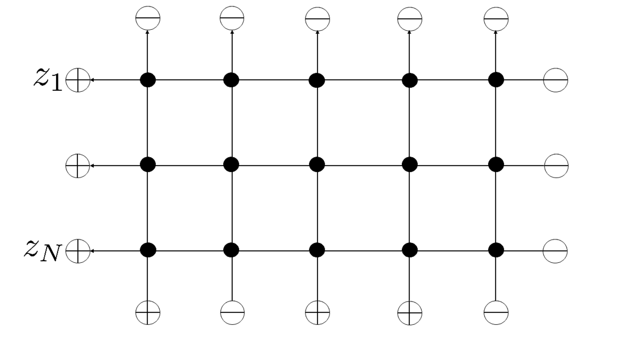
The dual wavefunction ⟨Φ(z1,…,zN)|x1¯⋯xN¯⟩\langle\Phi(z_{1},\dots,z_{N})|\overline{x_{1}}\cdots\overline{x_{N}}\rangle is defined as the overlap between the arbitrary dual NN-hole state ⟨Φ⁡(z1,…,zN)|\langle\Phi(z_{1},\dots,z_{N})| and hole configurations |x1¯⋯xN¯⟩|\overline{x_{1}}\cdots\overline{x_{N}}\rangle (see Figure 3 for an example of a graphical description of the dual wavefunction).
Refer to caption
Figure 3: The dual wavefunction ⟨Φ(z1,…,zN)|x1¯⋯xN¯⟩\langle\Phi(z_{1},\dots,z_{N})|\overline{x_{1}}\cdots\overline{x_{N}}\rangle for the case M=5M=5, N=3N=3, (x1¯,x2¯,x3¯)=(2,3,5)(\overline{x_{1}},\overline{x_{2}},\overline{x_{3}})=(2,3,5).

We show the following relation between the dual wavefunction and the Schur polynomials.

Theorem 4.1.

The dual wavefunction ⟨Φ(z1,…,zN)|x1¯⋯xN¯⟩\langle\Phi(z_{1},\dots,z_{N})|\overline{x_{1}}\cdots\overline{x_{N}}\rangle can be expressed by the Schur polynomials as

⟨Φ(z1,…,zN)|x1¯⋯xN¯⟩=tN⁡(M−N)∏1≤j<k≤N(zj+tzk)sλ¯({zt}N).\displaystyle\langle\Phi(z_{1},\dots,z_{N})|\overline{x_{1}}\cdots\overline{x_{N}}\rangle=t^{N(M-N)}\prod_{1\leq j<k\leq N}(z_{j}+tz_{k})s_{\overline{\lambda}}\Bigg(\Bigg\{\frac{z}{t}\Bigg\}_{N}\Bigg). (4.3)

Here the Young diagram for the Schur polynomials correspond to the particle configuration under the relation λj¯=xN−j+1¯−N+j−1\overline{\lambda_{j}}=\overline{x_{N-j+1}}-N+j-1, j=1,…,Nj=1,\dots,N, and the symmetric variables are {zt}N={z1t,…,zNt}\displaystyle\Bigg\{\frac{z}{t}\Bigg\}_{N}=\Bigg\{\frac{z_{1}}{t},\dots,\frac{z_{N}}{t}\Bigg\}.

Before proving Theorem 4.1, let us make some comments. There is a factor tN⁡(M−N)t^{N(M-N)} which depends on the number of sites MM and the number of particles NN in the right hand side of (4.3). What makes things more complicated is that the symmetric variables of the Schur polynomials are {zt}N\displaystyle\Bigg\{\frac{z}{t}\Bigg\}_{N}, which are the reasons why the relation for the dual wavefunction (4.3) seems hard to find. We actually first found this Theorem by using the statistical physical method given in the next section. One advantages of the proof given in this section following [13] is that the proof naturally lifts to the correspondence between a generalization of the Felderhof model and the factorial Schur polynoimals.

Proof.

We rewrite (4.3) by rescaling each zjz_{j} to t​zjtz_{j} (4.3) in the following form

tN⟨1⋯M|(B⁡(t​z1)tM)⋯(B⁡(t​zN)tM)|x1¯⋯xN¯⟩=∏1≤j<k≤N(1tzj+zk)sλ¯({z}N).\displaystyle t^{N}\langle 1\cdots M|\Bigg(\frac{B(tz_{1})}{t^{M}}\Bigg)\cdots\Bigg(\frac{B(tz_{N})}{t^{M}}\Bigg)|\overline{x_{1}}\cdots\overline{x_{N}}\rangle=\prod_{1\leq j<k\leq N}\Bigg(\frac{1}{t}z_{j}+z_{k}\Bigg)s_{\overline{\lambda}}(\{z\}_{N}). (4.4)

For giving a proof, it is convenient to introduce the rescaled LL-operator

L~​(z,t)=1t​L​(t​z,t)=(1/t000011/t00(t+1)​zz0000z),\displaystyle\widetilde{L}(z,t)=\frac{1}{t}L(tz,t)=\left(\begin{array}[]{cccc}1/t&0&0&0\\ 0&1&1/t&0\\ 0&(t+1)z&z&0\\ 0&0&0&z\end{array}\right),

and the rescaled monodromy matrix

T~a(z)=L~a​M(z,t)⋯L~a​1(z,t)=(A~​(z)B~​(z)C~​(z)D~​(z))a.\displaystyle\widetilde{T}_{a}(z)=\widetilde{L}_{aM}(z,t)\cdots\widetilde{L}_{a1}(z,t)=\begin{pmatrix}\widetilde{A}(z)&\widetilde{B}(z)\\ \widetilde{C}(z)&\widetilde{D}(z)\end{pmatrix}_{a}. (4.10)

Using these rescaled objects, (4.4) can be expressed as

tN⟨1⋯M|B~(z1)⋯B~(zN)|x1¯⋯xN¯⟩=∏1≤j<k≤N(1tzj+zk)sλ¯({z}N).\displaystyle t^{N}\langle 1\cdots M|\widetilde{B}(z_{1})\cdots\widetilde{B}(z_{N})|\overline{x_{1}}\cdots\overline{x_{N}}\rangle=\prod_{1\leq j<k\leq N}\Bigg(\frac{1}{t}z_{j}+z_{k}\Bigg)s_{\overline{\lambda}}(\{z\}_{N}). (4.11)

Instead of proving (4.3), we show (4.11) since this is equivalent to (4.3) and is the expression which one can use the argument given in [13].

We first show the following lemma.

Lemma 4.2.
∏1≤j<k≤N(1tzj+zk)−1tN⟨1⋯M|B~(z1)⋯B~(zN)|x1¯⋯xN¯⟩,\displaystyle\prod_{1\leq j<k\leq N}\Bigg(\frac{1}{t}z_{j}+z_{k}\Bigg)^{-1}t^{N}\langle 1\cdots M|\widetilde{B}(z_{1})\cdots\widetilde{B}(z_{N})|\overline{x_{1}}\cdots\overline{x_{N}}\rangle, (4.12)

does not depend on tt.

Proof.

We prove this lemma by showing the following properties for
tN⟨1⋯M|B~(z1)⋯B~(zN)|x1¯⋯xN¯⟩t^{N}\langle 1\cdots M|\widetilde{B}(z_{1})\cdots\widetilde{B}(z_{N})|\overline{x_{1}}\cdots\overline{x_{N}}\rangle:

  1. 1.

    tN⟨1⋯M|B~(z1)⋯B~(zN)|x1¯⋯xN¯⟩t^{N}\langle 1\cdots M|\widetilde{B}(z_{1})\cdots\widetilde{B}(z_{N})|\overline{x_{1}}\cdots\overline{x_{N}}\rangle is a polynomial of t′:=t−1t^{\prime}:=t^{-1} with highest degree N⁡(N−1)/2N(N-1)/2.

  2. 2.

    tN⟨1⋯M|B~(z1)⋯B~(zN)|x1¯⋯xN¯⟩t^{N}\langle 1\cdots M|\widetilde{B}(z_{1})\cdots\widetilde{B}(z_{N})|\overline{x_{1}}\cdots\overline{x_{N}}\rangle has t′​zj+zkt^{\prime}z_{j}+z_{k}, 1≤j<k≤N1\leq j<k\leq N as factors.

We first show degt′(tN⟨1⋯M|B~(z1)⋯B~(zN)|x1¯⋯xN¯⟩)≤N(N−1)/2\mathrm{deg}_{t^{\prime}}(t^{N}\langle 1\cdots M|\widetilde{B}(z_{1})\cdots\widetilde{B}(z_{N})|\overline{x_{1}}\cdots\overline{x_{N}}\rangle)\leq N(N-1)/2 by induction on NN. The case N=1N=1 follows as an special case of the general fact
0≤degt′(t⟨x1¯⋯xN¯|B~(z)|y1¯⋯yN+1¯⟩)≤N0\leq\mathrm{deg}_{t^{\prime}}(t\langle\overline{x_{1}}\cdots\overline{x_{N}}|\widetilde{B}(z)|\overline{y_{1}}\cdots\overline{y_{N+1}}\rangle)\leq N which can be seen easily from the definition of the rescaled LL-operator L~​(z,t)\widetilde{L}(z,t). Next, let us assume degt′(tN⟨1⋯M|B~(z1)⋯B~(zN)|x1¯⋯xN¯⟩)≤N(N−1)/2\mathrm{deg}_{t^{\prime}}(t^{N}\langle 1\cdots M|\widetilde{B}(z_{1})\cdots\widetilde{B}(z_{N})|\overline{x_{1}}\cdots\overline{x_{N}}\rangle)\leq N(N-1)/2. One can see degt′(tN+1⟨1⋯M|B~(z1)⋯B~(zN+1)|y1¯⋯yN+1¯⟩)≤(N+1)N/2\mathrm{deg}_{t^{\prime}}(t^{N+1}\langle 1\cdots M|\widetilde{B}(z_{1})\cdots\widetilde{B}(z_{N+1})|\overline{y_{1}}\cdots\overline{y_{N+1}}\rangle)\leq(N+1)N/2 by combining the assumption degt′(tN⟨1⋯M|B~(z1)⋯B~(zN)|x1¯⋯xN¯⟩)≤N(N−1)/2\mathrm{deg}_{t^{\prime}}(t^{N}\langle 1\cdots M|\widetilde{B}(z_{1})\cdots\widetilde{B}(z_{N})|\overline{x_{1}}\cdots\overline{x_{N}}\rangle)\leq N(N-1)/2,
the fact 0≤degt′(t⟨x1¯⋯xN¯|B~(z)|y1¯⋯yN+1¯⟩)≤N0\leq\mathrm{deg}_{t^{\prime}}(t\langle\overline{x_{1}}\cdots\overline{x_{N}}|\widetilde{B}(z)|\overline{y_{1}}\cdots\overline{y_{N+1}}\rangle)\leq N and the decomposition

tN+1⟨1⋯M|B~(z1)⋯B~(zN+1)|y1¯⋯yN+1¯⟩\displaystyle t^{N+1}\langle 1\cdots M|\widetilde{B}(z_{1})\cdots\widetilde{B}(z_{N+1})|\overline{y_{1}}\cdots\overline{y_{N+1}}\rangle
=\displaystyle= ∑{x¯}(tN⟨1⋯M|B~(z1)⋯B~(zN)|x1¯⋯xN¯⟩)(t⟨x1¯⋯xN¯|B~(zN+1)|y1¯⋯yN+1¯⟩).\displaystyle\sum_{\{\overline{x}\}}(t^{N}\langle 1\cdots M|\widetilde{B}(z_{1})\cdots\widetilde{B}(z_{N})|\overline{x_{1}}\cdots\overline{x_{N}}\rangle)(t\langle\overline{x_{1}}\cdots\overline{x_{N}}|\widetilde{B}(z_{N+1})|\overline{y_{1}}\cdots\overline{y_{N+1}}\rangle). (4.13)

Next we show Property 2. The commutation relation (2.26) can be rewritten as the following commutation relation between the rescaled BB-operators

(z1+t′​z2)​B~​(z1)​B~​(z2)=B~​(z2)​B~​(z1)​(t′​z1+z2).\displaystyle(z_{1}+t^{\prime}z_{2})\widetilde{B}(z_{1})\widetilde{B}(z_{2})=\widetilde{B}(z_{2})\widetilde{B}(z_{1})(t^{\prime}z_{1}+z_{2}). (4.14)

Applying the commutation relation (4.14) repeatedly, one gets the following equality

tN⟨1⋯M|B~(z1)⋯B~(zN)|x1¯⋯xN¯⟩∏1≤j<k≤N(zj+t′zk)\displaystyle t^{N}\langle 1\cdots M|\widetilde{B}(z_{1})\cdots\widetilde{B}(z_{N})|\overline{x_{1}}\cdots\overline{x_{N}}\rangle\prod_{1\leq j<k\leq N}(z_{j}+t^{\prime}z_{k})
=\displaystyle= tN⟨1⋯M|B~(zN)⋯B~(z1)|x1¯⋯xN¯⟩∏1≤j<k≤N(t′zj+zk).\displaystyle t^{N}\langle 1\cdots M|\widetilde{B}(z_{N})\cdots\widetilde{B}(z_{1})|\overline{x_{1}}\cdots\overline{x_{N}}\rangle\prod_{1\leq j<k\leq N}(t^{\prime}z_{j}+z_{k}). (4.15)

Note that in the equality (4.15), the factors tN⟨1⋯M|B~(z1)⋯B~(zN)|x1¯⋯xN¯⟩t^{N}\langle 1\cdots M|\widetilde{B}(z_{1})\cdots\widetilde{B}(z_{N})|\overline{x_{1}}\cdots\overline{x_{N}}\rangle,
∏1≤j<k≤N(zj+t′​zk)\prod_{1\leq j<k\leq N}(z_{j}+t^{\prime}z_{k}), tN⟨1⋯M|B~(zN)⋯B~(z1)|x1¯⋯xN¯⟩t^{N}\langle 1\cdots M|\widetilde{B}(z_{N})\cdots\widetilde{B}(z_{1})|\overline{x_{1}}\cdots\overline{x_{N}}\rangle and ∏1≤j<k≤N(t′​zj+zk)\prod_{1\leq j<k\leq N}(t^{\prime}z_{j}+z_{k}) are polynomials of t′t^{\prime}. From this fact and that ∏1≤j<k≤N(zj+t′​zk)\prod_{1\leq j<k\leq N}(z_{j}+t^{\prime}z_{k}) is not divided by ∏1≤j<k≤N(t′​zj+zk)\prod_{1\leq j<k\leq N}(t^{\prime}z_{j}+z_{k}), one can see tN⟨1⋯M|B~(z1)⋯B~(zN)|x1¯⋯xN¯⟩t^{N}\langle 1\cdots M|\widetilde{B}(z_{1})\cdots\widetilde{B}(z_{N})|\overline{x_{1}}\cdots\overline{x_{N}}\rangle is divided by ∏1≤j<k≤N(t′​zj+zk)\prod_{1\leq j<k\leq N}(t^{\prime}z_{j}+z_{k}).

From Property 2, we have degt′(tN⟨1⋯M|B~(z1)⋯B~(zN)|x1¯⋯xN¯⟩)≥N(N−1)/2\mathrm{deg}_{t^{\prime}}(t^{N}\langle 1\cdots M|\widetilde{B}(z_{1})\cdots\widetilde{B}(z_{N})|\overline{x_{1}}\cdots\overline{x_{N}}\rangle)\geq N(N-1)/2. Together with degt′(tN⟨1⋯M|B~(z1)⋯B~(zN)|x1¯⋯xN¯⟩)≤N(N−1)/2\mathrm{deg}_{t^{\prime}}(t^{N}\langle 1\cdots M|\widetilde{B}(z_{1})\cdots\widetilde{B}(z_{N})|\overline{x_{1}}\cdots\overline{x_{N}}\rangle)\leq N(N-1)/2 which is proved before, we have Property 1.

∎

From Lemma 4.2, one sees that to study the wavefunction, it is enough to examine a particular value of tt. The case when t=−1t=-1 in which the six-vertex model reduces to a five-vertex model

L~​(z,−1)=−L⁡(−z,−1)=(−100001−1000z0000z),\displaystyle\widetilde{L}(z,-1)=-L(-z,-1)=\left(\begin{array}[]{cccc}-1&0&0&0\\ 0&1&-1&0\\ 0&0&z&0\\ 0&0&0&z\end{array}\right),

is easy to examine, and we have the following relation.

Lemma 4.3.

We have

∏1≤j<k≤N(1tzj+zk)−1tN⟨1⋯M|B~(z1)⋯B~(zN)|x1¯⋯xN¯⟩|t=−1=sλ¯({z}N).\displaystyle\prod_{1\leq j<k\leq N}\Bigg(\frac{1}{t}z_{j}+z_{k}\Bigg)^{-1}t^{N}\langle 1\cdots M|\widetilde{B}(z_{1})\cdots\widetilde{B}(z_{N})|\overline{x_{1}}\cdots\overline{x_{N}}\rangle\Bigg|_{t=-1}=s_{\overline{\lambda}}(\{z\}_{N}). (4.21)
Proof.

To prove the Lemma is equivalent to show

⟨1⋯M|B~(z1)⋯B~(zN)|x1¯⋯xN¯⟩|t=−1=(−1)N∏1≤j<k≤N(−zj+zk)sλ¯({z}N).\displaystyle\langle 1\cdots M|\widetilde{B}(z_{1})\cdots\widetilde{B}(z_{N})|\overline{x_{1}}\cdots\overline{x_{N}}\rangle|_{t=-1}=(-1)^{N}\prod_{1\leq j<k\leq N}(-z_{j}+z_{k})s_{\overline{\lambda}}(\{z\}_{N}). (4.22)

To show this, we first note that the matrix elements of a single BB-operator is given by

⟨x1¯⋯xk−1¯|B~(z)|y1¯⋯yk¯⟩=\displaystyle\langle\overline{x_{1}}\cdots\overline{x_{k-1}}|\widetilde{B}(z)|\overline{y_{1}}\cdots\overline{y_{k}}\rangle= (−1)k​(−1)j−1​zyj¯−1,\displaystyle(-1)^{k}(-1)^{j-1}z^{\overline{y_{j}}-1}, (4.23)

when the hole configurations {x¯}\{\overline{x}\} and {y¯}\{\overline{y}\} satisfy
x1¯=y1¯,⋯,xj−1¯=yj−1¯\overline{x_{1}}=\overline{y_{1}},\cdots,\overline{x_{j-1}}=\overline{y_{j-1}}, xj¯=yj+1¯,⋯,xk−1¯=yk¯\overline{x_{j}}=\overline{y_{j+1}},\cdots,\overline{x_{k-1}}=\overline{y_{k}} for some jj, and 0 otherwise.

Since the matrix elements of a single BB-operator are essentially the same with the ones for the original wavefunction at t=−1t=-1 in [13] except the sign (−1)k(-1)^{k} (we also have to translate the hole configurations to particle configurations), the same argument can be appplied. One observes that the number of the inner states whose weights gives non-zero contributions to the dual wavefunction is N!N!. The weight of each nonvanishing inner state corresponds to one term (−1)σ​∏j=1Nzjλσ​(j)¯+N−σ⁡(j)(-1)^{\sigma}\prod_{j=1}^{N}z_{j}^{\overline{\lambda_{\sigma}(j)}+N-\sigma(j)} of the determinant expansion of the numerator (3.1) of the Schur polynomials multipled by the extra factor (−1)N⁡(N+1)/2(-1)^{N(N+1)/2}. The factor (−1)N⁡(N+1)/2(-1)^{N(N+1)/2} appears since the dual wavefunction is constructed from NN layers of BB-operators, and the kk-th layer of the BB-operator has the extra sign (−1)k(-1)^{k} in the right hand side of (4.23), hence the total contribution of NN layers of the BB operators gives the extra sign ∏k=1N(−1)k=(−1)N⁡(N+1)/2\prod_{k=1}^{N}(-1)^{k}=(-1)^{N(N+1)/2}. We further rewrite the extra factor (−1)N⁡(N+1)/2(-1)^{N(N+1)/2} as

(−1)N⁡(N+1)/2=(−1)N​(−1)N⁡(N−1)/2=(−1)N​∏1≤j<k≤N(−zj+zk)∏1≤j<k≤N(zj−zk),\displaystyle(-1)^{N(N+1)/2}=(-1)^{N}(-1)^{N(N-1)/2}=(-1)^{N}\frac{\prod_{1\leq j<k\leq N}(-z_{j}+z_{k})}{\prod_{1\leq j<k\leq N}(z_{j}-z_{k})}, (4.24)

to get

⟨1⋯M|B~(z1)⋯B~(zN)|x1¯⋯xN¯⟩|t=−1\displaystyle\langle 1\cdots M|\widetilde{B}(z_{1})\cdots\widetilde{B}(z_{N})|\overline{x_{1}}\cdots\overline{x_{N}}\rangle|_{t=-1}
=\displaystyle= (−1)N⁡(N+1)/2​∑σ∈SN(−1)σ​∏j=1Nzjλσ​(j)¯+N−σ⁡(j)\displaystyle(-1)^{N(N+1)/2}\sum_{\sigma\in S_{N}}(-1)^{\sigma}\prod_{j=1}^{N}z_{j}^{\overline{\lambda_{\sigma}(j)}+N-\sigma(j)}
=\displaystyle= (−1)N​∏1≤j<k≤N(−zj+zk)∏1≤j<k≤N(zj−zk)​∑σ∈SN(−1)σ​∏j=1Nzjλσ​(j)¯+N−σ⁡(j)\displaystyle(-1)^{N}\frac{\prod_{1\leq j<k\leq N}(-z_{j}+z_{k})}{\prod_{1\leq j<k\leq N}(z_{j}-z_{k})}\sum_{\sigma\in S_{N}}(-1)^{\sigma}\prod_{j=1}^{N}z_{j}^{\overline{\lambda_{\sigma}(j)}+N-\sigma(j)}
=\displaystyle= (−1)N​∏1≤j<k≤N(−zj+zk)​sλ¯​({z}N).\displaystyle(-1)^{N}\prod_{1\leq j<k\leq N}(-z_{j}+z_{k})s_{\overline{\lambda}}(\{z\}_{N}). (4.25)

∎

From Lemma 4.2 and (4.21), we have

∏1≤j<k≤N(1tzj+zk)−1tN⟨1⋯M|B~(z1)⋯B~(zN)|x1¯⋯xN¯⟩\displaystyle\prod_{1\leq j<k\leq N}\Bigg(\frac{1}{t}z_{j}+z_{k}\Bigg)^{-1}t^{N}\langle 1\cdots M|\widetilde{B}(z_{1})\cdots\widetilde{B}(z_{N})|\overline{x_{1}}\cdots\overline{x_{N}}\rangle
=\displaystyle= ∏1≤j<k≤N(1tzj+zk)−1tN⟨1⋯M|B~(z1)⋯B~(zN)|x1¯⋯xN¯⟩|t=−1\displaystyle\prod_{1\leq j<k\leq N}\Bigg(\frac{1}{t}z_{j}+z_{k}\Bigg)^{-1}t^{N}\langle 1\cdots M|\widetilde{B}(z_{1})\cdots\widetilde{B}(z_{N})|\overline{x_{1}}\cdots\overline{x_{N}}\rangle\Bigg|_{t=-1}
=\displaystyle= sλ¯​({z}N),\displaystyle s_{\overline{\lambda}}(\{z\}_{N}), (4.26)

which is exactly (4.11), hence Theorem 4.1 is proved. ∎

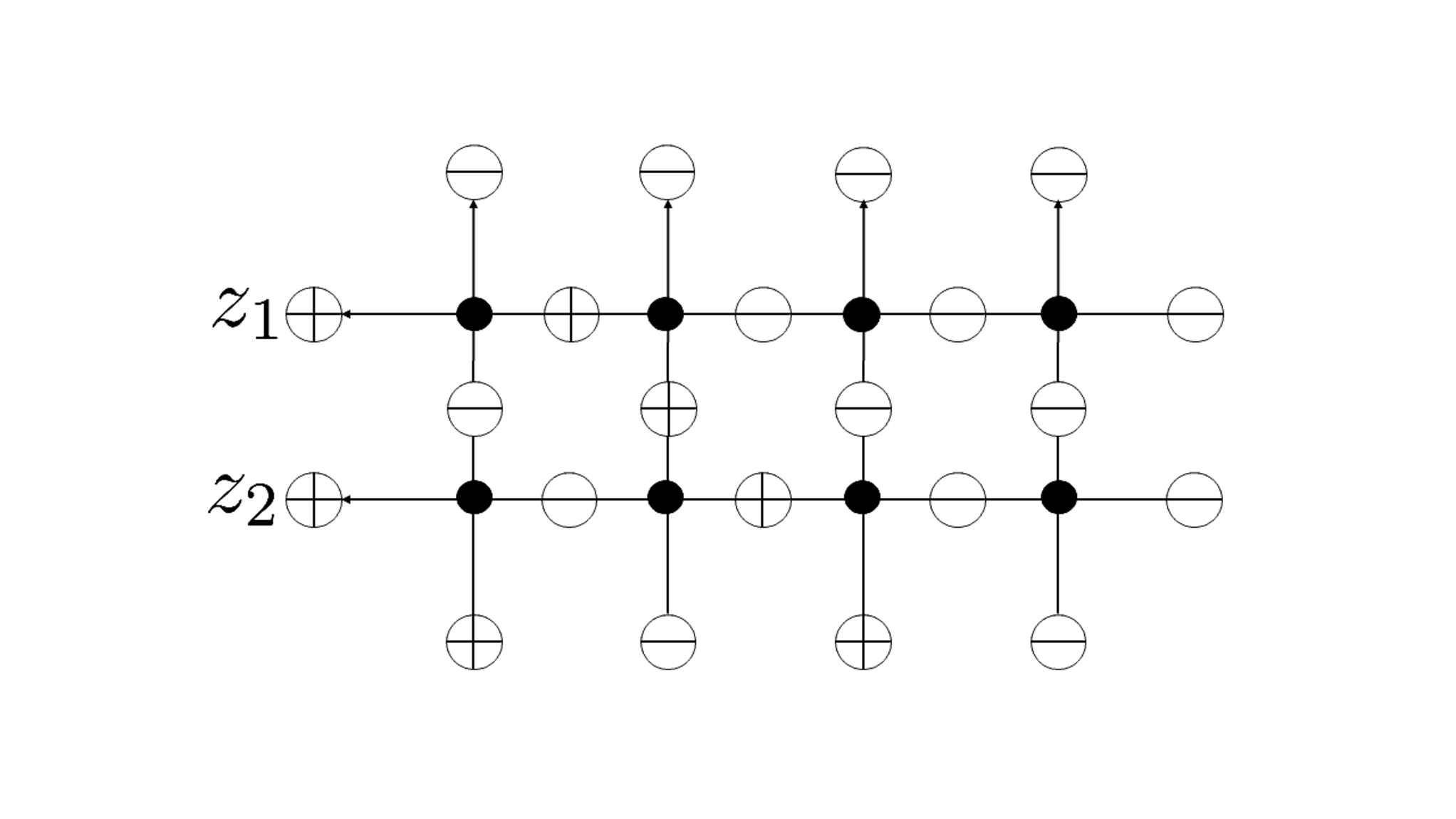
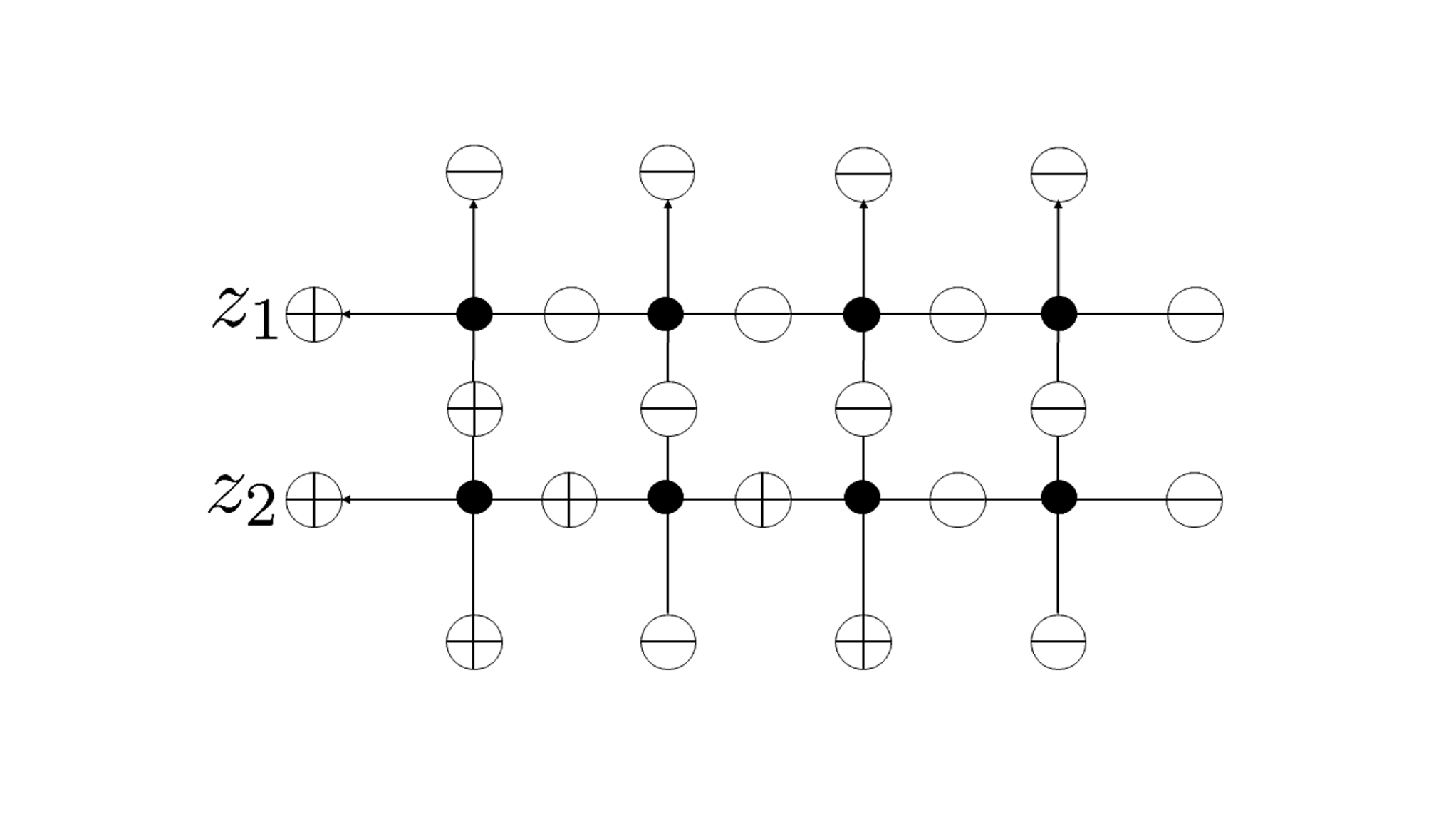
Example Let us check Theorem 4.1 by an example M=4M=4, N=2N=2 , (x1¯,x2¯)=(2,4)(\overline{x_{1}},\overline{x_{2}})=(2,4). The corresponding Young diagram is λ¯=(λ¯1,λ2¯)=(x2¯−2,x1¯−1)=(4−2,2−1)=(2,1)\overline{\lambda}=(\overline{\lambda}_{1},\overline{\lambda_{2}})=(\overline{x_{2}}-2,\overline{x_{1}}-1)=(4-2,2-1)=(2,1). The left hand side of (4.3) can be calculated graphically by noting that there are three inner states whose weights make nonzero contributions to the dual wavefunction ⟨Φ(z1,z2)|x1¯=2,x2¯=4⟩\langle\Phi(z_{1},z_{2})|\overline{x_{1}}=2,\overline{x_{2}}=4\rangle, which are given in Figures 4, 5 and 6. From its graphical description and using the data of the matrix elements of the LL-operator (2) and multiplying them, one sees that each of the configurations have weights t2​z1​z23t^{2}z_{1}z_{2}^{3}, t⁡(t+1)​z12​z22t(t+1)z_{1}^{2}z_{2}^{2} and t​z13​z2tz_{1}^{3}z_{2}. Summing up the weights and noting that one can extract (z1+t​z2)(z_{1}+tz_{2}) as an overall factor, we have

t2​z1​z23+t⁡(t+1)​z12​z22+t​z13​z2\displaystyle t^{2}z_{1}z_{2}^{3}+t(t+1)z_{1}^{2}z_{2}^{2}+tz_{1}^{3}z_{2} =t4​(z1+t​z2)​((z1t)2​(z2t)+(z1t)​(z2t)2)\displaystyle=t^{4}(z_{1}+tz_{2})\Bigg(\Bigg(\frac{z_{1}}{t}\Bigg)^{2}\Bigg(\frac{z_{2}}{t}\Bigg)+\Bigg(\frac{z_{1}}{t}\Bigg)\Bigg(\frac{z_{2}}{t}\Bigg)^{2}\Bigg)
=t4​(z1+t​z2)​s(2,1)​(z1t,z2t),\displaystyle=t^{4}(z_{1}+tz_{2})s_{(2,1)}\Bigg(\frac{z_{1}}{t},\frac{z_{2}}{t}\Bigg), (4.27)

which is nothing but the right hand side of (4.3).
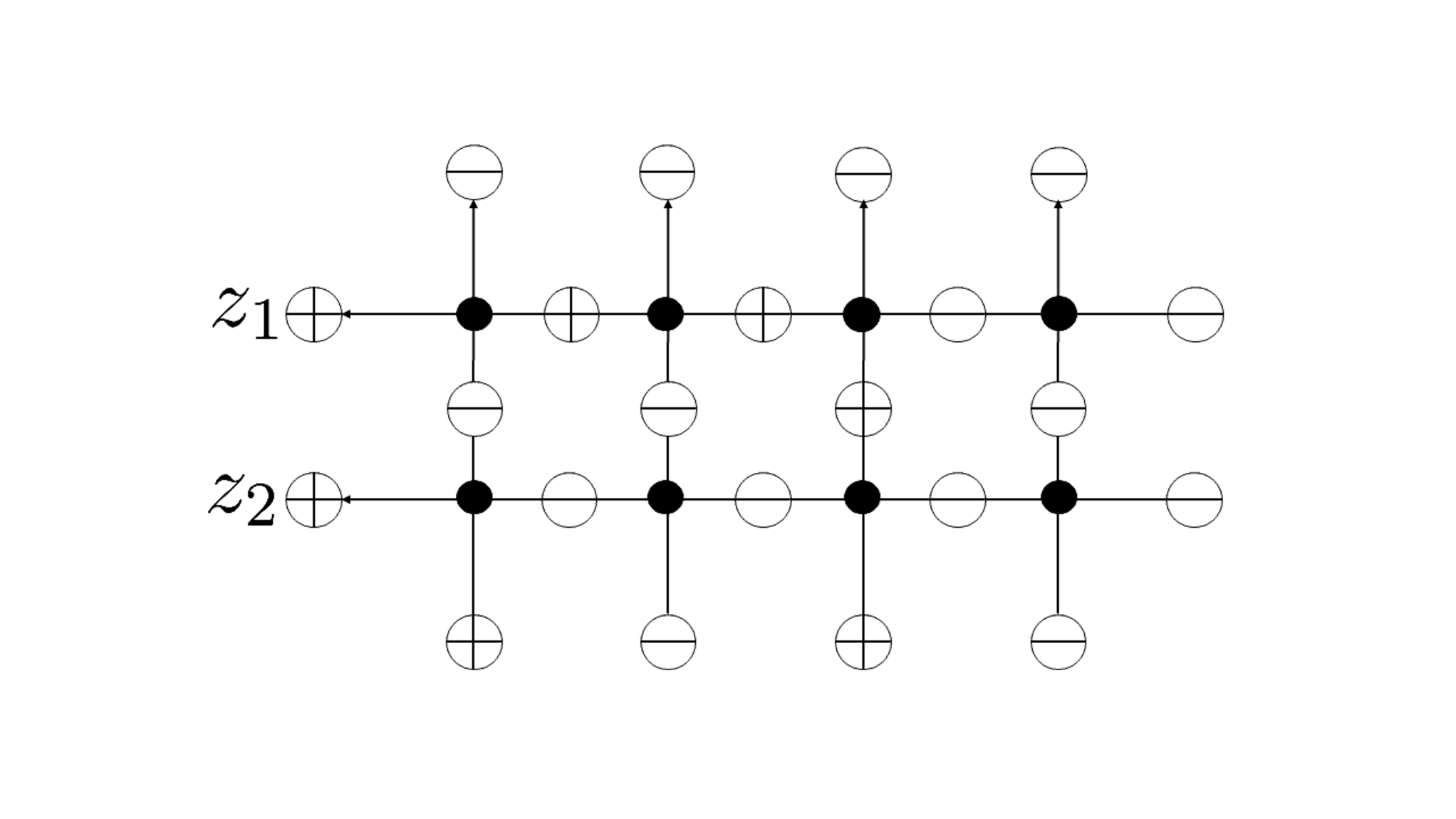
Refer to caption
Figure 4: An inner state of the dual wavefunction ⟨Φ(z1,z2)|x1¯=2,x2¯=4⟩\langle\Phi(z_{1},z_{2})|\overline{x_{1}}=2,\overline{x_{2}}=4\rangle giving the weight t2​z1​z23t^{2}z_{1}z_{2}^{3}.
Refer to caption
Figure 5: An inner state of the dual wavefunction ⟨Φ(z1,z2)|x1¯=2,x2¯=4⟩\langle\Phi(z_{1},z_{2})|\overline{x_{1}}=2,\overline{x_{2}}=4\rangle giving the weight t⁡(t+1)​z12​z22t(t+1)z_{1}^{2}z_{2}^{2}.
Refer to caption
Figure 6: An inner state of the dual wavefunction ⟨Φ(z1,z2)|x1¯=2,x2¯=4⟩\langle\Phi(z_{1},z_{2})|\overline{x_{1}}=2,\overline{x_{2}}=4\rangle giving the weight t​z13​z2tz_{1}^{3}z_{2}.

5 Another proof

We give another proof of Theorem 4.1 by using a modern statistical mechanical method and an analysis on a fundamental object in quantum integrable models, i.e., we use the matrix product method and the domain wall boundary partition function, as was done in the case of the Grothendieck polynomials in [21] (see also [22] in which we demonstrate a proof of Theorem 3.2 by using the same arguments given in this section). We prove Theorem 4.1 as follows. We first rewrite the dual wavefunction into a matrix product form, following [17, 18]. The matrix product form can be expressed as a determinant with some overall factor which remains to be calculated. The information of the hole configuration {x1¯,x2¯,…,xN¯}\{\overline{x_{1}},\overline{x_{2}},\dots,\overline{x_{N}}\} is encoded in the determinant. On the other hand, the overall factor is independent of the hole positions, and this factor can be determined by considering the specific configuration: we explicitly evaluate the overlap of the consecutive hole configuration (i.e. xj¯=j\overline{x_{j}}=j) whose evaluation essentially reduces to that of the domain wall boundary partition function.

Proof.

Let us begin to compute the wavefunction ⟨Φ({z}N)|x1¯⋯xN¯⟩\langle\Phi(\{z\}_{N})|\overline{x_{1}}\cdots\overline{x_{N}}\rangle. We first rewrite it into the matrix product representation. With the help of graphical description, one finds that the wavefunction can be written as

⟨Φ({z}N)|x1¯⋯xN¯⟩=TrW⊗N[⟨1⋯M|∏a=1NTa(za)|x1¯⋯xN¯⟩P],\displaystyle\langle\Phi(\{z\}_{N})|\overline{x_{1}}\cdots\overline{x_{N}}\rangle=\Tr_{W^{\otimes N}}\left[\langle 1\cdots M|\prod_{a=1}^{N}T_{a}(z_{a})|\overline{x_{1}}\cdots\overline{x_{N}}\rangle P\right], (5.1)

where P=|1N⟩​⟨0N|P=|1^{N}\rangle\langle 0^{N}| is an operator acting on the tensor product of auxiliary spaces W1⊗⋯⊗WNW_{1}\otimes\dots\otimes W_{N}. The trace here is also over the auxiliary spaces.

Changing the viewpoint of the products of the monodromy matrices, we have

∏a=1NTa​(za)=∏j=1M𝒯j​({z}N),\displaystyle\prod_{a=1}^{N}T_{a}(z_{a})=\prod_{j=1}^{M}\mathcal{T}_{j}(\{z\}_{N}), (5.2)

where 𝒯j​({z}N):=∏a=1NLa​j​(za)∈End⁡(W⊗N⊗Vj)\mathcal{T}_{j}(\{z\}_{N}):=\prod_{a=1}^{N}L_{aj}(z_{a})\in\End(W^{\otimes N}\otimes V_{j}) can be regarded as a monodromy matrix consisting of LL-operators acting on the same quantum space VjV_{j} (but acting on different auxiliary spaces). The monodromy matrix is decomposed as

𝒯j​({z}N)\displaystyle\mathcal{T}_{j}(\{z\}_{N}) :=(𝒜N​({z}N)ℬN​({z}N)𝒞N​({z}N)𝒟N​({z}N))j,\displaystyle:=\begin{pmatrix}\mathcal{A}_{N}(\{z\}_{N})&\mathcal{B}_{N}(\{z\}_{N})\\ \mathcal{C}_{N}(\{z\}_{N})&\mathcal{D}_{N}(\{z\}_{N})\end{pmatrix}_{j}, (5.3)

where the elements (𝒜N\mathcal{A}_{N}, etc.) act on W1⊗⋯⊗WNW_{1}\otimes\dots\otimes W_{N}.

The wavefunction (5.1) can then be rewritten by 𝒯j​({z}N)\mathcal{T}_{j}(\{z\}_{N}) as

⟨Φ({z}N)|x1¯⋯xN¯⟩\displaystyle\langle\Phi(\{z\}_{N})|\overline{x_{1}}\cdots\overline{x_{N}}\rangle =TrW⊗N[⟨1⋯M|∏j=1M𝒯j({z}N)|x1¯⋯xN¯⟩P]\displaystyle=\Tr_{W^{\otimes N}}\left[\langle 1\cdots M|\prod_{j=1}^{M}\mathcal{T}_{j}(\{z\}_{N})|\overline{x_{1}}\cdots\overline{x_{N}}\rangle P\right]
=TrW⊗N⁡[𝒟NM−xN¯​𝒞N​𝒟NxN¯−xN−1¯−1​…​𝒞N​𝒟Nx2¯−x1¯−1​𝒞N​𝒟Nx1¯−1​P].\displaystyle=\Tr_{W^{\otimes N}}\left[\mathcal{D}_{N}^{M-\overline{x_{N}}}\mathcal{C}_{N}\mathcal{D}_{N}^{\overline{x_{N}}-\overline{x_{N-1}}-1}\dots\mathcal{C}_{N}\mathcal{D}_{N}^{\overline{x_{2}}-\overline{x_{1}}-1}\mathcal{C}_{N}\mathcal{D}_{N}^{\overline{x_{1}}-1}P\right]. (5.4)

For these operators, one finds the following recursive relations:

𝒟n+1​({z}n+1)=𝒟n​({z}n)⊗(t00zn+1)+𝒞n​({z}n)⊗(00(1+t)​zn+10),\displaystyle\mathcal{D}_{n+1}(\{z\}_{n+1})=\mathcal{D}_{n}(\{z\}_{n})\otimes\begin{pmatrix}t&0\\ 0&z_{n+1}\end{pmatrix}+\mathcal{C}_{n}(\{z\}_{n})\otimes\begin{pmatrix}0&0\\ (1+t)z_{n+1}&0\end{pmatrix}, (5.5)
𝒞n+1​({z}n+1)=𝒟n​({z}n)⊗(0100)+𝒞n​({z}n)⊗(100zn+1),\displaystyle\mathcal{C}_{n+1}(\{z\}_{n+1})=\mathcal{D}_{n}(\{z\}_{n})\otimes\begin{pmatrix}0&1\\ 0&0\end{pmatrix}+\mathcal{C}_{n}(\{z\}_{n})\otimes\begin{pmatrix}1&0\\ 0&z_{n+1}\end{pmatrix}, (5.6)

with the initial condition

𝒟1=(t00z1),𝒞1=(0100).\displaystyle\mathcal{D}_{1}=\begin{pmatrix}t&0\\ 0&z_{1}\end{pmatrix},\quad\mathcal{C}_{1}=\begin{pmatrix}0&1\\ 0&0\end{pmatrix}. (5.7)

By using the recursive relations (5.5) and (5.6), one sees that these operators satisfy the following simple algebra.

Lemma 5.1.

There exists a decomposition of 𝒞n\mathcal{C}_{n} : 𝒞n=∑j=1n𝒞n(j)\mathcal{C}_{n}=\sum_{j=1}^{n}\mathcal{C}_{n}^{(j)} such that the following algebraic relations hold for 𝒟n\mathcal{D}_{n} and 𝒞n(j)\mathcal{C}_{n}^{(j)}:

𝒞n(j)​𝒟n=zjt​𝒟n​𝒞n(j),\displaystyle\mathcal{C}_{n}^{(j)}\mathcal{D}_{n}=\frac{z_{j}}{t}\mathcal{D}_{n}\mathcal{C}_{n}^{(j)}, (5.8)
(𝒞n(j))2=0,\displaystyle(\mathcal{C}_{n}^{(j)})^{2}=0, (5.9)
𝒞n(j)​𝒞n(k)=−zjzk​𝒞n(k)​𝒞n(j),(j≠k).\displaystyle\mathcal{C}_{n}^{(j)}\mathcal{C}_{n}^{(k)}=-\frac{z_{j}}{z_{k}}\mathcal{C}_{n}^{(k)}\mathcal{C}_{n}^{(j)},\ \ \ (j\neq k). (5.10)
Proof.

We show by induction on nn. For n=1n=1, from (5.7) 𝒟1\mathcal{D}_{1} is diagonal and one can directly see that the relations are satisfied. For nn, we assume that 𝒟n\mathcal{D}_{n} is diagonalizable and write the corresponding diagonal matrix as 𝒟n=Gn−1​𝒟n​Gn\mathscr{D}_{n}=G_{n}^{-1}\mathcal{D}_{n}G_{n}. Also writing 𝒞n=Gn−1​𝒞n​Gn\mathscr{C}_{n}=G_{n}^{-1}\mathcal{C}_{n}G_{n} and 𝒞n=∑j=1n𝒞n(j)\mathscr{C}_{n}=\sum_{j=1}^{n}\mathscr{C}_{n}^{(j)}, and noting that the algebraic relations above do not depend on the choice of basis, we suppose by the induction hypothesis that the same relations are satisfied by 𝒟n\mathscr{D}_{n} and 𝒞n(j)\mathscr{C}_{n}^{(j)}.

We show that the relations hold for n+1n+1. To this end, we first construct Gn+1G_{n+1}. Noting from (5.5) that 𝒟n+1\mathcal{D}_{n+1} is an upper triangular block matrix whose block diagonal elements are written in terms of 𝒟n\mathcal{D}_{n}, we assume that Gn+1G_{n+1} is written as

Gn+1=(Gn0Gn​HnGn),G_{n+1}=\begin{pmatrix}G_{n}&0\\ G_{n}H_{n}&G_{n}\end{pmatrix}, (5.11)

where 2​n×2​n2n\times 2n matrix HnH_{n} remains to be determined. Using the induction hypothesis for nn, one obtains

Gn+1−1​𝒟n+1​Gn+1\displaystyle G_{n+1}^{-1}\mathcal{D}_{n+1}G_{n+1}
=\displaystyle= (t​𝒟n0zn+1​𝒟n​Hn+(1+t)​zn+1​𝒞n−t​Hn​𝒟nzn+1​𝒟n).\displaystyle\begin{pmatrix}t\mathscr{D}_{n}&0\\ z_{n+1}\mathscr{D}_{n}H_{n}+(1+t)z_{n+1}\mathscr{C}_{n}-tH_{n}\mathscr{D}_{n}&z_{n+1}\mathscr{D}_{n}\end{pmatrix}. (5.12)

The above matrix is guaranteed to be diagonal when

zn+1​𝒟n​Hn+(1+t)​zn+1​𝒞n−t​Hn​𝒟n=0.z_{n+1}\mathscr{D}_{n}H_{n}+(1+t)z_{n+1}\mathscr{C}_{n}-tH_{n}\mathscr{D}_{n}=0. (5.13)

Utilizing the above relation and recalling 𝒟n\mathscr{D}_{n} and 𝒞n(j)\mathscr{C}^{(j)}_{n} satisfy the relation same as that in (5.8), one finds

Hn=𝒟n−1​∑j=1n(1+t)​zn+1zj−zn+1​𝒞n(j).\displaystyle H_{n}=\mathscr{D}^{-1}_{n}\sum_{j=1}^{n}\frac{(1+t)z_{n+1}}{z_{j}-z_{n+1}}\mathscr{C}_{n}^{(j)}. (5.14)

One thus obtains the diagonal matrix 𝒟n+1\mathscr{D}_{n+1}:

𝒟n+1=(t​𝒟n00zn+1​𝒟n).\displaystyle\mathscr{D}_{n+1}=\begin{pmatrix}t\mathscr{D}_{n}&0\\ 0&z_{n+1}\mathscr{D}_{n}\end{pmatrix}. (5.15)

The remaining task is to derive 𝒞n+1(j)\mathscr{C}_{n+1}^{(j)} and to prove the relations (5.8)–(5.10) hold for n+1n+1. Combining (5.6), (5.11) and (5.14), and also inserting the relations (5.9) and (5.10), one arrives at 𝒞n+1=∑j=1n+1𝒞n+1(j)\mathscr{C}_{n+1}=\sum_{j=1}^{n+1}\mathscr{C}_{n+1}^{(j)} where

𝒞n+1(j)={zj+t​zn+1zj−zn+1​(𝒞n(j)00−zn+1t​𝒞n(j)) for 1≤j≤n(0𝒟n00)​ for j=n+1.\displaystyle\mathscr{C}_{n+1}^{(j)}=\begin{cases}\displaystyle\frac{z_{j}+tz_{n+1}}{z_{j}-z_{n+1}}\begin{pmatrix}\mathscr{C}_{n}^{(j)}&0\\ 0&-\frac{z_{n+1}}{t}\mathscr{C}_{n}^{(j)}\end{pmatrix}\\[17.07164pt] \text{ for $1\leq j\leq n$}\\[17.07164pt] \begin{pmatrix}0&\mathscr{D}_{n}\\ 0&0\end{pmatrix}\text{ for $j=n+1$}\end{cases}. (5.16)

Finally recalling that 𝒟n\mathscr{D}_{n} and 𝒞n(j)\mathscr{C}_{n}^{(j)} are supposed to satisfy the relations (5.8)–(5.10) and using the explicit form of 𝒟n+1\mathscr{D}_{n+1} (5.15) and 𝒞n+1(j)\mathscr{C}_{n+1}^{(j)} (5.16), one sees they satisfy the same algebraic relations as those in (5.8)–(5.10) for n+1n+1. ∎

Due to the algebraic relations (5.8), (5.9) and (5.10) in Lemma 5.1, the matrix product form for the wavefunction (5.4) can be rewritten as

⟨Φ({z}N)|x1¯⋯xN¯⟩\displaystyle\langle\Phi(\{z\}_{N})|\overline{x_{1}}\cdots\overline{x_{N}}\rangle
=\displaystyle= ∏j=1N(tzj)j​TrW⊗N​[𝒟NM−N​𝒞N(N)​…​𝒞N(1)​P]​∑σ∈SN(−1)σ​∏j=1N(zσ⁡(j)t)xj¯\displaystyle\prod_{j=1}^{N}\Bigg(\frac{t}{z_{j}}\Bigg)^{j}\Tr_{W^{\otimes N}}\left[\mathcal{D}_{N}^{M-N}\mathcal{C}_{N}^{(N)}\dots\mathcal{C}_{N}^{(1)}P\right]\sum_{\sigma\in S_{N}}(-1)^{\sigma}\prod_{j=1}^{N}\Bigg(\frac{z_{\sigma(j)}}{t}\Bigg)^{\overline{x_{j}}}
=\displaystyle= ∏j=1N(tzj)j−1​TrW⊗N​[𝒟NM−N​𝒞N(N)​…​𝒞N(1)​P]​detN​((zjt)xk¯−1)\displaystyle\prod_{j=1}^{N}\Bigg(\frac{t}{z_{j}}\Bigg)^{j-1}\Tr_{W^{\otimes N}}\left[\mathcal{D}_{N}^{M-N}\mathcal{C}_{N}^{(N)}\dots\mathcal{C}_{N}^{(1)}P\right]\mathrm{det}_{N}\Bigg(\Bigg(\frac{z_{j}}{t}\Bigg)^{\overline{x_{k}}-1}\Bigg)
=\displaystyle= (−1)N⁡(N−1)/2​∏j=1N(tzj)j−1​TrW⊗N​[𝒟NM−N​𝒞N(N)​…​𝒞N(1)​P]​detN​((zjt)λk¯+N−k),\displaystyle(-1)^{N(N-1)/2}\prod_{j=1}^{N}\Bigg(\frac{t}{z_{j}}\Bigg)^{j-1}\Tr_{W^{\otimes N}}\left[\mathcal{D}_{N}^{M-N}\mathcal{C}_{N}^{(N)}\dots\mathcal{C}_{N}^{(1)}P\right]\mathrm{det}_{N}\Bigg(\Bigg(\frac{z_{j}}{t}\Bigg)^{\overline{\lambda_{k}}+N-k}\Bigg), (5.17)

where we have used the translation rule λj¯=xN−j+1¯−N+j−1\overline{\lambda_{j}}=\overline{x_{N-j+1}}-N+j-1 between the hole configuration and the Young diagram. One easily notes that (5.17) can be further rewritten in terms of the Schur polynomials:

⟨Φ({z}N)|x1¯⋯xN¯⟩=\displaystyle\langle\Phi(\{z\}_{N})|\overline{x_{1}}\cdots\overline{x_{N}}\rangle= K​sλ¯​({zt}N),\displaystyle Ks_{\overline{\lambda}}\Bigg(\Bigg\{\frac{z}{t}\Bigg\}_{N}\Bigg), (5.18)

where the prefactor KK given below remains to be determined:

K=∏j=1N(tzj)j−1​∏1≤j<k≤Nzk−zjt​TrW⊗N​[𝒟NM−N​𝒞N(N)​…​𝒞N(1)​P].\displaystyle K=\prod_{j=1}^{N}\Bigg(\frac{t}{z_{j}}\Bigg)^{j-1}\prod_{1\leq j<k\leq N}\frac{z_{k}-z_{j}}{t}\Tr_{W^{\otimes N}}\left[\mathcal{D}_{N}^{M-N}\mathcal{C}_{N}^{(N)}\dots\mathcal{C}_{N}^{(1)}P\right]. (5.19)

In (5.18), we notice that the information of the hole configuration {x1¯,x2¯,…,xN¯}\{\overline{x_{1}},\overline{x_{2}},\dots,\overline{x_{N}}\} is encoded in the determinant, while the overall factor KK is independent of the configuration. This fact means that one can determine the factor KK by evaluating the overlap for a particular hole configuration. In fact, we find the following explicit expression for the case xj¯=j\overline{x_{j}}=j (1≤j≤N1\leq j\leq N):

Proposition 5.2.

The wavefunction ⟨Φ({z}N)|x1¯⋯xN¯⟩\langle\Phi(\{z\}_{N})|\overline{x_{1}}\cdots\overline{x_{N}}\rangle for the case xj¯=j\overline{x_{j}}=j (1≤j≤N1\leq j\leq N) has the following form:

⟨Φ({z}N)|x1¯=1,⋯,xN¯=N⟩=tN⁡(M−N)∏1≤j<k≤N(zj+tzk).\displaystyle\langle\Phi(\{z\}_{N})|\overline{x_{1}}=1,\cdots,\overline{x_{N}}=N\rangle=t^{N(M-N)}\prod_{1\leq j<k\leq N}(z_{j}+tz_{k}). (5.20)
Proof.

We can easily show by its graphical description that ⟨Φ({z}N)|x1¯=1,⋯,xN¯=N⟩\langle\Phi(\{z\}_{N})|\overline{x_{1}}=1,\cdots,\overline{x_{N}}=N\rangle can be factorized as

⟨Φ({z}N)|x1¯=1,⋯,xN¯=N⟩=tN⁡(M−N)ZN({z}N),\displaystyle\langle\Phi(\{z\}_{N})|\overline{x_{1}}=1,\cdots,\overline{x_{N}}=N\rangle=t^{N(M-N)}Z_{N}(\{z\}_{N}), (5.21)

where ZN​({z}N)Z_{N}(\{z\}_{N}) is the domain wall boundary partition function on an N×NN\times N lattice. The domain wall boundary partition function on an M×MM\times M lattice is defined as

ZM({z}M)=⟨1⋯M|B(z1)⋯B(zM)|Ω⟩,\displaystyle Z_{M}(\{z\}_{M})=\langle 1\cdots M|B(z_{1})\cdots B(z_{M})|\Omega\rangle, (5.22)

where MM BB-operators are inserted between the vacuum vector |Ω⟩=|0⟩1⊗⋯⊗|0⟩M|\Omega\rangle=|0\rangle_{1}\otimes\dots\otimes|0\rangle_{M} and the dual state occupied by particles ⟨1⋯M|=⟨1|⊗⋯⊗⟨1|M1\langle 1\cdots M|={}_{1}\langle 1|\otimes\dots\otimes{}_{M}\langle 1|.

The domain wall boundary partition function can be analyzed by generalizing it to the one with inhomogeneties introduced in the quantum spaces

ZM({z}M|{v}M)=⟨1⋯M|B(z1|{v}M)⋯B(zM|{v}M)|Ω⟩,\displaystyle Z_{M}(\{z\}_{M}|\{v\}_{M})=\langle 1\cdots M|B(z_{1}|\{v\}_{M})\cdots B(z_{M}|\{v\}_{M})|\Omega\rangle, (5.23)

where

B(z|{v}M)=⟨0|La​M(z/vM)⋯La​1(z/v1)|1⟩aa.\displaystyle B(z|\{v\}_{M})={}_{a}\langle 0|L_{aM}(z/v_{M})\cdots L_{a1}(z/v_{1})|1\rangle_{a}. (5.24)

One can show the following factorization formula for the inhomogeneous domain wall boundary partition function.

Lemma 5.3.

cf. [12] The domain wall boundary partition function with inhomogeneities has the following form

ZM​({z}M|{v}M)=∏j=1M1vM−j​∏1≤j<k≤M(zj+t​zk).\displaystyle Z_{M}(\{z\}_{M}|\{v\}_{M})=\prod_{j=1}^{M}\frac{1}{v_{M-j}}\prod_{1\leq j<k\leq M}(z_{j}+tz_{k}). (5.25)

Lemma 5.3 can be proved by using the Izergin-Korepin technique [4, 19, 20], i.e., show that both hand sides of (5.25) satisfy the same recursive relation, initial condition and the degree counting of polynomials.

Taking the homogeneous limit vj→1v_{j}\to 1 (j=1,⋯,Mj=1,\cdots,M) of (5.25), we have

ZM​({z}M)=∏1≤j<k≤M(zj+t​zk).\displaystyle Z_{M}(\{z\}_{M})=\prod_{1\leq j<k\leq M}(z_{j}+tz_{k}). (5.26)

Replacing MM by NN in (5.26) and inserting into (5.21), we have

⟨Φ({z}N)|x1¯=1,⋯,xN¯=N⟩=tN⁡(M−N)∏1≤j<k≤N(zj+tzk),\displaystyle\langle\Phi(\{z\}_{N})|\overline{x_{1}}=1,\cdots,\overline{x_{N}}=N\rangle=t^{N(M-N)}\prod_{1\leq j<k\leq N}(z_{j}+tz_{k}), (5.27)

which is exactly (5.20). ∎

Using Proposition 5.2 into (5.18), one can see that the prefactor KK in (5.18) is determined by the special case of the dual wavefunction ⟨Φ({z}N)|x1¯=1,⋯,xN¯=N⟩\langle\Phi(\{z\}_{N})|\overline{x_{1}}=1,\cdots,\overline{x_{N}}=N\rangle as

K=⟨Φ({z}N)|x1¯=1,⋯,xN¯=N⟩=tN⁡(M−N)∏1≤j<k≤N(zj+tzk).\displaystyle K=\langle\Phi(\{z\}_{N})|\overline{x_{1}}=1,\cdots,\overline{x_{N}}=N\rangle=t^{N(M-N)}\prod_{1\leq j<k\leq N}(z_{j}+tz_{k}). (5.28)

From (5.18) and (5.28), we have (4.3), hence Theorem 4.1 is proved.

∎

6 Combinatorial formula

In the previous two sections, we showed the correspondence between the dual wavefunction and the Schur polynomials by giving two different proofs. To derive a dual Tokuyama-type combinatorial formula for the Schur polynomials, one needs to investigate the microscopic structure and find the partition function expression for the dual wavefunction.

The essential thing to find the expression is to view the dual wavefunction as an object constructed from NN layers of BB-operators, and analyze the matrix elements of a single BB-operator. One can show the following formula.

Proposition 6.1.

The matrix elements of a single BB-operator is given by

⟨x1¯⋯xN¯|B(z)|y1¯⋯yN+1¯⟩=\displaystyle\langle\overline{x_{1}}\cdots\overline{x_{N}}|B(z)|\overline{y_{1}}\cdots\overline{y_{N+1}}\rangle= (t+1)|{xj¯,j=1,⋯,N|xj¯≠yj¯,xj¯≠yj+1¯}|\displaystyle(t+1)^{|\{\overline{x_{j}},\ j=1,\cdots,N\ |\ \overline{x_{j}}\neq\overline{y_{j}},\ \overline{x_{j}}\neq\overline{y_{j+1}}\}|}
×t∑j=1N+1Max⁡(xj¯−yj¯−1, 0)​z∑j=1N(yj+1¯−xj¯),\displaystyle\times t^{\sum_{j=1}^{N+1}\mathrm{Max}(\overline{x_{j}}-\overline{y_{j}}-1,\ 0)}z^{\sum_{j=1}^{N}(\overline{y_{j+1}}-\overline{x_{j}})}, (6.1)

for hole configurations {x¯}\{\overline{x}\} (1≤x1¯<⋯<xN¯≤M)(1\leq\overline{x_{1}}<\cdots<\overline{x_{N}}\leq M) and {y¯}\{\overline{y}\} (1≤y1¯<⋯<yN+1¯≤M)(1\leq\overline{y_{1}}<\cdots<\overline{y_{N+1}}\leq M) satisfying the interlacing relation y1¯≤x1¯≤y2¯≤x2¯≤⋯≤xN¯≤yN+1¯\overline{y_{1}}\leq\overline{x_{1}}\leq\overline{y_{2}}\leq\overline{x_{2}}\leq\cdots\leq\overline{x_{N}}\leq\overline{y_{N+1}}, and 0 otherwise. Here we also set xN+1¯=M+1\overline{x_{N+1}}=M+1.

Translating into the language of Young diagram via λj¯=xN−j+1¯−N+j−1\overline{\lambda_{j}}=\overline{x_{N-j+1}}-N+j-1, j=1,…,Nj=1,\dots,N, μj¯=xN−j+2¯−N+j−2\overline{\mu_{j}}=\overline{x_{N-j+2}}-N+j-2, j=1,…,N+1j=1,\dots,N+1 and also setting λ0¯=M−N\overline{\lambda_{0}}=M-N, one gets the following formula for the nonzero matrix elements when the interlacing relation 0≤μN+1¯≤λN¯≤μN¯≤λN−1¯≤⋯≤λ1¯≤μ1¯≤M−N0\leq\overline{\mu_{N+1}}\leq\overline{\lambda_{N}}\leq\overline{\mu_{N}}\leq\overline{\lambda_{N-1}}\leq\cdots\leq\overline{\lambda_{1}}\leq\overline{\mu_{1}}\leq M-N is satisfied

⟨x1¯⋯xN¯|B(z)|y1¯⋯yN+1¯⟩=\displaystyle\langle\overline{x_{1}}\cdots\overline{x_{N}}|B(z)|\overline{y_{1}}\cdots\overline{y_{N+1}}\rangle= (t+1)|{λj¯,j=1,⋯,N|λj¯≠μj+1¯,λj¯≠μj¯+1}|\displaystyle(t+1)^{|\{\overline{\lambda_{j}},\ j=1,\cdots,N\ |\ \overline{\lambda_{j}}\neq\overline{\mu_{j+1}},\ \overline{\lambda_{j}}\neq\overline{\mu_{j}}+1\}|}
×t∑j=1N+1Max⁡(λj−1¯−μj¯−1, 0)​z∑j=1N(μj¯−λj¯)+N.\displaystyle\times t^{\sum_{j=1}^{N+1}\mathrm{Max}(\overline{\lambda_{j-1}}-\overline{\mu_{j}}-1,\ 0)}z^{\sum_{j=1}^{N}(\overline{\mu_{j}}-\overline{\lambda_{j}})+N}. (6.2)
Proof.

Let us first count the powers of the spectral parameter zz. If the hole configurations {x¯}\{\overline{x}\} and {y¯}\{\overline{y}\} are fixed and satisfies the interlacing relation y1¯≤x1¯≤y2¯≤x2¯≤⋯≤xN¯≤yN+1¯\overline{y_{1}}\leq\overline{x_{1}}\leq\overline{y_{2}}\leq\overline{x_{2}}\leq\cdots\leq\overline{x_{N}}\leq\overline{y_{N+1}}, the inner states in the auxiliary space is fixed uniquely, which is a sequence of 00’s and 11’s. We observe that for each sequence 01⋯1001\cdots 10 of the inner states in the auxiliary space, all the matrix elements of the LL-operators (2) in between contribute to the power zz, and gives z∑j(yj+1¯−xj¯)z^{\sum_{j}(\overline{y_{j+1}}-\overline{x_{j}})} for some sum over jj. Taking all of the 01⋯1001\cdots 10 sequences into account, we have the factor z∑j=1N(yj+1¯−xj¯)z^{\sum_{j=1}^{N}(\overline{y_{j+1}}-\overline{x_{j}})}.

Let us turn to count the powers of t+1t+1 and tt. We get a factor t+1t+1 for each case when both xj¯≠yj¯\overline{x_{j}}\neq\overline{y_{j}} and xj¯≠yj+1¯\overline{x_{j}}\neq\overline{y_{j+1}} are satisfied since the matrix element of the LL-operator is [L⁡(z,t)]0110=(t+1)​z[L(z,t)]_{01}^{10}=(t+1)z at the xj¯\overline{x_{j}}-th site for this case. One gets (t+1)|{xj¯,j=1,⋯,N|xj¯≠yj¯,xj¯≠yj+1¯}|(t+1)^{|\{\overline{x_{j}},\ j=1,\cdots,N\ |\ \overline{x_{j}}\neq\overline{y_{j}},\ \overline{x_{j}}\neq\overline{y_{j+1}}\}|} in total.

Next, we count the powers of tt. If yj¯<xj¯\overline{y_{j}}<\overline{x_{j}} is satisfied, the matrix elements of the LL-operators are all [L⁡(z,t)]0101=t[L(z,t)]_{01}^{01}=t from the (yj¯+1)(\overline{y_{j}}+1)-th site to the (xj¯−1)(\overline{x_{j}}-1)-th site. On the other hand, [L⁡(z,t)]0101[L(z,t)]_{01}^{01} does not appear if yj¯=xj¯\overline{y_{j}}=\overline{x_{j}}, and there is no contribution to the power of tt for this case. The contributions from tt is given by t∑j=1N+1Max⁡(xj¯−yj¯−1, 0)t^{\sum_{j=1}^{N+1}\mathrm{Max}(\overline{x_{j}}-\overline{y_{j}}-1,\ 0)}.

Having calculated all factors, one finds the matrix elements are given by (6.1) in the coordinate representation. Translating into the language of Young diagram, we get (6.2). ∎

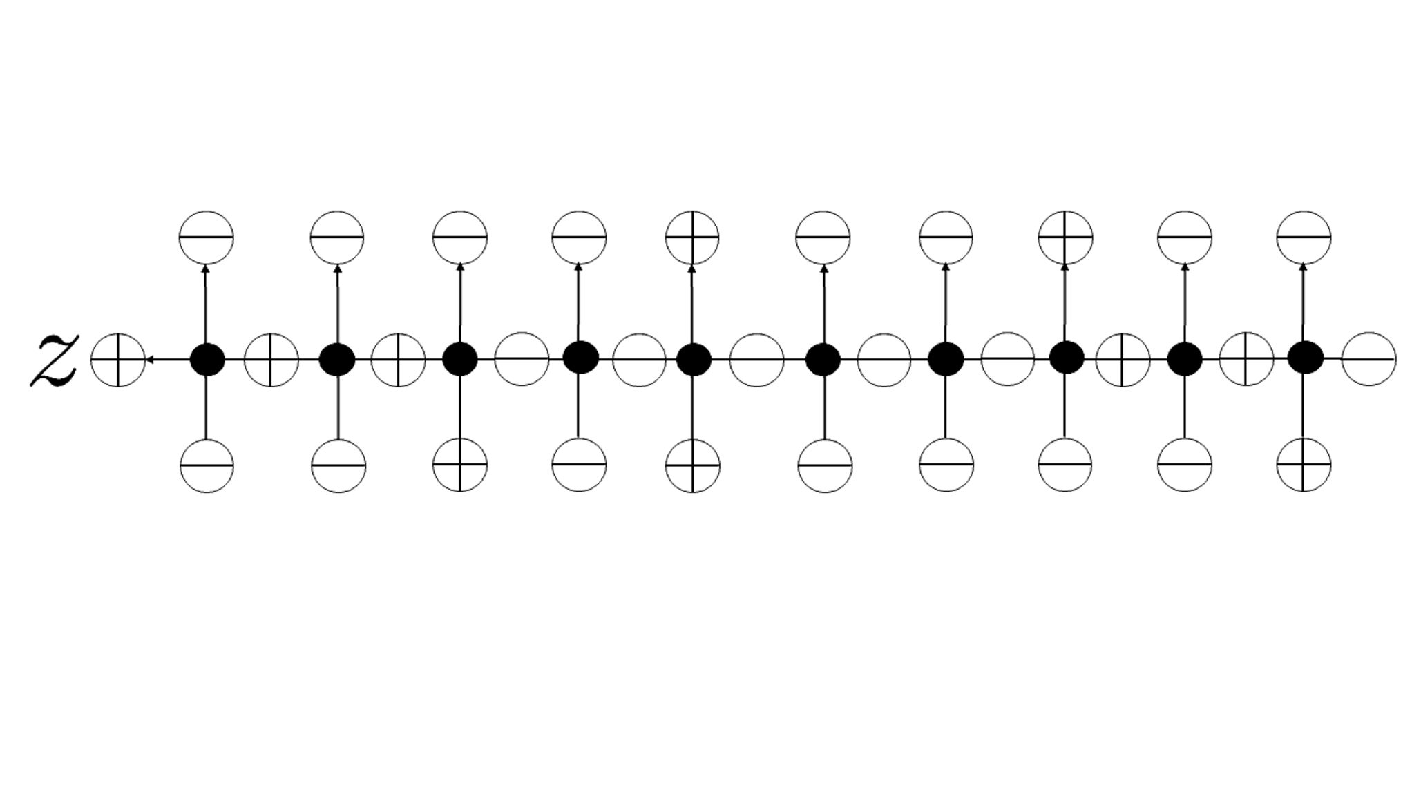
Example (coordinate representation) Let M=10M=10, N=2N=2, x¯=(3,6)\overline{x}=(3,6) and y¯=(1,6,8)\overline{y}=(1,6,8). We also set x3¯=10+1=11\overline{x_{3}}=10+1=11. From Max⁡(x1¯−y1¯−1,0)=Max⁡(3−1−1,0)=1\mathrm{Max}(\overline{x_{1}}-\overline{y_{1}}-1,0)=\mathrm{Max}(3-1-1,0)=1, Max⁡(x2¯−y2¯−1,0)=Max⁡(6−6−1,0)=0\mathrm{Max}(\overline{x_{2}}-\overline{y_{2}}-1,0)=\mathrm{Max}(6-6-1,0)=0, Max⁡(x3¯−y3¯−1,0)=Max⁡(11−8−1,0)=2\mathrm{Max}(\overline{x_{3}}-\overline{y_{3}}-1,0)=\mathrm{Max}(11-8-1,0)=2, we have the factor t2+0+1=t3t^{2+0+1}=t^{3}. The relations y1¯≠x1¯≠y2¯\overline{y_{1}}\neq\overline{x_{1}}\neq\overline{y_{2}}, y2¯=x2¯≠y3¯\overline{y_{2}}=\overline{x_{2}}\neq\overline{y_{3}} give the factor (t+1)1=t+1(t+1)^{1}=t+1, and we also have the factor z5z^{5} from (y2¯−x1¯)+(y3¯−x2¯)=(6−3)+(8−6)=3+2=5(\overline{y_{2}}-\overline{x_{1}})+(\overline{y_{3}}-\overline{x_{2}})=(6-3)+(8-6)=3+2=5. In total, the right hand side of (6.1) is calculated as (t+1)​t3​z5(t+1)t^{3}z^{5}. One can check that this matches the left hand side of (6.1), i.e., the matrix elements of the corresponding BB-operator by explicit calculation (see Figure 7 for a graphical description of the corresponding matrix element).

Example (Young diagram representation) Let M=10M=10, N=2N=2, x¯=(3,6)\overline{x}=(3,6) and y¯=(1,6,8)\overline{y}=(1,6,8). We have λ¯=(6−2,3−1)=(4,2)\overline{\lambda}=(6-2,3-1)=(4,2) and μ¯=(8−3,6−2,1−1)=(5,4,0)\overline{\mu}=(8-3,6-2,1-1)=(5,4,0). We also set λ0¯=10−2=8\overline{\lambda_{0}}=10-2=8. From Max⁡(λ0¯−μ1¯−1,0)=Max⁡(8−5−1,0)=2\mathrm{Max}(\overline{\lambda_{0}}-\overline{\mu_{1}}-1,0)=\mathrm{Max}(8-5-1,0)=2, Max⁡(λ1¯−μ2¯−1,0)=Max⁡(4−4−1,0)=0\mathrm{Max}(\overline{\lambda_{1}}-\overline{\mu_{2}}-1,0)=\mathrm{Max}(4-4-1,0)=0, Max⁡(λ2¯−μ3¯−1,0)=Max⁡(2−0−1,0)=1\mathrm{Max}(\overline{\lambda_{2}}-\overline{\mu_{3}}-1,0)=\mathrm{Max}(2-0-1,0)=1, we have the factor t2+0+1=t3t^{2+0+1}=t^{3}. The relations μ1¯+1≠λ1¯=μ2¯\overline{\mu_{1}}+1\neq\overline{\lambda_{1}}=\overline{\mu_{2}}, μ2¯+1≠λ2¯≠μ3¯\overline{\mu_{2}}+1\neq\overline{\lambda_{2}}\neq\overline{\mu_{3}} give the factor (t+1)1=t+1(t+1)^{1}=t+1, and we also have the factor z5z^{5} from (μ1¯−λ1¯)+(μ2¯−λ2¯)+2=(5−4)+(4−2)+2=5(\overline{\mu_{1}}-\overline{\lambda_{1}})+(\overline{\mu_{2}}-\overline{\lambda_{2}})+2=(5-4)+(4-2)+2=5. Altogether, the right hand side of (6.2) is calculated as (t+1)​t3​z5(t+1)t^{3}z^{5}.

Refer to caption
Figure 7: The matrix element ⟨x1¯⋯xN¯|B(z)|y1¯⋯yN+1¯⟩\langle\overline{x_{1}}\cdots\overline{x_{N}}|B(z)|\overline{y_{1}}\cdots\overline{y_{N+1}}\rangle for M=10M=10, N=2N=2, x¯=(3,6)\overline{x}=(3,6) and y¯=(1,6,8)\overline{y}=(1,6,8). One sees that the inner state is uniquely fixed, and the matrix element is calculated by multiplying the matrix elements of the LL-operators t×t×1×z×z×z×z×(t+1)​z×t×1=(t+1)​t3​z5t\times t\times 1\times z\times z\times z\times z\times(t+1)z\times t\times 1=(t+1)t^{3}z^{5}.

In order to descibe the microscopic structure, we introduce the following strict dual Gelfand-Tsetlin patterns

𝒯¯={aN−1,N−1¯⋰⋱a1,1¯⋯a1,N−1¯a0,0¯a0,1¯⋯a0,N−2¯a0,N−1¯},\displaystyle\overline{\mathcal{T}}=\left\{\begin{array}[]{ccccccc}&&&\overline{a_{N-1,N-1}}&&&\\ &&\iddots&&\ddots&&\\ &\overline{a_{1,1}}&&\cdots&&\overline{a_{1,N-1}}&\\ \overline{a_{0,0}}&&\overline{a_{0,1}}&\cdots&\overline{a_{0,N-2}}&&\overline{a_{0,N-1}}\end{array}\right\},

in which the rows interlace ai−1,j−1¯≥ai,j¯≥ai−1,j¯\overline{a_{i-1,j-1}}\geq\overline{a_{i,j}}\geq\overline{a_{i-1,j}}, and the entries in horizontal rows are strictly decreasing. We use this picture so as to be consistent with the dual wavefunction description. The strict Gelfand-Tsetlin patterns essentially label the inner states by recording the positions of the holes in the auxiliary spaces.

For each strict Gelfand-Tsetlin pattern, we assign the following weight:

G¯(𝒯¯,{z}N)=∏i=0N−1∏j=iN−1γ¯(ai,j¯)zNd0​(𝒯¯)−d1​(𝒯¯)zN−1d1​(𝒯¯)−d2​(𝒯¯)⋯z2dN−2​(𝒯¯)−dN−1​(𝒯¯)z1dN−1​(𝒯¯),\displaystyle\overline{G}(\overline{\mathcal{T}},\{z\}_{N})=\prod_{i=0}^{N-1}\prod_{j=i}^{N-1}\overline{\gamma}(\overline{a_{i,j}})z_{N}^{d_{0}(\overline{\mathcal{T}})-d_{1}(\overline{\mathcal{T}})}z_{N-1}^{d_{1}(\overline{\mathcal{T}})-d_{2}(\overline{\mathcal{T}})}\cdots z_{2}^{d_{N-2}(\overline{\mathcal{T}})-d_{N-1}(\overline{\mathcal{T}})}z_{1}^{d_{N-1}(\overline{\mathcal{T}})}, (6.8)

where dj​(𝒯¯)=∑k=jN−1aj,k¯d_{j}(\overline{\mathcal{T}})=\sum_{k=j}^{N-1}\overline{a_{j,k}}, j=0,…,N−1j=0,\dots,N-1 is the sum of the entries of the Gelfand-Tsetlin pattern in the jj-th row counted from the bottom, and γ¯​(ai,j¯)\overline{\gamma}(\overline{a_{i,j}}) is defined as

γ¯​(ai,j¯)=tMax⁡(ai+1,j¯−ai,j¯−1,0)×{t+1ai−1,j¯≠ai,j¯≠ai−1,j−1¯1otherwise,\displaystyle\overline{\gamma}(\overline{a_{i,j}})=t^{\mathrm{Max}(\overline{a_{i+1,j}}-\overline{a_{i,j}}-1,0)}\times\left\{\begin{array}[]{ll}t+1&\overline{a_{i-1,j}}\neq\overline{a_{i,j}}\neq\overline{a_{i-1,j-1}}\\ 1&\mathrm{otherwise}\end{array}\right.,

for pairs of integers (i,j)(i,j) satisfying 0≤i≤N−1,i≤j≤N−10\leq i\leq N-1,\ i\leq j\leq{N-1}. Note that we define γ¯​(a0,j¯)\overline{\gamma}(\overline{a_{0,j}}), j=0,…,N−1j=0,\dots,N-1 since we need these weights to describe the dual wavefunction and the dual Tokuyama-type formula (whereas one does not need to define γ⁡(a0,j)\gamma(a_{0,j}) to describe the original wavefunction and the Tokuyama formula). We also define aj,j−1¯=M\overline{a_{j,j-1}}=M for j=1,⋯,Nj=1,\cdots,N.

As again, the inner states making non-zero contributions can be characterized by the strict Gelfand-Tsetlin pattern with the bottom row fixed by the Young diagram as a0,j¯=λj+1¯+N−j−1\overline{a_{0,j}}=\overline{\lambda_{j+1}}+N-j-1.

Theorem 6.2.

We have the following combinatorial formula for the Schur polynomials

tN⁡(M−N)​∏1≤j<k≤N(zj+t​zk)​sλ¯​({zt}N)\displaystyle t^{N(M-N)}\prod_{1\leq j<k\leq N}(z_{j}+tz_{k})s_{\overline{\lambda}}\Bigg(\Bigg\{\frac{z}{t}\Bigg\}_{N}\Bigg)
=\displaystyle= ∑𝒯¯G¯​(𝒯¯,{z}N)\displaystyle\sum_{\overline{\mathcal{T}}}\overline{G}(\overline{\mathcal{T}},\{z\}_{N})
=\displaystyle= ∑𝒯¯∏i=0N−1∏j=iN−1γ¯(ai,j¯)zNd0​(𝒯¯)−d1​(𝒯¯)zN−1d1​(𝒯¯)−d2​(𝒯¯)⋯z2dN−2​(𝒯¯)−dN−1​(𝒯¯)z1dN−1​(𝒯¯),\displaystyle\sum_{\overline{\mathcal{T}}}\prod_{i=0}^{N-1}\prod_{j=i}^{N-1}\overline{\gamma}(\overline{a_{i,j}})z_{N}^{d_{0}(\overline{\mathcal{T}})-d_{1}(\overline{\mathcal{T}})}z_{N-1}^{d_{1}(\overline{\mathcal{T}})-d_{2}(\overline{\mathcal{T}})}\cdots z_{2}^{d_{N-2}(\overline{\mathcal{T}})-d_{N-1}(\overline{\mathcal{T}})}z_{1}^{d_{N-1}(\overline{\mathcal{T}})}, (6.11)

where the sum is over all strict Gelfand-Tsetlin patterns with the bottom row of the strict Gelfand-Tsetlin pattern is fixed by the Young diagram as a0,j¯=λj+1¯+N−j−1\overline{a_{0,j}}=\overline{\lambda_{j+1}}+N-j-1.

Proof.

The proof follows from evaluating the dual wavefunction
⟨Φ(z1,…,zN)|x1¯⋯xN¯⟩=⟨1⋯M|B(z1)⋯B(zN)|x1¯⋯xN¯⟩\langle\Phi(z_{1},\dots,z_{N})|\overline{x_{1}}\cdots\overline{x_{N}}\rangle=\langle 1\cdots M|B(z_{1})\cdots B(z_{N})|\overline{x_{1}}\cdots\overline{x_{N}}\rangle in two ways. First, we note from Theorem 4.1 that ⟨1⋯M|B(z1)⋯B(zN)|x1¯⋯xN¯⟩\langle 1\cdots M|B(z_{1})\cdots B(z_{N})|\overline{x_{1}}\cdots\overline{x_{N}}\rangle is expressed using Schur polynomials as (4.3).

Another way of evaluation can be accomplished by viewing the dual wavefunction as a partition function constructed from NN layers of BB-operators, inserting the completeness relation and decomposing it as sums of products of matrix elements of the BB-operators. That is, we decompose the dual wavefunction as

⟨1⋯M|B(z1)⋯B(zN)|x1¯⋯xN¯⟩\displaystyle\langle 1\cdots M|B(z_{1})\cdots B(z_{N})|\overline{x_{1}}\cdots\overline{x_{N}}\rangle
=\displaystyle= ∑𝒯¯⟨1⋯M|\displaystyle\sum_{\overline{\mathcal{T}}}\langle 1\cdots M|
×∏j=1N{|aN−j+1,N−1¯+1,⋯,aN−j+1,N−j+1¯+1⟩⟨aN−j+1,N−1¯+1,⋯,aN−j+1,N−j+1¯+1|B(zj)}\displaystyle\times\prod_{j=1}^{N}\Bigg\{|\overline{a_{N-j+1,N-1}}+1,\cdots,\overline{a_{N-j+1,N-j+1}}+1\rangle\langle\overline{a_{N-j+1,N-1}}+1,\cdots,\overline{a_{N-j+1,N-j+1}}+1|B(z_{j})\Bigg\}
×|a0,N−1¯+1⋯a0,0¯+1⟩,\displaystyle\times|\overline{a_{0,N-1}}+1\cdots\overline{a_{0,0}}+1\rangle, (6.12)

where

|aj,N−1¯+1⋯aj,j¯+1⟩=∏k=jN−1σaj,k¯+1+(|1⟩1⊗⋯⊗|1⟩M),\displaystyle|\overline{a_{j,N-1}}+1\cdots\overline{a_{j,j}}+1\rangle=\prod_{k=j}^{N-1}\sigma_{\overline{a_{j,k}}+1}^{+}(|1\rangle_{1}\otimes\cdots\otimes|1\rangle_{M}), (6.13)
⟨aj,N−1¯+1⋯aj,j¯+1|=(⟨1|1⊗⋯⊗⟨1|M)∏k=jN−1σaj,k¯+1−.\displaystyle\langle\overline{a_{j,N-1}}+1\cdots\overline{a_{j,j}}+1|=(\langle 1|_{1}\otimes\cdots\otimes\langle 1|_{M})\prod_{k=j}^{N-1}\sigma_{\overline{a_{j,k}}+1}^{-}. (6.14)

and use the formula for the matrix elements of a single BB-operator (6.1) in Proposition 6.1. Then one finds the product of the matrix elements of the BB-operators in (6.12) corresponding to each strict Gelfand-Tsetlin pattern 𝒯¯\overline{\mathcal{T}} can be expressed as (6.8)

G¯(𝒯¯,{z}N)=∏i=0N−1∏j=iN−1γ¯(ai,j¯)zNd0​(𝒯¯)−d1​(𝒯¯)zN−1d1​(𝒯¯)−d2​(𝒯¯)⋯z2dN−2​(𝒯¯)−dN−1​(𝒯¯)z1dN−1​(𝒯¯).\displaystyle\overline{G}(\overline{\mathcal{T}},\{z\}_{N})=\prod_{i=0}^{N-1}\prod_{j=i}^{N-1}\overline{\gamma}(\overline{a_{i,j}})z_{N}^{d_{0}(\overline{\mathcal{T}})-d_{1}(\overline{\mathcal{T}})}z_{N-1}^{d_{1}(\overline{\mathcal{T}})-d_{2}(\overline{\mathcal{T}})}\cdots z_{2}^{d_{N-2}(\overline{\mathcal{T}})-d_{N-1}(\overline{\mathcal{T}})}z_{1}^{d_{N-1}(\overline{\mathcal{T}})}. (6.15)

Hence, the identity (6.12) can be rewritten in the following form for the dual wavefunction

⟨1⋯M|B(z1)⋯B(zN)|x1¯⋯xN¯⟩\displaystyle\langle 1\cdots M|B(z_{1})\cdots B(z_{N})|\overline{x_{1}}\cdots\overline{x_{N}}\rangle
=\displaystyle= ∑𝒯¯G¯​(𝒯¯,{z}N)\displaystyle\sum_{\overline{\mathcal{T}}}\overline{G}(\overline{\mathcal{T}},\{z\}_{N})
=\displaystyle= ∑𝒯¯∏i=0N−1∏j=iN−1γ¯(ai,j¯)zNd0​(𝒯¯)−d1​(𝒯¯)zN−1d1​(𝒯¯)−d2​(𝒯¯)⋯z2dN−2​(𝒯¯)−dN−1​(𝒯¯)z1dN−1​(𝒯¯).\displaystyle\sum_{\overline{\mathcal{T}}}\prod_{i=0}^{N-1}\prod_{j=i}^{N-1}\overline{\gamma}(\overline{a_{i,j}})z_{N}^{d_{0}(\overline{\mathcal{T}})-d_{1}(\overline{\mathcal{T}})}z_{N-1}^{d_{1}(\overline{\mathcal{T}})-d_{2}(\overline{\mathcal{T}})}\cdots z_{2}^{d_{N-2}(\overline{\mathcal{T}})-d_{N-1}(\overline{\mathcal{T}})}z_{1}^{d_{N-1}(\overline{\mathcal{T}})}. (6.16)

Comparing the two expressions (4.3) and (6.16) evaluated by two ways, we get (6.11).

∎

The combinatorial formula (6.11) in Theorem 6.2 can be rewritten into the following form by scaling every spectral parameter zjz_{j} to t​zjtz_{j} and cancelling powers of tt of both hand sides and simplyfing.

Theorem 6.3.

We have the following combinatorial formula for the Schur polynomials

∏1≤j<k≤N(zj+t​zk)​sλ¯​({z}N)\displaystyle\prod_{1\leq j<k\leq N}(z_{j}+tz_{k})s_{\overline{\lambda}}(\{z\}_{N})
=\displaystyle= t∑j=1Nλj¯−N⁡(M−N)∑𝒯¯∏i=0N−1∏j=iN−1γ¯(ai,j¯)zNd0​(𝒯¯)−d1​(𝒯¯)zN−1d1​(𝒯¯)−d2​(𝒯¯)⋯z2dN−2​(𝒯¯)−dN−1​(𝒯¯)z1dN−1​(𝒯¯),\displaystyle t^{\sum_{j=1}^{N}\overline{\lambda_{j}}-N(M-N)}\sum_{\overline{\mathcal{T}}}\prod_{i=0}^{N-1}\prod_{j=i}^{N-1}\overline{\gamma}(\overline{a_{i,j}})z_{N}^{d_{0}(\overline{\mathcal{T}})-d_{1}(\overline{\mathcal{T}})}z_{N-1}^{d_{1}(\overline{\mathcal{T}})-d_{2}(\overline{\mathcal{T}})}\cdots z_{2}^{d_{N-2}(\overline{\mathcal{T}})-d_{N-1}(\overline{\mathcal{T}})}z_{1}^{d_{N-1}(\overline{\mathcal{T}})}, (6.17)

where the sum is over all strict Gelfand-Tsetlin patterns with the bottom row of the strict Gelfand-Tsetlin pattern is fixed by the Young diagram as a0,j¯=λj+1¯+N−j−1\overline{a_{0,j}}=\overline{\lambda_{j+1}}+N-j-1.

Let us discuss the differences between Theorem 3.3 and Theorem 6.3. In the original wavefunction, the factor γ⁡(ai,j)\gamma(a_{i,j}) (3) in (3.16) depends only on three neighbors ai,ja_{i,j}, ai−1,ja_{i-1,j} and ai−1,j−1a_{i-1,j-1} in the strict Gelfand-Tsetlin pattern. On the other hand, for the case of the dual wavefunction, the factor γ¯​(ai,j¯)\overline{\gamma}(\overline{a_{i,j}}) (6) in (6.17) depends on four neighbors ai,j¯\overline{a_{i,j}}, ai−1,j¯\overline{a_{i-1,j}}, ai−1,j−1¯\overline{a_{i-1,j-1}} and ai+1,j¯\overline{a_{i+1,j}}. Note also the order of the symmetric variables (spectral parameters) in (3.16) is z1,…,zNz_{1},\dots,z_{N}, while it is zN,…,z1z_{N},\dots,z_{1} in (6.17), i.e., the order is reversed. Moreover, the right hand side of (6.17) has powers of tt as factors, which explicitly depends on the size of the Young diagram, the total number of sites MM and the total number of holes NN. This explicit dependence cannot be found in (3.16).

Example Let us check (6.17) by an example. Consider the case M=4M=4, N=2N=2, λ¯=(λ¯1,λ2¯)=(2,1)\overline{\lambda}=(\overline{\lambda}_{1},\overline{\lambda_{2}})=(2,1). The bottom row of the dual strict Gelfand-Tsetlin pattern is fixed as a0,0¯=λ1¯+N−0−1=2+2−0−1=3\overline{a_{0,0}}=\overline{\lambda_{1}}+N-0-1=2+2-0-1=3, a0,1¯=λ2¯+N−1−1=1+2−1−1=1\overline{a_{0,1}}=\overline{\lambda_{2}}+N-1-1=1+2-1-1=1. From the interlacing relation 3=a0,0¯≥a1,1¯≥a0,1¯=13=\overline{a_{0,0}}\geq\overline{a_{1,1}}\geq\overline{a_{0,1}}=1, we have a1,1¯=1\overline{a_{1,1}}=1, 22 or 33. Therefore, there are three strict Gelfand-Tsetlin patterns in the sum of (6.17)

𝒯¯={a1,1¯a0,0¯a0,1¯}\displaystyle\overline{\mathcal{T}}=\left\{\begin{array}[]{ccc}&\overline{a_{1,1}}&\\ \overline{a_{0,0}}&&\overline{a_{0,1}}\end{array}\right\}
=\displaystyle= {131},{231},{331}.\displaystyle\left\{\begin{array}[]{ccc}&1&\\ 3&&1\end{array}\right\},\ \left\{\begin{array}[]{ccc}&2&\\ 3&&1\end{array}\right\},\ \left\{\begin{array}[]{ccc}&3&\\ 3&&1\end{array}\right\}.

We also set a1,0¯=a2,1¯=4\overline{a_{1,0}}=\overline{a_{2,1}}=4 for each strict Gelfand-Tsetlin pattern. Keeping this in mind, let us calculate the weights for each pattern.

(1) 𝒯¯={131}.\displaystyle\overline{\mathcal{T}}=\left\{\begin{array}[]{ccc}&1&\\ 3&&1\end{array}\right\}.
We have γ¯​(a0,0¯)=tMax⁡(4−3−1,0)=1\overline{\gamma}(\overline{a_{0,0}})=t^{\mathrm{Max}(4-3-1,0)}=1, γ¯​(a0,1¯)=tMax⁡(1−1−1,0)=1\overline{\gamma}(\overline{a_{0,1}})=t^{\mathrm{Max}(1-1-1,0)}=1, γ¯​(a1,1¯)=tMax⁡(4−1−1,0)=t2\overline{\gamma}(\overline{a_{1,1}})=t^{\mathrm{Max}(4-1-1,0)}=t^{2}, d0​(𝒯¯)=3+1=4d_{0}(\overline{\mathcal{T}})=3+1=4, d1​(𝒯¯)=1d_{1}(\overline{\mathcal{T}})=1. Thus we have γ¯​(a0,0¯)​γ¯​(a0,1¯)​γ¯​(a1,1¯)​z2d0​(𝒯¯)−d1​(𝒯¯)​z1d1​(𝒯¯)=t2​z23​z1\overline{\gamma}(\overline{a_{0,0}})\overline{\gamma}(\overline{a_{0,1}})\overline{\gamma}(\overline{a_{1,1}})z_{2}^{d_{0}(\overline{\mathcal{T}})-d_{1}(\overline{\mathcal{T}})}z_{1}^{d_{1}(\overline{\mathcal{T}})}=t^{2}z_{2}^{3}z_{1}.

(2) 𝒯¯={231}.\displaystyle\overline{\mathcal{T}}=\left\{\begin{array}[]{ccc}&2&\\ 3&&1\end{array}\right\}.
We have γ¯​(a0,0¯)=tMax⁡(4−3−1,0)=1\overline{\gamma}(\overline{a_{0,0}})=t^{\mathrm{Max}(4-3-1,0)}=1, γ¯​(a0,1¯)=tMax⁡(2−1−1,0)=1\overline{\gamma}(\overline{a_{0,1}})=t^{\mathrm{Max}(2-1-1,0)}=1, γ¯​(a1,1¯)=tMax⁡(4−2−1,0)​(t+1)=t⁡(t+1)\overline{\gamma}(\overline{a_{1,1}})=t^{\mathrm{Max}(4-2-1,0)}(t+1)=t(t+1), d0​(𝒯¯)=3+1=4d_{0}(\overline{\mathcal{T}})=3+1=4, d1​(𝒯¯)=2d_{1}(\overline{\mathcal{T}})=2. The corresponding weight is
γ¯​(a0,0¯)​γ¯​(a0,1¯)​γ¯​(a1,1¯)​z2d0​(𝒯¯)−d1​(𝒯¯)​z1d1​(𝒯¯)=t⁡(t+1)​z22​z12\overline{\gamma}(\overline{a_{0,0}})\overline{\gamma}(\overline{a_{0,1}})\overline{\gamma}(\overline{a_{1,1}})z_{2}^{d_{0}(\overline{\mathcal{T}})-d_{1}(\overline{\mathcal{T}})}z_{1}^{d_{1}(\overline{\mathcal{T}})}=t(t+1)z_{2}^{2}z_{1}^{2}.

(3) 𝒯¯={331}.\displaystyle\overline{\mathcal{T}}=\left\{\begin{array}[]{ccc}&3&\\ 3&&1\end{array}\right\}.
We have γ¯​(a0,0¯)=tMax⁡(4−3−1,0)=1\overline{\gamma}(\overline{a_{0,0}})=t^{\mathrm{Max}(4-3-1,0)}=1, γ¯​(a0,1¯)=tMax⁡(3−1−1,0)=t\overline{\gamma}(\overline{a_{0,1}})=t^{\mathrm{Max}(3-1-1,0)}=t, γ¯​(a1,1¯)=tMax⁡(4−3−1,0)=1\overline{\gamma}(\overline{a_{1,1}})=t^{\mathrm{Max}(4-3-1,0)}=1, d0​(𝒯¯)=3+1=4d_{0}(\overline{\mathcal{T}})=3+1=4, d1​(𝒯¯)=3d_{1}(\overline{\mathcal{T}})=3. We have γ¯​(a0,0¯)​γ¯​(a0,1¯)​γ¯​(a1,1¯)​z2d0​(𝒯¯)−d1​(𝒯¯)​z1d1​(𝒯¯)=t​z2​z13\overline{\gamma}(\overline{a_{0,0}})\overline{\gamma}(\overline{a_{0,1}})\overline{\gamma}(\overline{a_{1,1}})z_{2}^{d_{0}(\overline{\mathcal{T}})-d_{1}(\overline{\mathcal{T}})}z_{1}^{d_{1}(\overline{\mathcal{T}})}=tz_{2}z_{1}^{3} in total.

Summing the three weights calculated above and noting ∑j=12λj¯−N⁡(M−N)=2+1−4=−1\sum_{j=1}^{2}\overline{\lambda_{j}}-N(M-N)=2+1-4=-1, the right hand side of (6.17) is t−1​(t2​z23​z1+t⁡(t+1)​z22​z12+t​z2​z13)=t​z23​z1+(t+1)​z22​z12+z2​z13t^{-1}(t^{2}z_{2}^{3}z_{1}+t(t+1)z_{2}^{2}z_{1}^{2}+tz_{2}z_{1}^{3})=tz_{2}^{3}z_{1}+(t+1)z_{2}^{2}z_{1}^{2}+z_{2}z_{1}^{3}, which can be factorized as (z1+t​z2)​(z12​z2+z1​z22)=(z1+t​z2)​s(2,1)​(z1,z2)(z_{1}+tz_{2})(z_{1}^{2}z_{2}+z_{1}z_{2}^{2})=(z_{1}+tz_{2})s_{(2,1)}(z_{1},z_{2}), which is exactly the left hand side of (6.17).

7 A generalization of the correspondence

We have showed Theorem 4.1 which gives the relation between the dual wavefunction and the Schur polynomials, for which we gave two proofs. The one given in section 4 can be applied to a generalization of the Felderhof model, where inhomogeneous parameters are now introduced in the quantum spaces. Since the original wavefunction was found to give the factorial Schur polynomials [16], one expects the dual wavefunction also gives the factorial Schur polynomials.

The LL-operator which constructs the wavefunction now has dependence on the quantum space ℱj\mathcal{F}_{j}: at the jj-th site in the quantum space, we introduce the following LL-operator

La​j​(z,t,αj)=(10000t100(t+1)​zz+αj0000z−t​αj).\displaystyle L_{aj}(z,t,\alpha_{j})=\left(\begin{array}[]{cccc}1&0&0&0\\ 0&t&1&0\\ 0&(t+1)z&z+\alpha_{j}&0\\ 0&0&0&z-t\alpha_{j}\end{array}\right).

The LL-operators La​j​(z,t,αj)L_{aj}(z,t,\alpha_{j}) now has inhomogeneous parameters αj\alpha_{j}, j=1,⋯Mj=1,\cdots M besides the spectral parameter and the deformation parameters.

We consider the wavefunction ⟨x1⋯xN|Ψ(z1,…,zN,{α})⟩\langle x_{1}\cdots x_{N}|\Psi(z_{1},\dots,z_{N},\{\alpha\})\rangle by introducing the NN-particle state

Ψ(z1,…,zN,{α})⟩=B(z1,{α})⋯B(zN,{α})|Ω⟩,\displaystyle\Psi(z_{1},\dots,z_{N},\{\alpha\})\rangle=B(z_{1},\{\alpha\})\cdots B(z_{N},\{\alpha\})|\Omega\rangle, (7.6)

where the BB-operator

B(z,{α})=⟨0|La​M(z,t,αM)⋯La​1(z,t,α1)|1⟩aa,\displaystyle B(z,\{\alpha\})={}_{a}\langle 0|L_{aM}(z,t,\alpha_{M})\cdots L_{a1}(z,t,\alpha_{1})|1\rangle_{a}, (7.7)

now has dependence on the inhomogeneous parameters {α}={α1,…,αM}\{\alpha\}=\{\alpha_{1},\dots,\alpha_{M}\}, which turns out to be the factorial parameters of the factorial Schur polynomials defined below.

Definition 7.1.

The factorial Schur polynomials is defined to be the following determinant:

sλ​({z}N​|{α}|)=Fλ+δ​({z}N|{α})∏1≤j<k≤N(zj−zk),\displaystyle s_{\lambda}(\{z\}_{N}|\{\alpha\}|)=\frac{F_{\lambda+\delta}(\{z\}_{N}|\{\alpha\})}{\prod_{1\leq j<k\leq N}(z_{j}-z_{k})}, (7.8)

where {z}={z1,…,zN}\{z\}=\{z_{1},\dots,z_{N}\} is a set of variables and λ\lambda denotes a Young diagram λ=(λ1,λ2,…,λN)\lambda=(\lambda_{1},\lambda_{2},\dots,\lambda_{N}) with weakly decreasing non-negative integers λ1≥λ2≥⋯≥λN≥0\lambda_{1}\geq\lambda_{2}\geq\cdots\geq\lambda_{N}\geq 0, and δ=(N−1,N−2,…,0)\delta=(N-1,N-2,\dots,0). Fμ​({z}N|{α})F_{\mu}(\{z\}_{N}|\{\alpha\}) is an N×NN\times N determinant

Fμ​({z}N|{α})=detN​(∏j=1μ(zk+αj)).\displaystyle F_{\mu}(\{z\}_{N}|\{\alpha\})=\mathrm{det}_{N}\Bigg(\prod_{j=1}^{\mu}(z_{k}+\alpha_{j})\Bigg). (7.9)

We remark that one must respect the ordering of the factorial parameters {α}={α1,…,αM}\{\alpha\}=\{\alpha_{1},\dots,\alpha_{M}\}.

Bump, McNamara and Nakasuji showed the following correspondence between the wavefunction of the Felderhof model with inhomogeneties and the factorial Schur polynomials.

Theorem 7.2.

[16] The wavefunction ⟨x1​…​xN|Ψ⁡(z1,…,zN,{α})⟩\langle x_{1}\dots x_{N}|\Psi(z_{1},\dots,z_{N},\{\alpha\})\rangle is expressed by the factorial Schur polynomials as

⟨x1​…​xN|Ψ⁡(z1,…,zN,{α})⟩=∏1≤j<k≤N(zj+t​zk)​sλ​({z}N|{α}),\displaystyle\langle x_{1}\dots x_{N}|\Psi(z_{1},\dots,z_{N},\{\alpha\})\rangle=\prod_{1\leq j<k\leq N}(z_{j}+tz_{k})s_{\lambda}(\{z\}_{N}|\{\alpha\}), (7.10)

under the relation λj=xN−j+1−N+j−1\lambda_{j}=x_{N-j+1}-N+j-1, j=1,…,Nj=1,\dots,N.

This Theorem was proved by noting that the arguments in [13] naturally lift to this inhomogeneous setting. One first shows that the wavefunction is a polynomial of tt with highest weight degree N⁡(N−1)/2N(N-1)/2. Then one evaluates the wavefunction at t=−1t=-1, at which the six-vertex model reduces to a five-vertex model, and each configuration making nonzero contribution to the wavefunction essentially corrresponds to each term of the determinant expansion of the numerator of the factorial Schur polynomials (7.8).

Let us now state the result for the dual wavefunction ⟨Φ(z1,…,zN,{α})|x1¯⋯xN¯⟩\langle\Phi(z_{1},\dots,z_{N},\{\alpha\})|\overline{x_{1}}\cdots\overline{x_{N}}\rangle which is the overlap between the hole configurations |x1¯⋯xN¯⟩|\overline{x_{1}}\cdots\overline{x_{N}}\rangle and the dual NN-particle state

⟨Φ(z1,…,zN,{α})|=⟨1⋯M|B(z1,{α})⋯B(zN,{α}).\displaystyle\langle\Phi(z_{1},\dots,z_{N},\{\alpha\})|=\langle 1\cdots M|B(z_{1},\{\alpha\})\cdots B(z_{N},\{\alpha\}). (7.11)

By applying the argument in section 4, one gets the following relation between the dual wavefunction and the factorial Schur polynomials.

Theorem 7.3.

The dual wavefunction ⟨Φ(z1,…,zN,{α})|x1¯⋯xN¯⟩\langle\Phi(z_{1},\dots,z_{N},\{\alpha\})|\overline{x_{1}}\cdots\overline{x_{N}}\rangle can be expressed by the factorial Schur polynomials as

⟨Φ(z1,…,zN,{α})|x1¯⋯xN¯⟩=tN⁡(M−N)∏1≤j<k≤N(zj+tzk)sλ¯({zt}N,{−α}).\displaystyle\langle\Phi(z_{1},\dots,z_{N},\{\alpha\})|\overline{x_{1}}\cdots\overline{x_{N}}\rangle=t^{N(M-N)}\prod_{1\leq j<k\leq N}(z_{j}+tz_{k})s_{\overline{\lambda}}\Bigg(\Bigg\{\frac{z}{t}\Bigg\}_{N},\{-\alpha\}\Bigg). (7.12)

Here the Young diagram for the factorial Schur polynomials correspond to the particle configuration under the relation λj¯=xN−j+1¯−N+j−1\overline{\lambda_{j}}=\overline{x_{N-j+1}}-N+j-1, j=1,…,Nj=1,\dots,N, and the symmetric variables are {zt}N={z1t,…,zNt}\displaystyle\Bigg\{\frac{z}{t}\Bigg\}_{N}=\Bigg\{\frac{z_{1}}{t},\dots,\frac{z_{N}}{t}\Bigg\}. Moreover, the signs of the parameters of the factorial Schur polynomials in the right hand side of (7.12) are now inverted simultaneously: {−α}={−α1,…,−αM}\{-\alpha\}=\{-\alpha_{1},\dots,-\alpha_{M}\}.

The correspondence (7.12) includes the special case t=1t=1 of the relation between the dual wavefunction and factorial Schur polynomials in [16], which was proved by starting from the result for the relation between the original wavefunction and the factorial Schur polynomials, using arguments on the symmetry of the LL-operators to transform the original correspondence to the dual correspondence. This argument seems very difficult for the case t≠1t\neq 1 even for the ordinary Schur polynomials. However, one can naturally lift the arguments given in section 4 to this inhomogeneous setting. The problem reduces to the case of the t=−1t=-1, where the six-vertex model reduces to the five-vertex model. Since we now have the inhomogenous parameters, this introduction of additional parameters is reflected in the final expression of the correspondence in (7.12).

8 Conclusion

We investigated the Felderhof free-fermion model, and analyzed the dual wavefunction in two ways. We first showed the precise relation between the dual wavefunction and the Schur polynomials, in which we gave two proofs in sections 4 and 5 respectively. One by using the arguments by [13], and another one by combining the matrix product method and the analysis on the domain wall boundary partition function. Next, by calculating the matrix elements of a single BB-operator, we give a combinatorial expression of the Schur polynomials in terms of strict Gelfand-Tsetlin patterns. By comparing the two expressions, we obtained a combinatorial formula of the Schur polynomials, which can be regarded as a dual version of the Tokuyama formula, since it was found [13] that the original wavefunction naturally gives a realization of the Tokuyama formula for the Schur polynomials, and we are now dealing with the dual wavefunction.

We also generalized the relation between the dual wavefunction to the Felderhof model with inhomogeneous parameters in the quantum space and the factorial Schur polynomials, which is motivated by the fact that the wavefunction of the Felderhof model with inhomogeneties are given by the factorial Schur polynomials [16]. The expression can be extended furthermore to the Felderhof model with two types of inhomogeneous parameters, and there are correspondences between the original and the dual wavefunctions and a generalization of the factorial Schur polynomials [22, 23].

One of the important problems related to this paper is to study the dual wavefunction for the case of other boundary conditions and find combinatorial formulas for other symmetric polynomials such as the symplectic Schur and Schur QQ functions. See [24, 25, 26, 27, 28] for examples for the relation with the wavefunctions and the Felderhof model with other boundary conditions.

The Schur polynomials appears not only as the wavefunction of the Felderhof model, but also as special limits of the wavefunction XXZ-type six-vertex model. The integrable five-vertex model which is the t=0t=0 limit of the LL-operator (2), which gives the Schur polynomials, can be regarded as special limits of both the Felderhof model and the XXZ model. See [21, 22, 29, 30, 31, 32, 33] for examples on the recent investigations on the combinatorics of the symmetric polynomials from the viewpoint of partition functions, in which the combinatorial identities of various symmetric polynomials such as the Schur, Grothendieck, Hall-Littlewood and their noncommutative versions are derived.

We finally remark that in recent works, it is revealed by number theorists that the six-vertex model considered in this paper can be regarded as a special case of the “metaplectic ice”, which is a six-vertex model over a non-archimedean local field (see [34] for example). It seems worthwhile to study these models and find novel combinatorial formulas by means of modern statistical physical methods and techniques developed to analyze quantum integrable models.

Acknowledgements

Thus work was partially supported by grant-in-Aid for Research Activity start-up No. 15H06218 and Scientific Research (C) No. 16K05468.

References

  • [1] Bethe, H., Z. Phys. 71 205 (1931)
  • [2] Faddeev, L.D., Sklyanin, E.K and Takhtajan, E.K., Theor. Math. Phys. 40 (1979) 194
  • [3] Baxter, R.J.: Exactly Solved Models in Statistical Mechanics, Academic Press, London (1982)
  • [4] Korepin, V.E., Bogoliubov, N.M., and Izergin, A.G.: Quantum Inverse Scattering Method and Correlation functions, Cambridge University Press, Cambridge (1993)
  • [5] Lieb, E.H., and Wu, F.Y.: Two-Dimensional Ferroelectric Models, in: Phase Transtitions and Critial Phenomena, Vol. 1, Academic Press, London 321 (1972)
  • [6] Reshetikhin, N.: Lectures on integrable models in statistical mechanics, in: Exact methods in low-dimensional statistical physics and quantum computing, Proceedings of Les Houches School in Theoretical Physics, Oxford University Press ( 2010)
  • [7] Drinfeld, V.: Sov. Math.-Dokl. 32 254 (1985) 254
  • [8] Jimbo, M.: Lett. Math. Phys. 10 63 (1985)
  • [9] Felderhof, B.U.: Physica 65 421 (1973)
  • [10] Murakami, J.: Infinite analysis, Adv. Ser. Math. Phys. 16B 765 (1991)
  • [11] Deguchi, T., and Akutsu, Y.: J. Phys. Soc. Jpn. 62 19 (1993)
  • [12] Foda, O., Caradoc A, D., Wheeler, M,. and Zuparic, M.L.: J. Stat. Mech. 0703 P03010 (2007)
  • [13] Brubaker, B., Bump, D., and Friedberg, S.: Commun. Math. Phys. 308 281 (2011)
  • [14] Tokuyama, T.: J. Math. Soc. Japan 40 671 (1988)
  • [15] Okada, S.: J. Algebraic Comb. 2 155 (1993)
  • [16] Bump, D., McNamara, P., and Nakasuji, M.: Comm. Math. Univ. St. Pauli 63 23 (2014)
  • [17] Golinelli, O., and Mallick, K.: J. Phys. A:Math. Gen. 39 10647 (2006)
  • [18] Katsura, H., and Maruyama, I.: J. Phys. A:Math. Theor. 43 175003 (2010)
  • [19] Korepin, V.E.: Commun. Math. Phys. 86 391 (1982)
  • [20] Izergin, A.: Sov. Phys. Dokl. 32 878 (1987)
  • [21] Motegi, K,. and Sakai, K.: J. Phys. A: Math. Theor. 46 355201 (2013)
  • [22] Motegi, K,. Sakai, K., and Watanabe, S.: arXiv:1512.07955
  • [23] Motegi, K,. Sakai, K., and Watanabe, S.: in preperation
  • [24] Ivanov, D.: Multiple Dirichlet series, L-functions and automorphic forms, vol 300 of Progr. Math. Birkhäuser/Springer, New York, 205 (2012)
  • [25] Brubaker, B., Bump, D., Chinta, G., and Gunnells, P.E.: Multiple Dirichlet series, L-functions and automorphic forms, vol 300 of Progr. Math. Birkhäuser/Springer, New York, 93 (2012)
  • [26] Tabony, S.J.: Deformations of characters, metaplectic Whittaker functions and the Yang-Baxter equation, PhD. Thesis, Massachusetts Institute of Technology, USA
  • [27] Hamel, A.M., and King, R.C.: Elect. J. Comb. 22 2 (2015)
  • [28] Brubaker, B., and Schultz.: J. Alg. Comb. 42 917 (2015)
  • [29] Betea, D., and Wheeler, M.: J. Comb. Th. Ser. A 137 126 (2016)
  • [30] Betea, D., Wheeler, M., and Zinn-Justin, P.: J. Alg. Comb. 42 555 (2015)
  • [31] Korff, C.: Lett. Math. Phys. 104 771 (2014)
  • [32] Gorbounov, V., and Korff, C.: arXiv:1402.2907
  • [33] Gorbounov, V., and Korff, C.: arXiv:1408.4718
  • [34] Brubaker, B., Bump, D., Chinta, G., Friedberg, S.: and Gunnells, P.E.: Multiple Dirichlet series, L-functions and automorphic forms, vol 300 of Progr. Math. Birkhäuser/Springer, New York, 65 (2012)