Computation of ancestry scores with mixed families and unrelated individuals

The “naive” approach to handling the full dataset is to simply compute the singular value decomposition $X=UDV^{T}$, using the columns of $V$ as informative scores for ancestry, in decreasing order of the singular values contained in the diagonal of $D$. However, as Figure 1 showed, this approach can be highly influenced by family structure. Other methods work with the matrix of sample covariances of the individuals, which for the full matrix $X$ is the $n\times n$ matrix $M=\overline{X}^{T}\overline{X}/(p-1)$, where $\overline{X}$ is the column-centered version of $X$. Eigen decomposition of $M$ provides eigenvectors that are nearly identical to the columns of $V$. Equivalently, a principal component (PC) decomposition provides PC scores that are identical or nearly identical (depending on column-centering) to $V$. For ease of discussion we refer to the column output from the various methods simply as “ancestry scores,” except when further specificity is required.

Singleton projection [zhu2008unified] first computes the SVD $X_{\mathcal{S}}=U_{\mathcal{S}}D_{\mathcal{S}}V_{\mathcal{S}}^{T}$. Ancestry scores for the complete data are given as the columns of the $n\times n_{\mathcal{S}}$ matrix $\widetilde{V}_{SP}=X^{T}U_{\mathcal{S}}D_{\mathcal{S}}^{-1}$, as in practice no more than $n_{\mathcal{S}}$ ancestry scores (PCs) will be used as covariates. Here and subsequently a tilde (“$\sim$”) will signify a matrix or vector that has been made robust to the effects of family relationships, and $\widetilde{V}$ with a corresponding subscript will be used to denote the matrix of ancestry scores for each method. The singleton projection approach is easily implemented in popular software such as EIGENSTRAT [price2006principal]. By ignoring families in the initial step, singleton projection loses accuracy, with the family ancestry scores suffering from the shrinkage phenomenon described in [lee2010convergence], who also prescribed a bias-correction procedure to correct the shrinkage. However, the bias-correction is a multi-step procedure whose performance has not been established for a range of eigenvalues, and is not convenient for collections of families of various sizes.

To incorporate more information from the family data, PCAiR [conomos2015robust] works with a set of unrelated individuals $\mathcal{U}$, where $\mathcal{U}$ includes the singletons plus a single member from each family. Thus $\mathcal{U}$ does not contain any related pairs, and we will use $\mathcal{R}$ to denote the complementary set of related individuals not in $\mathcal{U}$. The set $\mathcal{U}$ is not unique, and PCAiR attempts to identify and use a maximally-informative set. The full approach [conomos2015robust] involves genotype normalization differing slightly from our scaling, identification of family members using KING [manichaikul2010robust], and numerous matrix operations. However, a careful reading shows that the essence of the approach is similar to singleton projection, using columns of $\widetilde{V}_{PCAiR}=X^{T}U_{\mathcal{U}}D_{\mathcal{U}}^{-1}$ as scores, where $U_{\mathcal{U}},D_{\mathcal{U}}$ are obtained from the SVD $X_{\mathcal{U}}=U_{\mathcal{U}}D_{\mathcal{U}}V_{\mathcal{U}}^{T}$. Although numerous ancestry estimation procedures have been proposed [sankararaman2008estimating], for the calculation of ancestry scores using eigenvectors or principal components, the results in [conomos2015robust] indicate that the PCAiR approach represents the current state of the art. In Section 5, for simple Gaussian simulations we use the algorithm coded above in $R$. However, for all simulated genotype datasets and the CF data, we use the KING software and PCAiR code from [conomos2015robust] as recommended.

One critique of the existing approaches is that they do not use all of the data in computing the $U$ matrix, which corresponds to SNP loadings in a PC analysis. A more direct approach would be to include all of the data, but to first modify genotypes within families to reduce the family-specific impact on SVD analysis. Such modification is entirely for the purpose of stratification analysis – the modified genotypes are not intended to be used for trait association. We first describe the problem in geometric terms, to gain an understanding of the nature of the modification, and follow with the simple matrix operation analogue. Our solution is to rotate the data to make individuals within a family orthogonal, performed within a plane such that the impact of the data rotation is otherwise minimal. The approach is easiest to explain for a family of size 2, and the data for each individual is the scaled genotype $p$-vector. Data vectors for first-degree relatives are expected to have a $60^{\circ}$ angle, corresponding to a genotype correlation of 0.5 (Appendix A). We first find the mean vector of the two members, and then rotate each member away from the mean vector to a target angle of $45^{\circ}$. This operation makes the new vectors orthogonal, which is approximately true for unrelated individuals.

In general, a family $f$ consists of $n_{f}$ individuals indexed by the set ${\mathcal{F}}_{f}$. The target rotation angle $\theta_{f}$ is the same as the angle in $\mathbb{R}^{n_{f}}$ between each coordinate unit vector and the direction vector $(\frac{1}{\sqrt{n_{f}}},...,\frac{1}{\sqrt{n_{f}}})^{T}$, which is $\theta_{f}=arccos(\frac{1}{\sqrt{n_{f}}})$. For example, when $n_{f}=2$, $\theta_{f}=arccos\frac{1}{\sqrt{2}}=\pi/4$. Let $x_{.j}$ denote the data vector for individual $j$, with unit-length vector $z_{j}=\frac{x_{.j}}{||x_{.j}||}$, where $||x_{.j}||$ is the length $\sqrt{\sum_{i}x_{ij}^{2}}$. The mean vector $\bar{x}_{{\mathcal{F}}_{f}}$ is obtained by computing for each SNP $i$ $\bar{x}_{i{\mathcal{F}}_{f}}=\sum_{j\in{\mathcal{F}}_{f}}x_{ij}/n_{f}$, with unit vector $\bar{z}_{{\mathcal{F}}_{f}}=\frac{\bar{x}_{{\mathcal{F}}_{f}}}{||\bar{x}_{{\mathcal{F}}_{f}}||}$. The unit length component of $z_{j}$ which is orthogonal to $\bar{z}_{\mathcal{F}}$ is

$$\widetilde{z_{j}}=\frac{z_{j}-(z_{j}^{T}\bar{z}_{{\mathcal{F}}_{f}})\bar{z}_{{\mathcal{F}}_{f}}}{||z_{j}-(z_{j}^{T}\bar{z}_{{\mathcal{F}}_{f}})\bar{z}_{{\mathcal{F}}_{f}}||}.$$

In the plane determined by $\bar{z}_{\mathcal{F}}$ and $\widetilde{z_{j}}$, the unit vector with angle $\theta_{f}$ to $\widetilde{z_{j}}$ is $\widetilde{\mu_{j}}=\cos(\theta_{f})\widetilde{z_{j}}+\sin(\theta_{n_{f}})\widetilde{z_{j}}$. The vector $\widetilde{x_{.j}}=\widetilde{\mu_{j}}||x_{.j}||$ is the natural rescaling of $\widetilde{\mu_{j}}$, and used as a replacement data vector for $x_{.j}$. Finally the data vector for each family member is centered and rescaled to match the mean and variance of the original data. This rotation operation is conducted in succession for each family $f=1,...,F$, and SVD is applied to the new whitened data matrix.

Geometric rotation has a matrix operation interpretation, de-correlating the members of a family $f$ by an operation similar to classical multivariate sphering. Let $Z_{{\mathcal{F}}_{f}}$ be the $p\times n_{f}$ submatrix of scaled family genotype data, and $R_{{\mathcal{F}}_{f}}$ the corresponding (positive definite) $n_{f}\times n_{f}$ matrix of sample correlations. Then $\widetilde{Z}_{{\mathcal{F}}_{f}}=R_{{\mathcal{F}}_{f}}^{-1/2}Z_{{\mathcal{F}}_{f}}$ is a whitened matrix with identity correlation, and a final $\widetilde{X}_{{\mathcal{F}}_{f}}$ is obtained by recentering and scaling the columns of $\widetilde{Z}_{{\mathcal{F}}_{f}}$ to match the mean and variance of the original $X_{{\mathcal{F}}_{f}}$. Finally, the columns of singletons and newly whitened family data are combined into $\underset{p\times n}{\widetilde{X}}=[\underset{p\times n_{\mathcal{S}}}{X_{\mathcal{S}}},\underset{p\times n_{\mathcal{F}}}{\widetilde{X}_{\mathcal{F}}}]$, and the ancestry scores are $\widetilde{V}_{FW}$ from the SVD $\widetilde{X}=\widetilde{U}\widetilde{D}\widetilde{V}_{FW}^{T}$.

In practice, geometric rotation and matrix whitening of the family are nearly identical, with slight differences due to handling of column centering, and the matrix approach is used subsequently. Figure 2 (left panel) shows the result of family whitening in the CF dataset, in terms of the correlation of columns of $\widetilde{X}_{\mathcal{F}}$ compared to those of $X_{\mathcal{S}}$. This shows that the family whitening operation introduces some perturbation of the correlation structure. We will return to this issue below.

The within-family rotation/whitening method reduces the strong impact of families in stratification analysis. However, as seen in the left panel of Fig 2, the approach is not ideal, as we observed that the whitening operation also affects the covariance of family members with the remaining sample. A question arises as to whether within-family data can be orthogonalized without changing the covariance relationship of these family members to the remaining individuals. Before answering this question, we consider the following “direct” approach. As noted, ancestry scores can be obtained directly from a covariance matrix [frudakis2003classifier], and we propose modifying the sample covariance matrix $M=\overline{X}^{T}\overline{X}/(p-1)$. We construct a matrix $\widetilde{M}$ with entries ${\widetilde{m}}_{j_{1}j_{2}}=$median entry in $M$ if $j_{1}\neq j_{2}$ and $j_{1}$ and $j_{2}$ belong to the same family, and ${\widetilde{m}}_{j_{1}j_{2}}=m_{j_{1}j_{2}}$ otherwise. Co-family members are typically a small fraction of the pairs of individuals, and so $M$ and $\widetilde{M}$ differ in only a small fraction of elements.

Family membership could be inferred by KING [manichaikul2010robust] or other purpose-built software. However, a simple screening method for first-degree relationships is also effective, identifying pairs of individuals $j_{1},j_{2}$ such that ${\rm corr}(x_{.j_{1}},x_{.j_{2}})>\eta$, and $\eta=0.4$ identifies paired family members with high sensitivity and specificity (see Appendix A). Following matrix substitution, we compute $\widetilde{V}_{MS}$ as the eigenvectors of $\widetilde{M}$.

Although the matrix substitution approach is appealing, it does not provide whitened genotype data, which might be useful for other purposes, such as analyses of subsets of individuals or for careful investigation of marker-marker correlation [lake2000family]. Here we describe an approach to modify the genotypes within families so that the final covariance matrix equals the modified covariance matrix $\widetilde{M}$ described above, and families are orthogonalized while retaining their covariance with the remaining sample. The goal here is to find an $n\times n$ matrix $B$ such that $Y=XB^{T}$ and $\frac{1}{p-1}Y^{T}Y=\frac{1}{p-1}B\bar{X}^{T}\bar{X}B^{T}=\widetilde{M}$, where the entire sample, including all families, is handled at once. There are multiple possible solutions, but it is appealing to add the constraint that only family members be modified, as singletons do not contribute to the problem of “spurious” ancestry scores. We assume that the columns of $X$ are arranged with singletons $\mathcal{S}$ followed by families $\mathcal{F}$. We then divide $M$ (defined above) and $B^{T}$ into submatrices as follows,

$$\underset{n\times n}{M}=\begin{bmatrix}\underset{(n-n_{\mathcal{F}})\times(n-n_{\mathcal{F}})}{M_{11}}&\underset{(n-n_{\mathcal{F}})\times n_{\mathcal{F}}}{M_{12}}\\ \underset{n_{\mathcal{F}}\times(n-n_{\mathcal{F}})}{M_{21}}&\underset{n_{\mathcal{F}}\times n_{\mathcal{F}}}{M_{22}}\\ \end{bmatrix},~~\underset{n\times n}{B}^{T}=\begin{bmatrix}\underset{(n-n_{\mathcal{F}})\times(n-n_{\mathcal{F}})}{I_{n-n_{\mathcal{F}}}}&\underset{(n-n_{\mathcal{F}})\times n_{\mathcal{F}}}{C}\\ \underset{n_{\mathcal{F}}\times(n-n_{\mathcal{F}})}{0}&\underset{n_{\mathcal{F}}\times n_{\mathcal{F}}}{D}\end{bmatrix},$$

where $n_{\mathcal{F}}$ individuals belong to the all-families set $\mathcal{F}$, and $I_{n-n_{\mathcal{F}}}$ denotes an $(n-n_{\mathcal{F}})\times(n-n_{\mathcal{F}})$ identity matrix. Note that $\widetilde{M}$ differs from $M$ in only the co-family pairs of the lower right submatrix, and we will use $\widetilde{M}_{22}$ to denote the corresponding $n_{\mathcal{F}}\times n_{\mathcal{F}}$ lower right submatrix of $\widetilde{M}$. The form of $B^{T}$, with the identity submatrix operating on the singletons in $Y=XB^{T}$, achieves the desired constraint that singletons be unchanged. $C$ and $D$ are unknown matrices, to be solved for. We show in Appendix B that the solution for full-rank $X$ is

$$C=M_{11}^{-1}M_{12}(I_{n-n_{\mathcal{F}}}-D),~~D=(M_{22}-S)^{-1/2}(\widetilde{M}_{22}-S)^{1/2},$$

where $S=M_{12}^{T}(M_{11}^{-1})^{T}M_{12}=M_{21}M_{11}^{-1}M_{12}$, with a slight modification to account for our situation that $X$ has rank $n-1$. For $Y=XB^{T}$, ancestry scores are obtained as $\widetilde{V}_{CPW}$ in the SVD $Y=\widetilde{U}\widetilde{D}\widetilde{V}_{CPW}^{T}$. Figure 2 (right panel) shows the result of applying covariance-preserving whitening to the CF data. The plot shows that, for the new matrix $Y$, cross-correlations of families $\mathcal{F}$ to singletons $\mathcal{S}$ have indeed been preserved from the original $X$. In fact even the correlations between members of different families have been preserved (not shown).

A concern with the PCAiR projection method of Section 2.3 is that only a single member is used from each family. We consider the potential improvement of using the mean vector for each family, instead of a single representative member, to obtain loadings. Specifically, for family $f$ indexed by ${\mathcal{F}}_{f}$, we compute a new data vector $\widehat{x}_{.f}=\bar{z}_{{\mathcal{F}}_{f}}(\sum_{j\in{\mathcal{F}}_{f}}||x_{.j}||/n_{f})$, where $\bar{z}_{{\mathcal{F}}_{f}}$ is the unit-length family mean vector from 2.4. Multiplication by the family average length ensures that $\widehat{x}_{.f}$ has a “typical” length – otherwise the variance contribution from the family mean vector would be much smaller than for an individual. We construct a new matrix of singletons combined columnwise with the $F$ rescaled family averages, $\underset{p\times(n_{\mathcal{S}}+F)}{X_{\mathcal{A}}}=[\underset{p\times n_{\mathcal{S}}}{X_{\mathcal{S}}},\underset{p\times F}{\widehat{X}}]$, and compute the SVD $X_{\mathcal{A}}=U_{\mathcal{A}}D_{\mathcal{A}}V_{\mathcal{A}}^{T}$. Finally, the projected ancestry scores are computed for all individuals, as the columns of $\widetilde{V}_{FA}=X^{T}U_{\mathcal{A}}D_{\mathcal{A}}^{-1}$.

The ancestry scores are columns of a matrix $\widetilde{V}$, where each entry $v_{jl}$ is the $l$th ancestry score for individual $j$. We assume the population is partitioned into $K$ distinct strata (ancestry subgroups), and the indices for individuals belonging to the $k$th subgroup are $j\in{\Omega}_{k}$, $k=1,...,K$. The SWISS criterion [cabanski2010swiss] is similar to $1-R^{2}$ in analysis of variance, with strata as factor levels. For the $l$th ancestry score, let $\overline{\overline{v}}_{.l}$ be the overall mean and $\overline{v}_{\Omega_{k}l}$ be the mean for the $k$th stratum. The SWISS value for the $l$th ancestry score is

$$SWISS_{l}=\frac{\sum_{k=1}^{K}\sum_{j\in{\Omega}_{k}}(v_{jl}-\overline{v}_{\Omega_{k}l})^{2}}{\sum_{j}(v_{jl}-\overline{\overline{v}}_{.l})^{2}}.$$

We average across the first 5 $SWISS_{l}$ values to compute an overall SWISS score. Smaller SWISS values indicate a higher ability to discriminate among strata.

Most of the methods described in this paper use a partition into family members $\mathcal{F}$ vs. singletons $\mathcal{S}$. An important performance aspect that is not well captured by SWISS is the tendency for the family members to exhibit reduced variation in the ancestry scores. We introduce a finer-grained measure of the tendency for ancestry scores of family members to overlap their singleton counterparts, calculated within each stratum before summarizing.

For each stratum $k$, we further partition ${\Omega}_{k}$ into ${\Omega}_{k,{\mathcal{F}}}$ and ${\Omega}_{k,{\mathcal{\mathcal{S}}}}$, corresponding to family members and singletons within the stratum, of sizes $n_{k,{\mathcal{F}}}$ and $n_{k,{\mathcal{S}}}$. Let $\overline{v}_{\Omega_{k,{\mathcal{S}}l}}$ denote the average of the $l$th ancestry scores for individuals in ${\Omega}_{k,{\mathcal{S}}}$. For the $l$th ancestry score, we compute the Relateds Squared Error (RSE),

$$RSE_{l}=\sqrt{\frac{\sum_{k=1}^{K}\sum_{i\in{\Omega}_{k,{\mathcal{F}}}}(v_{jl}-\overline{v}_{\Omega_{k,{\mathcal{S}}}l})^{2}/(n_{k,{\mathcal{F}}}-1)}{\sum_{k=1}^{K}\sum_{i\in{\Omega}_{k,{\mathcal{S}}}}(v_{jl}-\overline{v}_{\Omega_{k,{\mathcal{S}}}l})^{2}/(n_{k,{\mathcal{S}}}-1)}}.$$

In other words, for both family members and singletons, we compute the average squared deviation from the mean of singletons. For a method that performs well, projected family members will behave similarly to singletons, and $RSE_{l}$ will be near 1.0. We average the first 5 $RSE_{l}$ values to obtain an overall RSE. For PCAiR, we compute the RSE using $\mathcal{U}$ and $\mathcal{R}$ instead of $\mathcal{S}$ and $\mathcal{F}$, respectively.

The criteria above require knowledge of the true population strata. Here we describe a performance criterion based on stability of the eigenvector values for family members, as compared to an internally-computed standard. It can be performed for real data, and thus applies to admixed settings where individuals cannot be cleanly classified into discrete strata. We will let $\underset{n\times n}{W}$ denote a “gold standard” ancestry matrix to be used subsequently, and $\underset{n\times n}{Q}$ a comparison matrix, and for both matrices the columns are arranged in the same order as $X$.

Suppose we wish to compute ancestry scores for an individual $j$ who belongs to a family. One approach, robust to family structure, is to combine $j$ with the singletons, computing $\underset{p\times(n_{{\mathcal{S}}+1})}{X_{{\mathcal{S}}\cup j}}=UD\underset{(n_{{\mathcal{S}}+1})\times(n_{{\mathcal{S}}+1})}{V^{T}}$. As $j$ is unrelated to $\mathcal{S}$, we will use the last column of $V$ as the $j$th column of $W$, i.e. $w_{.j}=v_{.(n_{\mathcal{S}}+1)}$. We perform this procedure in succession for all $j\in{\mathcal{F}}$ to populate the family ($\mathcal{F}$) columns of $W$. Alternately, we populate the $\mathcal{F}$ columns of $Q$ by performing, for each $f\in\mathcal{F}$, the family-robust methods described in this paper, applied for each $f$ using the genotype data for $S\cup\mathcal{F}_{f}$. In other words, $W$ is computed by combining each family member with $\mathcal{S}$ one at a time, while $Q$ is computed by combining each family with $\mathcal{S}$. We consider $W$ as the gold standard, because it is computed using only unrelated individuals in each step. For an ancestry method that is robust to family structure, we expect $Q$ to be similar to $W$. The instability index for the $l$th ancestry score is $instability_{l}=\sum_{j\in{\mathcal{F}}}(q_{jl}-w_{jl})^{2}/\sum_{j\in{\mathcal{F}}}q_{jl}^{2}$, with an ideal value of zero.

Scree plots [cattell1966scree] are a useful method to visualize the relative importance of eigenvectors and PCs. Here we take the scree plot in a new direction, by studying the corresponding plot for each individual, i.e. studying the squares of the projections of each individual. For the SVD $X=UDV^{T}$, these projections are $(X^{T}U)^{2}=(VD)^{2}$, and the column sums of $(VD)^{2}$ are the squared singular values of $X$. These values essentially correspond to principal component variance values, which are also used in overall scree plots. Accordingly, for the robust ancestry methods described in this paper, we use rows of $(\widetilde{V}\widetilde{D})^{2}$ as individual scree values, reflecting the contribution of each individual to the overall influence of each ancestry score. The individual scree values are noisy and cover several orders of magnitude, so we plot them on the ${\rm log}_{10}$ scale and perform loess smoothing to discern important patterns.

Appendix C describes our procedure for realistic simulation of founder genotype data for $K$ population strata, following the Balding-Nichols model. The model uses modest serial correlation of successive markers of approximately 0.2 in blocks of 20 markers, 20,000 markers in total, and matches the allele frequencies in the CF data. To simulate a family sibship of size $n_{f}$, we followed a realistic autosomal recombination model. First, we generated enough singletons within each subpopulation so that parents could be simulated and then discarded. For each family, from the singletons we randomly selected two parents at random from a stratum (subpopulation) without replacement. Artificial grandparental haplotype genomes were generated for each parent by randomly dividing the alleles. Children were then simulated using an artificial recombination process, with recombinations in each parent simulated as a geometric random variable for successive SNPs, at a rate such that on average 30 recombinations occurred per meiosis. For each family, the $n_{f}$ children were simulated independently from the same parental pair.

For the balanced simulations, we generated $K=5$ subpopulations using the approach above. Sibships of $n_{f}=3$ were simulated such that the proportion of individuals belonging to families $prop$ was the same in each subpopulation. The total sample sizes used were $n=\{500,1000,2000\}$, with family proportions $prop=\{0.2,0.5,0.8\}$, respectively, and the total number of families was $n(prop)/3$.

For the unbalanced simulations, again 5 subpopulations were simulated with total $n=\{500,1000,2000\}$. However, all of the families, again with $n_{f}=3$, were simulated from a single subpopulation, such that 20% of the total sample size belonged to these sibships. This scenario was intentionally extreme, to determine the robustness of various methods for handling families.

Figure 3 depicts results in heatmap form for our genotype simulations in which the proportion of families is balanced across the 5 strata. For the SWISS criterion, Matrix Substitution, CPW, and Family Averaging appear to perform similarly and somewhat better than PCAiR. For the RSE criterion, differences are more noticeable, and again Matrix Substitution, CPW, and Family Averaging perform the best. For large samples ($n=2000$) and a modest proportion of family members (20%), family averaging performs best. Family whitening performs poorly.

Figure 4 shows the performance of the methods under the unbalanced genotype simulation with 20% of individuals belonging to families, from a single stratum. The left panel shows the SWISS performance, for which family averaging offers a slight improvement over matrix substitution and CPW, followed by PCAiR. For the RSE criterion, ranking of methods is similar, with family averaging performing especially well for larger sample sizes. As expected, performance generally improves with increasing sample size.

We next applied the methods to the CF dataset, using the instability index approach described earlier. To do so, we first performed 898 separate analyses of ${\mathcal{S}}\cup j$ for each $j\in{\mathcal{F}}$. We then performed 438 analyses of ${\mathcal{S}}\cup{\mathcal{F}}_{f}$ for each $f=1,...,438$, and compared the two sets of analyses using the instability index, for each of the first 6 ancestry scores.

The three scatterplots in Figure show the results for the first and second ancestry scores using covariance matrix eigen-decomposition and a single family with two siblings. The A and B panels show the position of ancestry scores when the two siblings are analyzed separately. Panel C shows the the results for the entire family after matrix substitution, overplotted with the values from earlier panels, showing that they have changed little. The D panel shows the stability index values for ancestry scores 1-6 (which are all the scores clearly meeting significance thresholds, [corvol2015genome]) and the various methods. Singleton projection and family whitening performed much more poorly, and are not shown. As expected, matrix substitution and covariance-preserving whitening were nearly identical, and performed similarly to PCAiR for the first 4 ancestry scores. However, for ancestry scores 5-6, PCAiR showed much higher values of the instability index. Family averaging showed considerably lower instability for eigenvectors 1-4.

Overall, the simulations and real data showed that the novel methods (except family whitening) dominate PCAiR and singleton projection. To gain further insight into the properties of the various methods, we examined the individual scree plots for the full CF dataset (Figure 6), with curves colored according to the size of the family that each individual belongs to. Panel A of Figure 6 shows the individual scree curves for the naive analysis, which simply applies SVD to the full dataset without regard to the presence of families. The colored curves (red, green, blue) show these curves for family members from families of various sizes (2, 3, 4, respectively). Although the individual scores are highly variable (see Supplementary Figure 3), after smoothing the patterns are broadly consistent. Family members have higher values for the first components, because they tend to drive the highest-ranked ancestry scores in a naive analysis. Family members tend to have lower curves for the middle scores, because these ancestry directions are driven by the non-family members (as expected). Family members again have larger values for the last ancestry components, because these directions are driven by family component direction vectors that are orthogonal to the dominant family direction.

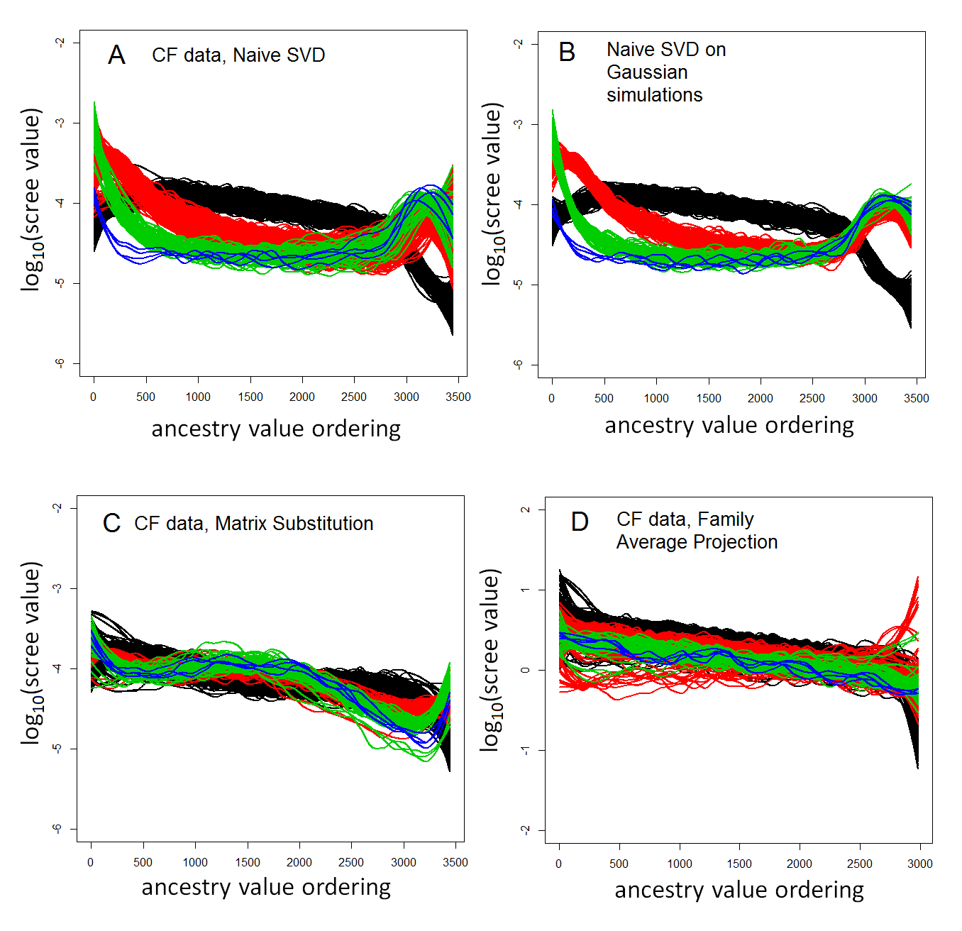
To carefully check these interpretations, we performed a simulation study using Gaussian data, with the approach described in the Supplement, and the numbers of each family type ($n_{f}=2,3,4$) matching the real CF data (panel B of Figure 6). The family patterns are very similar, although with somewhat less scatter, indicating that the geometric interpretations of these patterns are correct. Panel C shows the individual scree curves for matrix substitution, for which the curves of family members more closely overlap those of singletons. However, the curves for families of size 3 and 4 remain distinctive, as matrix substitution does not fully eliminate the effect of high correlation between family members. Panel D shows that the family average method achieves more general overlap of scree curves among the individuals.

Standard results for shared genotype probabilities for related individuals are expressed in terms of kinship coefficients and identity-by-descent probabilities. Here we clarify, as is needed for this paper, the correlation of genotypes between first-degree relatives. We focus on siblings, although a slight modification of the argument applies to parent-child relationships. Let $q$ denote the minor allele frequency, and a pair of siblings have random genotypes $g_{1}$ and $g_{2}$, with means $2q$ and variances $2q(1-q)$. We have

$\displaystyle corr(g_{1},g_{2})$

$\displaystyle=$

$\displaystyle\frac{E(g_{1}g_{2})-E(g_{1})E(g_{2})}{SD(g_{1})SD(g_{2})}=\frac{E(g_{1}g_{2})-(2q)^{2}}{2q(1-q)}.$

The identity-by-descent (IBD) outcomes determine $E(g_{1}g_{2})$. For IBD=0, $E(g_{1}g_{2}|IBD=0)=(2q)^{2}.$ Also, $E(g_{1}g_{2}|IBD=2)=E(g_{1}^{2})=2({\rm var}(g_{1})+E(g_{1})^{2})=2q(1-q)+(2q)^{2}.$ If IBD=1, without loss of generality, we assume the shared allele comes from the mother. We use $a_{m}$ to denote the allele from the mother and $a_{f}$ from the father. Then $E(g_{1}g_{2})=E((a_{m1}+a_{f1})(a_{m1}+a_{f2}))=E(a_{m1}^{2}+a_{f1}a_{m1}+a_{m1}a_{f2}+a_{f1}a_{f2})=q+3q^{2}.$ Therefore

	$\displaystyle E(g_{1}g_{2})$	$\displaystyle=$	$\displaystyle E(E(g_{1}g_{2}|IBD))$
		$\displaystyle=$	$\displaystyle\frac{1}{4}E(g_{1}g_{2}|IBD=0)+\frac{1}{2}E(g_{1}g_{2}|IBD=1)+\frac{1}{2}E(g_{1}g_{2}|IBD=2)$
		$\displaystyle=$	$\displaystyle\frac{1}{4}(2q)^{2}+\frac{1}{2}(2q(1-q)+(2q)^{2})+\frac{1}{4}(q+3q^{2})$

and plugging in to the correlation gives 0.5, regardless of $q$.

We have

$$AMA^{T}=\begin{bmatrix}I_{n-n_{\mathcal{F}}}&0^{T}\\ C^{T}&D^{T}\\ \end{bmatrix}\begin{bmatrix}M_{11}&M_{12}\\ M_{21}&M_{22}\\ \end{bmatrix}\begin{bmatrix}I_{n-n_{\mathcal{F}}}&C\\ 0&D\\ \end{bmatrix}$$

$$=\begin{bmatrix}M_{11}&M_{11}C+M_{12}D\\ C^{T}M_{11}+D^{T}M_{21}&\underbrace{C^{T}M_{11}C}_{a}+\underbrace{C^{T}M_{12}D}_{b}+\underbrace{D^{T}M_{21}C}_{c}+\underbrace{D^{T}M_{22}D}_{d}\\ \end{bmatrix}$$

$$=\begin{bmatrix}M_{11}&M_{12}\\ M_{21}&\tilde{M}_{22}\\ \end{bmatrix}.$$

Comparing the last two expressions provides two equations in the two unknowns $C$ and $D$. From the upper right, we have $M_{11}C+M_{12}D=M_{12}$, which implies $C=M_{11}^{-1}M_{12}(I_{2}-D)$ (the lower left is the same equation written in transpose form). The lower right requires a bit more effort. We consider each of the four terms separately, plugging in the solution for $C$ from above, giving

$$a=C^{T}M_{11}C=(M_{11}^{-1}M_{12}(I_{2}-D))^{T}M_{11}M_{11}^{-1}M_{12}(I_{2}-D)$$

$$=(I_{2}-D)^{T}M_{12}^{T}(M_{11}^{-1})^{T}M_{12}(I_{2}-D)=(I_{2}-D)^{T}S(I_{2}-D),$$

where $S=M_{12}^{T}(M_{11}^{-1})^{T}M_{12}=M_{21}M_{11}^{-1}M_{12}$.

$$b=C^{T}M_{12}D=(I_{2}-D)^{T}M_{12}^{T}(M_{11}^{-1})^{T}M_{12}D=(I_{2}-D)^{T}SD$$

$$c=D^{T}M_{21}C=D^{T}M_{21}M_{11}^{-1}M_{12}(I_{2}-D)=D^{T}S(I_{2}-D),$$

and $d$ does not simplify. We have

$$a+b+c+d=(I_{2}-D)^{T}S(I_{2}-D)+(I_{2}-D)^{T}SD+D^{T}S(I_{2}-D)+D^{T}M_{22}D=\tilde{M}_{22},$$

and the expression reduces to $D^{T}(M_{22}-S)D=\tilde{M}_{22}-S$. Thus, finally, we have our solution

$$C=M_{11}^{-1}M_{12}(I_{2}-D),~~D=(M_{22}-S)^{-1/2}(\tilde{M}_{22}-S)^{1/2}.$$

We simulated genotype data in a manner that respected local correlation structure, which is present but typically modest in SNPs used for stratification control, and reflected population ancestry. A SNP “block size” of 20 was chosen. An autoregressive normal model was used to simulate a set of modestly underlying correlated values, e.g. for one individual the value for the $i$th SNP is $Z_{i}=\rho Z_{i-1}+\epsilon$, where $\epsilon\sim N(0,1-\rho^{2})$, followed by reversal of sign of $\rho$ with probability 0.5. Marginally, each $Z_{i}\sim N(0,1)$, and a modest $\rho=0.2$ was used within each block and $\rho=0$ at block boundaries, so that values across different blocks were uncorrelated. To convert the values to genotypes, we first generated random minor allele frequencies by drawing “ancestral” allele frequencies from the half-triangular distribution $f(x)=2(x-a)/(a-b)^{2}$, where $a=0.38,b=0.50$, which corresponded closely to the observed minor allele frequency in the thinned CF dataset. For ancestral minor allele frequency $q$, the Balding-Nichols model was used for fixation index $F_{ST}$ by drawing $K$ subpopulation allele frequencies from the beta distribution with parameters $q(1-F_{ST})/F_{ST})$, and $(1-q)(1-F_{ST})/F_{ST}$. Conversion of the latent $Z$ values to genotypes was performed by applying, for each SNP and individuals in subpopulation $k$ with allele frequency $q_{k}$, an inverse quantile of ranked z-values such that the lowest $z$ values were converted to genotype 0, the largest to genotype 2, and genotypes 0, 1, and 2 occurred with frequencies $(1-q_{k})^{2}$, $2q_{k}(1-q_{k})$, and $q_{k}^{2}$ (i.e. Hardy-Weinberg equilibrium within each subpopulation $k$).

REFERENCES

- [2] [] Cabanski, C. R., Qi, Y., Yin, X., Bair, E., Hayward, M. C., Fan, C., Li, J., Wilkerson, M. D., Marron, J., Perou, C. M. et al. (2010), ‘Swiss made: Standardized within class sum of squares to evaluate methodologies and dataset elements’, PloS one 5(3), e9905.
- [4] [] Cattell, R. B. (1966), ‘The scree test for the number of factors’, Multivariate behavioral research 1(2), 245–276.
- [6] [] Conomos, M. P., Miller, M. B. & Thornton, T. A. (2015), ‘Robust inference of population structure for ancestry prediction and correction of stratification in the presence of relatedness’, Genetic epidemiology 39(4), 276–293.
- [8] [] Corvol, H., Blackman, S. M., Boëlle, P.-Y., Gallins, P. J., Pace, R. G., Stonebraker, J. R., Accurso, F. J., Clement, A., Collaco, J. M., Dang, H. et al. (2015), ‘Genome-wide association meta-analysis identifies five modifier loci of lung disease severity in cystic fibrosis’, Nature communications 6.
- [10] [] Epstein, M. P., Allen, A. S. & Satten, G. A. (2007), ‘A simple and improved correction for population stratification in case-control studies’, The American Journal of Human Genetics 80(5), 921–930.
- [12] [] Frudakis, T., Venkateswarlu, K., Thomas, M., Gaskin, Z., Ginjupalli, S., Gunturi, S., Ponnuswamy, V., Natarajan, S. & Nachimuthu, P. K. (2003), ‘A classifier for the snp-based inference of ancestry’, Journal of Forensic Sciences 48(4), 771–782.
- [14] [] Lake, S. L., Blacker, D. & Laird, N. M. (2000), ‘Family-based tests of association in the presence of linkage’, The American Journal of Human Genetics 67(6), 1515–1525.
- [16] [] Lee, S., Zou, F. & Wright, F. A. (2010), ‘Convergence and prediction of principal component scores in high-dimensional settings’, Annals of statistics 38(6), 3605.
- [18] [] Levine, D. M., Ek, W. E., Zhang, R., Liu, X., Onstad, L., Sather, C., Lao-Sirieix, P., Gammon, M. D., Corley, D. A., Shaheen, N. J. et al. (2013), ‘A genome-wide association study identifies new susceptibility loci for esophageal adenocarcinoma and barrett’s esophagus’, Nature genetics 45(12), 1487–1493.
- [20] [] Manichaikul, A., Mychaleckyj, J. C., Rich, S. S., Daly, K., Sale, M. & Chen, W.-M. (2010), ‘Robust relationship inference in genome-wide association studies’, Bioinformatics 26(22), 2867–2873.
- [22] [] Patterson, N., Price, A. L. & Reich, D. (2006), ‘Population structure and eigenanalysis’.
- [24] [] Price, A. L., Patterson, N. J., Plenge, R. M., Weinblatt, M. E., Shadick, N. A. & Reich, D. (2006), ‘Principal components analysis corrects for stratification in genome-wide association studies’, Nature genetics 38(8), 904–909.
- [26] [] Sankararaman, S., Sridhar, S., Kimmel, G. & Halperin, E. (2008), ‘Estimating local ancestry in admixed populations’, The American Journal of Human Genetics 82(2), 290–303.
- [28] [] Wright, F. A., Strug, L. J., Doshi, V. K., Commander, C. W., Blackman, S. M., Sun, L., Berthiaume, Y., Cutler, D., Cojocaru, A., Collaco, J. M. et al. (2011), ‘Genome-wide association and linkage identify modifier loci of lung disease severity in cystic fibrosis at 11p13 and 20q13. 2’, Nature genetics 43(6), 539–546.
- [30] [] Zhu, X., Li, S., Cooper, R. S. & Elston, R. C. (2008), ‘A unified association analysis approach for family and unrelated samples correcting for stratification’, The American Journal of Human Genetics 82(2), 352–365.