- 2D
- two-dimensional
- 3D
- three-dimensional
- AHRS
- attitude and heading reference system
- AUV
- autonomous underwater vehicle
- CPP
- Chinese Postman Problem
- DoF
- degree of freedom
- DVL
- Doppler velocity log
- FSM
- finite state machine
- IMU
- inertial measurement unit
- LBL
- Long Baseline
- MCM
- mine countermeasures
- MDP
- Markov decision process
- POMDP
- partially observable Markov decision process
- PRM
- Probabilistic Roadmap
- ROI
- region of interest
- ROS
- Robot Operating System
- ROV
- remotely operated vehicle
- RRT
- Rapidly-exploring Random Tree
- SLAM
- simultaneous localization and mapping
- SSE
- sum of squared errors
- STOMP
- Stochastic Trajectory Optimization for Motion Planning
- TRN
- Terrain-Relative Navigation
- UAV
- unmanned aerial vehicle
- USBL
- Ultra-Short Baseline
- IPP
- informative path planning
- FoV
- field of view
Online Informative Path Planning
for Active
Classification on UAVs
Abstract
We propose an IPP (IPP) algorithm for active classification using an UAV (UAV), focusing on weed detection in precision agriculture. We model the presence of weeds on farmland using an occupancy grid and generate plans according to information-theoretic objectives, enabling the UAV to gather data efficiently. We use a combination of global viewpoint selection and evolutionary optimization to refine the UAV’s trajectory in continuous space while satisfying dynamic constraints. We validate our approach in simulation by comparing against standard “lawnmower” coverage, and study the effects of varying objectives and optimization strategies. We plan to evaluate our algorithm on a real platform in the immediate future.


1 Introduction
Autonomous robots are increasingly used to gather information about the Earth’s ecosystems [6]. In agricultural monitoring, UAV are capable of providing high-resolution data in a flexible, cost-efficient manner [5]. Using sensors, UAV can survey crops to find precision treatment targets, improving yield and leading to sustainability and economic gain [2]. Unfortunately, UAV are often constrained by limited battery and computational capacities. Therefore, planning for efficient data collection is key in enabling robotics in this field.
We address the problem by proposing an IPP algorithm for active classification on a UAV equipped with an image-based weed classifier. We model the presence of weed on farmland using an occupancy grid. We continuously plan paths online through a combination of global viewpoint selection and evolutionary optimization, which refines the UAV’s trajectory in continuous 3D space while satisfying dynamic constraints. The resulting informative paths abide by a limited time budget and address the key challenge of trading off sensor resolution against coverage when flying at variable altitudes.
Our contributions are:
-
An IPP algorithm with the following properties:
- –
generates dynamically feasible trajectories in continuous space,
- –
obeys budget and sensing constraints,
- –
trades off sensor resolution against coverage in a principled manner by incorporating a height-dependent sensor noise model.
- –
-
An evolutionary strategy to optimize continuous UAV paths for maximum informativeness.
-
Validation of our approach in simulation against a coverage planner.
We plan to evaluate our algorithm in field experiments in the immediate future.
2 Related Work
Most previous IPP approaches seek to minimize map uncertainty using objectives derived from Shannon’s entropy [3, 13]. To exploit new data, adaptive approaches [11, 14, 8] replan paths based on specific interests. IPP can be performed using combinatorial optimization over a discrete grid [4, 12, 1]. However, the drawbacks of this representation are its limited scalability and resolution. Alternatively, some planners work in continuous space by leveraging sampling-based methods [13] or splines [3, 11, 15]. Similarly to Charrow et al. [3], we use global viewpoint selection to escape local minima and optimization to refine our trajectory.
IPP addressing UAV imaging is a relatively unexplored area. A set-up similar to ours has been studied recently by Sadat et al. [18]. However, their method assumes discrete viewpoints and prior knowledge of target regions, neglecting sensor noise. In contrast, our approach considers a height-dependent sensor model and incrementally replans as data are collected. Moreover, we use smooth polynomial trajectories which guarantee feasibility of the UAV’s dynamic constraints.
3 Problem Definition
We define the general IPP problem as follows. We seek a continuous path in the space of all possible paths for maximum gain in some information measure:
| (1) | ||||
where denotes a time budget and quantifies the objective, discussed in §4.3 for our application. The function measure(·) obtains measurements and time(·) provides the travel time along the path. Maximizing information gain rate, as opposed to maximizing only information, enables comparing the values of paths over different time scales.
4 Technical Approach
In this section, we present our IPP algorithm. The main idea is to create fixed-horizon plans maximizing an informative objective. To do this efficiently, we first select global viewpoints and then optimize the path in continuous space using an evolutionary method. In §4.1 and §4.2, we introduce our approaches to modeling and path parametrization. In §4.3, we detail our planning routine, shown in Alg. 1.
4.1 Environment and Measurement Models
We represent the environment (a farmland above which the UAV flies) using a 2D occupancy grid map [7], where each cell is associated with a Bernoulli random variable representing the probability of weed occupancy. For our measurement model, we assume a square footprint for a down-looking camera providing input to a weed classifier. The classifier provides probabilistic weed occupancy for cells within FoV (FoV) from a UAV configuration x. For each observed cell at time , we perform a log-likelihood update given an observation :
| (2) |
where the second term denotes the height-dependent sensor model capturing the weed classifier output. Our sensor model (Fig. 1, right) matches real datasets at low altitudes [10] and accounts for poorer classification performance with lower-resolution images taken at higher altitudes.
4.2 Path Parametrization
To create paths abiding by the dynamic constraints of the UAV, we connect viewpoints using the method of Richter et al. [17]. As in their work, we express a 12-degree polynomial trajectory in terms of end-point derivatives, allowing for efficient optimization in an unconstrained quadratic program.
4.3 Planning Algorithm
We use a fixed-horizon approach to plan adaptively. During the mission, we maintain viewpoints within a horizon H. We alternate plan execution and replanning, stopping when a time budget B is exceeded. For replanning, we adopt a two-stage approach consisting of global viewpoint selection and optimization. This procedure is described in Alg. 1 and illustrated in Fig. 2. The following sub-sections detail the key steps of Alg. 1.


Global Viewpoint Selection
In the first step (Lines 3-9), we sequentially select global measurement sites (Fig. 2(b)). Unlike in frontier-based exploration, common for indoor mapping [3], choosing viewpoints using map boundaries is not applicable in our set-up. Instead, we apply Eq. 1 over the horizon H (Line 2) to find most informative measurement sites. To find the next viewpoint efficiently, we evaluate the objective over a multiresolution lattice (Fig. 2(a)). To encourage exploration, we maximize entropy reduction in :
| (3) |
To encourage classification, we divide into “weed” and “non-weed” cells using thresholds and , leaving an unclassified subset . This is similar to finding unknown space in conventional occupancy mapping. We maximize the reduction of between time-steps:
| (4) |
We use an optional time-varying parameter (Line 3) to gradually bias viewpoint selection towards Eq. 4 from Eq. 3, focusing on weed identification over time. We then simulate a maximum likelihood (ML) measurement at (Line 7) and interpolate intermediate viewpoints to add degrees of freedom to the path (Line 9).
Optimization
In the second step (Line 10), we optimize the polynomial path by solving Eq. 1 in §3 using the Covariance Matrix Adaptation Evolution Strategy (CMA-ES). CMA-ES is a gradient-free optimizer suitable for continuous shape fitting with our discrete measurement model [9]. As evaluated in §5, we consider (i) globally optimizing (Fig. 2(c)) and (ii) optimizing only (Fig. 2(d)).
5 Results
Our algorithm is validated in simulation on 260 m environments with 120 Poisson-distributed weeds. We use thresholds of and , and use a replanning horizon of 7 viewpoints to limit optimization complexity. We initialize the UAV position as the map center with maximum altitude (45m). Our methods are evaluated against traditional “lawnmower” coverage with height fixed (8.66 m) for the same 300 s budget . We consider map entropy, classification rate, and mean F1-score as metrics, common for classification tasks. We simulate sensor noise using our model in §4.1. Following a similar approach to Pomerleau et al. [16], we compute the cumulative distribution function (CDF) of entropy over a time histogram to summarize variability among trajectories.
In our experiments, we study varying:
-
Optimization methods: no CMA-ES, local CMA-ES, global CMA-ES
As described in §4.3, for local CMA-ES, we consider optimizing to reduce inter-segment entropy. For global CMA-ES, we optimize , allowing points in to vote on the optimization objective for the entire trajectory.
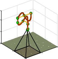
Fig. 3 compares the global viewpoint selection objectives with local CMA-ES optimization. Our methods outperform naïve coverage as they permit variable-altitude flight for wider FoV. As shown in Fig. 1, our planners usually produce paths similar to spirals, starting with descent to the unknown map center. The curves illustrate the coverage-resolution trade-off: for the classification objective (red curve), flying at low altitudes quickly provides accurate classification, as shown by the rises in classification rate and F1-score. However, entropy reduction is limited. By considering elapsed time when selecting global viewpoints (yellow curve), we obtain high certainty with efficient classification. Fig. 4 compares the CMA-ES optimization methods for the time-varying objective. The global method likely performs best due to the highest number of optimized variables.


6 Conclusion and Scheduled Experiments
We presented an adaptive IPP strategy for active weed classification on UAVs. Our algorithm combines global viewpoint selection with evolutionary optimization to generate dynamically feasible paths with informative objectives. We validated our strategy against a “lawnmower” coverage pattern and demonstrated the effects of using different objectives and optimization strategies.
We aim to implement our algorithm on an AscTec Neo UAV platform. Our experiments will take place at the ETH Lindau-Eschikon Research Station for Plant Sciences in Switzerland. We will consider active classification of crop-weed distributions on a 20-plot m sugarbeet field.
Acknowledgments.
This work was funded by the European Community’s Horizon 2020 programme under grant agreement no 644227-Flourish and from the Swiss State Secretariat for Education, Research and Innovation (SERI) under contract number 15.0029. We would like to thank the ETH Crop Science Group for providing the testing facilities.
References
- [1] Binney, J., Krause, A., Sukhatme, G.S.: Optimizing waypoints for monitoring spatiotemporal phenomena. IJRR 32(8), 873–888 (2013)
- [2] Cardina, J., Johnson, G.A., Sparrow, D.H.: The nature and consequence of weed spatial distribution. Weed Science 45(3), 364–373 (1997)
- [3] Charrow, B., Kahn, G., Patil, S., Liu, S., Goldberg, K., Abbeel, P., Michael, N., Kumar, V.: Information-Theoretic Planning with Trajectory Optimization for Dense 3D Mapping. In: Proc. RSS. pp. 3–12. Rome (2015)
- [4] Chekuri, C., Pál, M.: A Recursive Greedy Algorithm for Walks in Directed Graphs. In: Proc. IEEE FOCS. pp. 245–253 (2005)
- [5] Detweiler, C., Ore, J.P., Anthony, D., Elbaum, S., Burgin, A., Lorenz, A.: Bringing Unmanned Aerial Systems Closer to the Environment. Environmental Practice 17(3), 188–200 (2015)
- [6] Dunbabin, M., Marques, L.: Robots for environmental monitoring: Significant advancements and applications. IEEE Life Sciences 19(1), 24–39 (2012)
- [7] Elfes, A.: Using occupancy grids for mobile robot perception and navigation. Computer 22(6), 46–57 (1989)
- [8] Girdhar, Y., Dudek, G.: Modeling Curiosity in a Mobile Robot for Long-Term Autonomous Exploration and Monitoring. AURO 33(4), 645–657 (2015)
- [9] Hansen, N.: The CMA evolution strategy: A comparing review. Studies in Fuzziness and Soft Computing 192(2006), 75–102 (2006)
- [10] Haug, S., Ostermann, J.: A Crop / Weed Field Image Dataset for the Evaluation of Computer Vision Based Precision Agriculture Tasks. In: Proc. ECCV. pp. 105–116. Springer, Zürich (2014)
- [11] Hitz, G., Galceran, E., Garneau, M.È., Pomerleau, F., Siegwart, R.: Adaptive Continuous-Space Informative Path Planning for Online Environmental Monitoring. JFR (2016), under review
- [12] Hollinger, G., Singh, S., Djugash, J., Kehagias, A.: Efficient Multi-robot Search for a Moving Target. IJRR 28(2), 201–219 (2009)
- [13] Hollinger, G.A., Sukhatme, G.S.: Sampling-based robotic information gathering algorithms. IJRR 33(9), 1271–1287 (2014)
- [14] Lim, Z.W., Hsu, D., Lee, W.S.: Adaptive informative path planning in metric spaces. IJRR pp. 1–14 (2015)
- [15] Marchant, R., Ramos, F.: Bayesian Optimisation for Informative Continuous Path Planning. In: Proc. IEEE ICRA. pp. 6136–6143. Hong Kong (2014)
- [16] Pomerleau, F., Colas, F., Siegwart, R., Magnenat, S.: Comparing icp variants on real-world data sets. AURO 34(3), 133–148 (April 2013)
- [17] Richter, C., Bry, A., Roy, N.: Polynomial Trajectory Planning for Aggressive Quadrotor Flight in Dense Indoor Environments. In: Proc. ISRR. Springer, Singapore (2013)
- [18] Sadat, S.A., Wawerla, J., Vaughan, R.: Fractal Trajectories for Online Non-Uniform Aerial Coverage. In: Proc. IEEE ICRA. pp. 2971–2976. Seattle, WA (2015)