Blume-Capel ferromagnet driven by propagating and standing magnetic field wave: Dynamical modes and nonequilibrium phase transition
Muktish Acharyya1 and Ajay Halder2
Department of Physics, Presidency University
86/1 College street, Calcutta-700073, India
E-mail(1):muktish.physics@presiuniv.ac.in
E-mail(2):ajay.rs@presiuniv.ac.in
Abstract: The dynamical responses of Blume-Capel () ferromagnet to the plane propagating (with fixed frequency and wavelength) and standing magnetic field waves are studied separately in two dimensions by extensive Monte Carlo simulation. Depending on the values of temperature, amplitude of the propagating magnetic field and the strength of anisotropy, two different dynamical phases are observed. For a fixed value of anisotropy and the amplitude of the propagating magnetic field, the system undergoes a dynamical phase transition from a driven spin wave propagating phase to a pinned or spin frozen state as the system is cooled down. The time averaged magnetisation over a full cycle of the propagating magnetic field plays the role of the dynamic order parameter. A comprehensive phase diagram is plotted in the plane formed by the amplitude of the propagating wave and the temperature of the system. It is found that the phase boundary shrinks inward as the anisotropy increases. The phase boundary, in the plane described by the strength of the anisotropy and temperature, is also drawn. This phase boundary was observed to shrink inward as the field amplitude increases.
Keywords: Blume-Capel model, Monte Carlo simulation, Propagating wave, Standing wave, Dynamic Phase transition
I. Introduction:
Starting from its historical introduction, to analyse the thermodynamic behaviours of - transition in the mixture of He3 - He4, the Blume-Capel (BC) model[1, 2, 3] became an important model, mainly to study the bicritical/tricritical behaviours in various phase transitions. The low and high temperature series extrapolation techniques were employed[4] to determine the different (continuous and discontinuous) natures of the transition and hence the tricritical point (TCP) was found in the fcc BC ferromagnet. Monte Carlo study was performed[5] in fcc BC model and traced a phase boundary with tricritical point (TCP). Later, Monte Carlo (MC) simulation within microcanonical ensemble was studied[6] in Blume-Capel model to show the tricriticality. The critical behaviours of was studied[7]. It should be mentioned here that the variety of positional and/or orientational order and a very rich phase diagram was obtained[8] recently even in Ising system in three dimensions by renormalization group theory in Migdal-Kadanoff approximation. The general spin BC model was studied[9] by meanfield approximation. The meanfield solution was obtained[10] in BC model with random crystal field. Effects of random crystal field in BC model was studied[11] by effective field theory. The wetting transition in BC model was studied[12] by MC simulation.
Interestingly, the BC model exhibits the competing metastability which has an important role in its dynamical behaviours. In this context, it should be mentioned that dynamic Monte Carlo and numerical transfer matrix method [13] were employed to study the competing behaviours of the metastability in the BC model. The behaviours of the competing metasatble states at infinite volume are studied [14] in dynamic BC model. The metastable and unstable states are obtained [15] by cluster variation and path probability method.
The researchers paid attention to study the nonequilibrium behaviours (in the presence of time varying magnetic field) of Ising[16], Heisenberg[17] and BC model. The nonequilibrium dynamic phase transition was studied[18] in BC model in the presence of an oscillating (in time but uniform over space) by effective field analysis and Glauber dynamic approach. The nonequilibrium dynamics was studied[19] in BC model with quenched random fields. The effective field theory was developed[20] for kinetic BC model driven by oscillating magnetic field to study the dynamic phase transition. The meanfield approach was employed [21] to study the dynamic phase transition in Glauber kinetic spin-1 blume-Capel model swept by oscillating magnetic field.
What kind of nonequilibrium responses and the transitions are expected if the Blume-Capel ferromagnet is swept by propagating and standing magnetic wave ? The above mentioned nonequilibrium responses are due to an oscillating magnetic field which is oscillating in time but uniform over the space. The system will respond differently if the externally applied field has spatio-temporal variation. The nonequilibrium responses of the Ising ferromagnet were recently studied by applying propagating magnetic field wave and various interesting spin wave motion and nonequilibrium phase transitions are observed[22, 23, 24]. The dynamic phase transitions, in the Ising ferromagnet, are studied recently [25] in the presence of standing magnetic field wave.
In this paper, the nonequilibrium responses of Blume-Capel ferromagnet () are studied in the presence of propagating and standing magnetic field wave by Monte Carlo simulation. The paper is organized as follows: the model is described in the section II, the numerical results are reported in section III and the paper ends with summary in section IV.
II. Model and simulation:
The energy of the two dimensional Blume-Capel ferromagnet in the presence of magnetic field (having spatio-temporal variation) is
| (1) |
where, represents the z component of the Spin () at any position () in time . The values of may be any one of -1,0 and +1. is the uniform (over the space) ferromagnetic interaction strength. The first term represents the ferromagnetic nearest neighbour spin-spin interaction. The second term provides the contribution due to the anisotropy (). The last term represents the interaction between spin and the externally applied magnetic field having spatio-temporal variation. denotes the value of magnetic field at position at time . Two types of the forms of are chosen here e.g., propagating wave and standing wave. The propagating magnetic field wave is represented as
| (2) |
The standing magnetic field wave may be represented as
| (3) |
For simplicity, the magnetic field wave, considered here, is propagating in the direction. The , and represent the amplitude, frequency and the wavelength of the magnetic field waves (both propagating and standing) respectively. The periodic boundary conditions are applied in both directions of the square lattice to preserve the translational invariances in the system.
III. Results:
(i) For propagating wave
In this study, a square lattice of size is considered. The system is driven by a propagating (moves in the direction) magnetic field wave having fixed wavelength and frequency . The frequency and wavelength of the propagating magnetic field wave are kept constant throughout the study. The system () contains two full waves for this choice of particular value of . Initially, a high temperature ( here) random phase is considered where the system is prepared with a random uniform distribution of the values (1, 0, and -1) of . This is a high temperature paramagnetic phase. Now the system is slowly (with decrement of temperature equals to 0.02) cooled to achieve the nonequilibrium steady state at any fixed temperature . In this Monte Carlo simulation, the Metropolis single spin flip algorithm with parallel updating[26] rule is employed. The probability of spin flip is chosen as , where, is energy required for spin flip and is the Boltzmann constant. The field amplitude () and the strength of anisotropy () are measured in the unit of and the temperature are measured in the unit of . such updating of spins defines the unit of time i.e., Monte Carlo step per spin (MCSS) here. At any temperature, the system is allowed to pass through MCSS and initial (or transient) MCSS are discarded. The dynamical quantities are calculated over MCSS. It may be noted here, that for frequency of the propagating magnetic field wave, 100 MCSS is required to have a complete cycle of the propagating magnetic field wave. So, in MCSS, 500 such cycles of the propagating magnetic field are present. It is checked that this length of simulation is adequate to achieve the nonequilibrium steady state. The instantaneous magnetisation is , the time averaged magnetisation over the full cycle of the propagating magnetic field is . Due to the intrinsic stochasticity in the Metropolis dynamics, the values of are different in different cycles. As a result, has a statistical distribution. The variance of is , where is average of over 500 different values of . It is checked that this number of samples is sufficient to have good statistics.
It is found that, for fixed values of and , two different dynamical phases are identified. In the high temperature, two distinct and alternate bands of spin values and are formed. They are found to propagate. A few sites having are found along the boundary of the bands. For sufficiently high values of the temperature () of the system and the amplitude () of the propagating magnetic field, these spin-bands are observed to be propagating coherently along the direction of propagation of the magnetic field wave. One such coherent propagation of spin-wave is shown in Figure-1. It should be mentioned that the term spin-wave used here is strictly different from the conventional notion of spin-wave in condensed matter physics.
The low temperature dynamical phase is not the coherent propagation of spin-waves. For fixed values of and as the system is cooled down, the system transits to a different phase. This is a spin-frozen or pinned phase, where most of the spins are pinned or frozen to any one value of . Here, the propagating magnetic field wave does not have any effect on the spins of the system. The spin flip is almost stopped in this phase. The two major dynamical phases are observed, namely, the high temperature spin-wave propagating phase and low temperature spin-frozen or pinned phase. In the spin-wave propagating phase, the populations of depends on the value of the strength of anisotropy . For lower values of , this population increases. The dependences of these dynamical phases on , and are shown in a comprehensive manner in Figure-2. It may be noted here that the dynamical phase transition was studied [24] also in Ising ferromagnet swept by propagating magnetic field. A similar coherent propagation of spin bands was observed there. However, in the Blume-Capel ferromagnet, in the low temperature () and high field () propagating phase, the large population of was observed in the interfacial region of spin bands formed by and (see Fig-2(iii)).
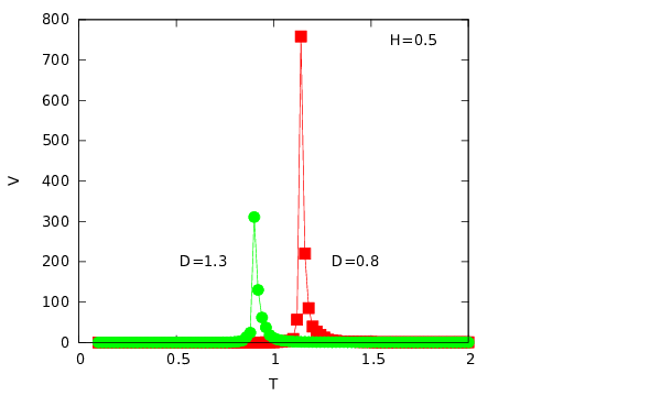
To study the dynamical phase transition quantitatively, the dynamical order parameter and its variance are studied as a function of temperature with and as parameters. For fixed value of and , in the high temperature spin-wave propagating phase, the dynamical order parameter assumes zero value and in the low temperature region, becomes nonzero. Actually, modulus of is greater than zero in the low temperature spin-frozen phase. As the system is cooled down it undergoes a dynamical phase transition from a spin-wave propagating phase to a spin-frozen phase. The order parameter starts to assume a nonzero value at any finite temperature which gives rise to a dynamical phase transition. From the temperature dependence of , the transition seems to be continuous. This dynamical phase transition is also detected from the temperature variation of , which shows a very sharp peak at the transition temperature. It is believed to diverge eventually in the limit. A typical such variation is shown in Figure-3. In this figure, the dependences of the transition temperature on , is also shown. For a fixed value of , the transition occurs at lower temperature as one increase the strength of anisotropy . As an example, here for the peaks of are observed at and for and respectively. For lower value of anisotropy () the dynamic transitions occur at and for and respectively, indicated by the sharp peaks on .
This dynamical phase transition detected jointly from the temperature dependences of and is found to be happened at lower temperature as one increase the amplitude () of the propagating magnetic field wave keeping all other parameters fixed. For any fixed value of just by getting the transition temperature (from the peak position of ) as a function of , the comprehensive dynamical phase boundary (in the plane formed by and ) is obtained and shown in Figure-4. The phase boundary is observed to shrink inward (lower values of and ) as the strength of anisotropy increases. The transitions observed, along the entire phase boundary, are of continuous types. It may be noted here that the equilibrium transition temperature (for , ) is very close to 1.8 (see Fig-2 of Ref[12]). The results for , obtained here, may be compared to that.
The variances of is studied as function of temperature for two different values of (with fixed ). This shows the transition occurs at lower temperature for higher values of . These are shown in Figure-5. As an example here, for the transitions occur at and for and respectively. Similarly, for the transitions occur at and for and respectively.
In a similar method, the dynamical phase boundaries are obtained and sketched in the plane formed by and for two different values of . It is shown in Figure-6. It is observed that for large values of , the phase boundary shrinks inward (lower values of and ). Here also, along the entire phase boundary, the dynamical transitions are found to be continuous.
(ii) For Standing wave
The dynamical phase transition was studied also in Blume-Capel ferromagnet irradiated by standing magnetic wave. Here the frequency of the standing wave is chosen and the wavelength was taken . These choice of and are kept fixed throughout the study.
Here also, like the case of propagating wave, two distinctly different dynamical modes were observed. For a fixed set of values of and , the low temperature phase is a spin-frozen state and the high temperature phase shows the formation of alternate ( and ) spin bands. These spin bands does not propagate. The spin bands also form a standing spin-waves. To be precise, as the system is cooled down from a high temperature, the system undergoes a nonequilibrium phase transition from a standing spin-wave phase to a spin frozen phase. These typical morphologies are shown in Figure-7. It may be noted here, that similar standing spin bands were observed [25] in the case of Ising ferromagnet swept by standing magnetic wave. Here, no interfacial population of was observed unlike case of propagating wave (applied in BC model).
To distinguish the propagating spin wave and the standing spin wave phases the snap shots of the spin configurations of the lattice are shown for a fixed set of values of , and at two different times (MCSS and MCSS). This is shown in Figure-8. No signature of propagation of the alternate spin bands was observed. Reader may compare this with Figure-1, where the coherent propagation of spin bands was observed with the application of external propagating magnetic field wave.
The temperature dependences of and are studied using and as parameter and shown in Figure-9. The sharp peaks of indicated the transition temperature of the nonequilibrium phase transition from high temperature standing spin wave to low temperature spin frozen state. The transition temperatures are found to depend on and . This is comprehensively shown in the Table-I.
| H | D | |
|---|---|---|
| 0.50 | 0.10 | 1.50 |
| 0.50 | 0.50 | 1.38 |
| 1.00 | 0.10 | 1.20 |
| 1.00 | 0.50 | 1.10 |
The comprehensive phase boundaries in the H-T plane are plotted in different values of D and shown in Figure-10. The phase boundary was found to shrink inward (lower values of and ) as D increases. The transition was observed to be continuous through the entire phase boundary.
The nonequilibrium phase transitions with application of standing magnetic wave are studied in the plane described by D and T (for different values of H). The comprehensive phase boundaries in the D-T plane are plotted and shown in Figure-11. Here also, the phase boundary was observed to shrink inward (lower values of D and T) as H increases. The nature of the transition remains continuous through the entire phase boundary.
We have compared a phase diagram (for standing wave and ) of dynamic phase transition with that obtained from a meanfield study [21] of Glauber kinetic BC model. The results are shown (Figure-12) in a plot of suitably rescaled temperature () and field amplitude (). The variable represents the coordination number which is equal to 4 in the case of a square lattice (in this study).
IV. Summary:
The dynamics of the Blume-Capel (S=1) ferromagnet in the presence of the plane propagating and standing magnetic field waves are studied in two dimensions by Monte Carlo simulation. The Metropolis single spin flip algorithm with parallel spin updating rule are used. The different dynamical states of the system are observed to depend on the values of the strength of anisotropy, temperature of the system and the amplitude of the plane magnetic field waves (both propagating and standing). Here, mainly two different dynamical phases are observed. For a fixed value of anisotropy and the amplitude of the propagating magnetic field, the system undergoes a dynamical phase transition from a driven propagating spin wave phase to a pinned or spin frozen state as the system is cooled down. In the driven spin wave state, the coherent motion of the alternate spin-bands of and are found.
The time averaged magnetisation over a full cycle of the propagating magnetic field plays the role of the dynamic order parameter. Accordingly, the spin frozen or pinned phase is characterised by nonzero value of the dynamical order parameter. The dynamical order parameter becomes zero in the phase of coherent propagation of the spin-bands. This dynamical order parameter takes a nonzero value at the transition temperature as the system is cooled down. The variance of the order parameter gets sharply peaked at the transition point. The transition temperature is found from the peak position of the variance of the dynamic order parameter. This dynamic transition temperature was found to be function of amplitude of the propagating magnetic field wave and the strength of the anisotropy. A comprehensive phase diagram is plotted in the plane formed by the amplitude of the propagating wave and the temperature of the system. It is found that the phase boundary shrinks inward (lower temperature) as the strength of the anisotropy increases. The phase boundary, in the plane described by the strength of anisotropy and temperature, is also drawn. Here, this phase boundary was observed to shrink inward as the amplitude of the propagating magnetic field wave increases.
The dynamical responses of the Blume-Capel model was studied here with the application of standing magnetic wave. Here, the high temperature phase is quite different from that observed in the case of propagating magnetic wave. The standing wave (non propagating) of alternate spin bands are formed. The dynamical phase boundaries are plotted in the H-T and D-T planes. The qualitative behaviours are same as observed in the case of propagating magnetic wave.
It may be noted that the sharp peak of the variance at the transition point is a signature of the divergence (in the thermodynamic limit) of the dynamic susceptibility. The Blume-Capel model shows tricritical behaviour in the equilibrium phase transition. However, in this particular nonequilibrium case, the transition seems to be continuous irrespective of the value of the strength of the anisotropy.
A qualitative understanding of the existence of the dynamical phases may be as follows: at low temperature the values D and H are inadequate for spin flip. As a result one obtains the spin frozen phase. On the other hand if the temperature is high the same set of values of D and H become strong enough to flip the spins. In this phase spins are flexible enough to respond to the variation of propagating and standing magnetic wave. As a result, the propagating magnetic wave yields propagating spin bands and standing magnetic wave produces standing spin bands in the lattice. Phase boundaries is nothing but the dependences of the dynamic transition temperature on the values of D and H.
Recently, the site diluted BC model was studied[27] by meanfield renormalization group analysis with good agreement of the experimental phase diagram of Fe-Al alloy. The magnetic alloy of Fe-Al can be modelled by Blume Capel ferromagnet and it would be interesting to see the coherent propagation of spin-bands and the standing spin band experimentally by time resolved magneto-optic Kerr (TRMOKE) effect. This study has a significance in the field of spintronics and magnonics[28]
The magnetic behaviours of core-shell magnetic nanoparticles has an important in the magnetism research as well as in the technology. The magnetic properties have been studied[29] in bimagnetic () core-shell nanoparticles. The dynamical phase transition has been studied [30] by Monte Carlo simulation in spherical core-shell ( core and shell) under time dependent (uniform over space) magnetic field. It would be interesting to study the dynamical behaviours of core-shell magnetic nanoparticles in presence of a magnetic field having spatio-temporal variation appearing as magnetic propagating wave, standing wave etc.
References
References
- [1] M. Blume, Phys. Rev. 141 (1966) 517
- [2] H. Capel, Physica. 32 (1966) 966
- [3] M. Blume, V. J. Emery and R. B. Griffith, Phys. Rev. A 4 (1971) 1071
- [4] D. M. Saul, M. Wortis and D. Stauffer, Phys. Rev. B. 9 (1974) 4964
- [5] A. K. Jain and D. P. Landau, Phys. Rev. B, 22 (1980) 445
- [6] M. Deserno, Phys. Rev. E, 56 (1997) 5204
- [7] J. C. Xavier, F. C. Alcaraz, D. P. Lara, J. A. Plascak, Phys. Rev. E 57 (1998) 11575
- [8] C. Yunus, B. Renklioglu, M. Keskin and A. N. Berker, Phys. Rev. E, 93 (2016) 062113
- [9] J. A. Plascak, J. G. Moreira, F. C. saBarreto, Phys. Lett. A. 173 (1993) 360
- [10] P. V. Santos, F. A. de Costa, J. M. de Araujo, Phys. Lett. A, 379 (2015) 1397
- [11] Y. Yuksel, U. Akinci, H. Polat, Physica A 391 (2012) 2819
- [12] E. V. Albano and K. Binder, Phys. Rev. E 85 (2012) 061601
- [13] T. Fiig, B. M. Gorman, P. A. Rikvold and M. A. Novotny, Phys. Rev. E 50 (1994) 1930
- [14] F. Manzo and E. Olivieri, J. Stat. Phys. 104 (2001) 1029
- [15] C. Ekiz, M. Keskin and O. Yalcin, Physica A 293 (2001) 215
- [16] B. K. Chakrabarti and M. Acharyya, Rev. Mod. Phys. 71 (1999) 847
- [17] M. Acharyya, Int. J. Mod. Phys. C 16 (2005) 1631.
- [18] M. Ertas, M. Keskin and B. Deviren, J. Magn. Magn. Mater. , 324 (2012) 1503
- [19] E. Vatansever and H. Polat, J. Magn. Magn. Mater. , 332 (2013) 28
- [20] M. Ertas, Y. Kokakaplan, M. Keskin, J. Magn. Magn. Mater. , 348 (2013) 113
- [21] M. Keskin, O. Canko and U. Temizer, Phys. Rev. E, 72 (2005) 036125
- [22] M. Acharyya, J. Magn. Magn. Mater. 354 (2014) 349
- [23] M. Acharyya, J. Magn. Magn. Mater. 382 (2015) 206
- [24] M. Acharyya, Acta Physica Polonica B, 45 (2014) 1027
- [25] A. Halder and M. Acharyya, J. Magn. Magn. Mater. 420 (2016) 290
- [26] K. Binder and D. W. Heermann, Monte Carlo simulation in statistical physics, Springer series in solid state sciences, Springer, New-York, 1997
- [27] D. Das and J. A. Plascak, Phys. Lett. A 375 (2011) 2089
- [28] S. Bader and S. S. P. Parkin, Annu. Rev. Condens. Matter Phys. 1 (2010) 71-88
- [29] H. Zeng, S. Sun, J. Li, Z. L. Wang and J. P. Liu, Applied Physics Letters, 85 (2004) 792
- [30] E. Vatansever and H. Polat, J. Magn. Magn. Mater. 343 (2013) 221

|

|


|


|


|


|

|

|
|

|

|

|

|

|

|

|

|

|

|