Data Sketching for Large-Scale Kalman Filtering
Abstract
In an age of exponentially increasing data generation, performing inference tasks by utilizing the available information in its entirety is not always an affordable option. The present paper puts forth approaches to render tracking of large-scale dynamic processes via a Kalman filter affordable, by processing a reduced number of data. Three distinct methods are introduced for reducing the number of data involved in the correction step of the filter. Towards this goal, the first two methods employ random projections and innovation-based censoring to effect dimensionality reduction and measurement selection respectively. The third method achieves reduced complexity by leveraging sequential processing of observations and selecting a few informative updates based on an information-theoretic metric. Simulations on synthetic data, compare the proposed methods with competing alternatives, and corroborate their efficacy in terms of estimation accuracy over complexity reduction. Finally, monitoring large networks is considered as an application domain, with the proposed methods tested on Kronecker graphs to evaluate their efficiency in tracking traffic matrices and time-varying link costs.
Index Terms:
tracking, dimensionality reduction, censoring, random projections, Kalman filter, traffic matrix.I Introduction
Tracking nonstationary dynamic processes is of paramount importance in various applications. In the context of big data, being able to perform accurate and economical state estimation may render problems of prohibitive scale feasible. Weather prediction is an example of tracking a slowly-varying dynamic process, from a massive volume of observations acquired from fast-sampling sensors per time interval; see e.g., [1]. Monitoring large and dynamically evolving networks, where nodes may join or leave and connections may be established or lost as time progresses, provides an exciting domain in which the acquisition and processing of network-wide performance metrics becomes challenging as the network size increases [2, Ch. 8]. For instance, monitoring path metrics such as delays or loss rates is challenging primarily because the number of paths generally grows as the square of the number of nodes in the network. Therefore, measuring and storing the delays of all possible origin-destination pairs is hard in practice, even for moderate-size networks [2].
In this context, efforts to reduce the number of measurements used for tracking have pursued two different directions. The first is that of optimal experimental design (OED), where the goal is to perform model-driven sensor selection based on ensemble performance metrics (e.g. the trace of the error covariance). Channel-aware dimensionality reduction of observations was reported in [3] and [4] using distributed wireless sensor networks (WSNs). Optimal and near optimal sensor schedules for a finite time horizon estimation was dealt with in [5], while entropy- and mutual-information-based sensor selection were advocated in [6] and [7]. A posterior-CRLB-based method to select sensors for tracking was introduced in [8], via convex optimization in [9] and [10], while a greedy algorithm leveraging submodularity was developed in [11] for measurement selection in sequential estimation. The latter has also been advocated as a means of reducing the complexity of Kalman filters that operate with limited processing resources [12]. OED is nicely attuned for designing low-dimensional observation models, but it is data-agnostic and thus sub-optimal when observations become available and need to be reduced.
The second direction is that of data-driven methods that select available measurements for processing. Specifically, censoring has recently been employed to select data for distributed parameter estimation using resource-constrained WSNs, thus trading off performance for tractability [13, 14]. Furthermore, censoring has been proposed for signal estimation using WSNs, for tracking, and control of dynamical processes [15, 16, 17, 18]. However, existing works on censoring mainly aim at reducing the rate at which sensors communicate their observations, and pertinent methods exhibit large computational complexity and storage requirements, which can be possibly afforded only at the fusion center.
The goal of this paper is to perform reliable tracking using the Kalman filter (KF), while reducing the amount of data and the computational complexity involved. To this end, the first two methods employ random projections and innovation-based censoring to respectively effect dimensionality reduction and measurement selection. The third method reduces complexity by leveraging sequential processing of observations when the noise is uncorrelated, and by selecting a few informative updates based on an information-theoretic metric. Finally, an efficient backward smoothing method is developed to mitigate the performance degradation caused by dimensionality reduction. Corroborating simulations compare with state-of-the-art greedy measurement selection algorithms, and illustrate the efficacy of the novel schemes. To demonstrate the applicability of the proposed update selection approach on real-world problems, traffic matrix estimation and network link cost estimation is also considered.
The rest of the paper is organized as follows. Section II introduces the proposed model of reduced complexity KF. Sections III and IV present the two dimensionality reduction modules based on RPs and censoring, respectively. The proposed update selection method is introduced in Section V. Numerical experiments are in Section VII, while Section VIII includes experiments on network monitoring. Finally, concluding remarks are given in Section IX.
Notation. Lower- (upper-) case boldface letters denote column vectors (matrices). Calligraphic symbols are reserved for sets, while T stands for transposition. Vectors , , and denote the all-zeros, the all-ones, and the -th canonical vector, respectively. Symbol denotes the indicator for the event . Notation stands for the multivariate Gaussian distribution with mean and covariance matrix , while , , and are reserved for the trace, the minimum and maximum eigenvalues of matrix , respectively. Symbol is used to denote that the number of observations is “prohibitively large” relative to the problem at hand, as well as the computing platform.
II Problem Statement and Preliminaries
Consider the following linear dynamical system model
| (1) | ||||
| (2) |
where denotes the state vector at time ; is the known state-transition matrix; and are known, deterministic control-input model and control-input vector respectively; the measurement vector, and is the known measurement matrix; while and are zero-mean, mutually uncorrelated and individually uncorrelated across time random noise vectors, with respective covariance matrices and . The initial state has mean , and covariance .

Given the information-bearing data of the measurement (2) at time , the most recent estimate and its covariance matrix , the celebrated KF yields the minimum mean-square error (MMS- E) optimal estimate in two steps. First, the state prediction and its covariance matrix are obtained using the model dynamics as [cf. (1)]
Subsequently, as becomes available, is obtained as
| (4) |
The first term of the cost in (4) is a weighted least-squares term fitting the state with that arises from the linear observation model in (2); while the second regularization term corresponds to treating as a prior of . Solving (4) and applying the matrix inversion lemma (MIL) yields the well known KF correction step, e.g., [19, p. 205]
where the so-termed KF gain and the state covariance update are given by
A dual form of the KF known as the information filter (IF) relies on the MIL to offer a more efficient solver of (4) as grows large [19, Ch. 7]. Nevertheless, even the low-complexity IF requires multiplications to solve (4) in the case of uncorrelated observations ( diagonal), and in general. Therefore, for large-scale KF problems where , dimensionality reduction of the datasets is well motivated for rendering the solution of (4) computationally tractable, while also reducing other data-related costs, such as storage and transmission.
Towards this goal, we introduce a reduced-complexity Kalman-like filter (see Algorithm 1) that extracts a reduced (size ), yet informative dataset from the original , where and are the corresponding reduced-dimension observation vector, measurement matrix, and covariance matrix; see also Fig. 1. Consequently, the problem reduces to the design of low-complexity sketching modules for informative dimensionality reduction. In the ensuing two sections, a data-agnostic method based on RPs followed by a data-adaptive method based on censoring are developed.
III RP-based KF
RP-based dimensionality reduction amounts to premultiplying measurements and regressors with a random matrix , and a diagonal matrix , whose entries take the values equiprobably. The net result is a linear transformation of the measurement equations so that all rows convey “comparable information”. A subset of rows of the transformed system is then extracted by simple random sampling, implemented by left multiplication with a random selection matrix .
Originally developed for linear regressions [20, 21, 22], the novelty here is RP-based reduced-dimensionality tracking of dynamical processes. Applying the Hadamard preconditioning and random sampling matrices on (2) yields the reduced-dimension observation model
where is zero mean with covariance . Given and the reduced data , state estimate can be obtained as [cf. (4)]
| (5) |
Solving (5) and applying the MIL yields the novel RP-based KF, which is summarized as Algorithm 1 using Algorithm 2 as sketching module.
Implementing RPs can have affordable complexity if is chosen to be a pseudo-random Hadamard matrix of size for . Different from the more elaborate approaches in [3] and [4], the proposed RP-KF is an easy-to-implement, “one-size-fits-all” reduced-complexity tracker, using data-agnostic dimensionality reduction. Furthermore, RP-KF’s estimation performance can be guaranteed as asserted in the ensuing proposition, which provides a benchmark for the data-driven methods introduced in the following section.
Proposition 1.
With , let , , and the singular value decomposition of . If for some , then by choosing the following bound for the RP-KF estimates holds w.h.p.
where denotes the condition number of , and is the full-data KF estimate.
Proof.
See Appendix 1. ∎
Proposition 1 asserts that, per time slot , the estimate of the RP-KF can be guaranteed to be close enough, in the relative squared-error sense, to the estimate of the full KF, if the reduced dimension is chosen to be large enough. Note that Proposition 1 only provides a per-step error guarantee, meaning that the error between the estimates of the RP-KF and the full-data KF at slot is bounded, given that the two filters share a common estimate at slot . Bounding the RP-KF error across multiple time slots is a more challenging task that goes beyond the scope and claims of the present paper. Naturally, the quality of the approximation also depends on other parameters such as the observation matrix, noise variance and covariance of prediction. Nevertheless, being data-agnostic and requiring storage and processing of in batch form per time slot renders the RP-KF less attractive in practice, and motivates the algorithms presented in the following two sections.
IV CENSORING-BASED KF
Measurement censoring for estimating dynamical processes has been advocated as a means of reducing the inter-sensor transmission overhead when WSNs are deployed for distributed tracking [16, 17]; see also [15, 23], where censoring is employed for event-based estimation. Since the goal in the aforementioned applications is saving communication resources, censoring is performed solely on measurements , with and assumed known and used even for the censored entries of ; thus, [16, 15, 23, 14], and [17] rely on reducing the dimensionality of a dataset that only consists of observations; that is, . A subset of observations is obtained, where is the th entry of , and denotes a set collecting the indices of uncensored observations. Given and , [16, 15, 23, 14, 17] develop sequential estimators to optimally estimate . Targeting reduction of communication load, optimal (in the maximum likelihood or MMSE sense) estimation from (un)censored observations comes with complexity comparable to that of using the full set of measurements. For our big-data setups, this is not affordable.
Since the aim is dimensionality and complexity reduction, the starting point is on censoring entire rows of the full dataset , in order to obtain a reduced set , where denotes the th row of and . The goal here is to develop censoring rules in order to obtain , so that is an “informative” subset of . Most existing censoring schemes adopt the innovation as a measure of information contained in .
One approach –henceforth termed block censoring (BC)– is to censor the entire vector . From an information-theoretic viewpoint [17], the optimal BC rule relies on the magnitude of the prewhitened innovation , where ; thus, is found as
Clearly, having corresponds to skipping the correction step of the KF. A major shortcoming of (IV) is the cubic complexity associated with inverting . Furthermore, BC-KF can only reduce the data cost on average across iterations by entirely skipping correction steps.
Our idea of a more attractive alternative is to possibly censor separately each entry of . Such an entry-wise censoring rule yields as
| (8) |
where , and can be tuned so that the set cardinality . Note that normalization in (6) includes pre-whitening of the innovation vector that is effected through left multiplication with . In contrast, any low-complexity per-entry adaptive censoring rule cannot explicitly consider the cross-correlation between different measurements, meaning that is not utilized. Instead, (8) uses the diagonal entries of as an approximate measure of the per-entry innovation variance and therefore it serves as a normalization factor. Compared to BC-KF, the innovation-based entry-wise rule of (8) is more flexible in reducing the available data, since it can censor any subset of observations at slot at much lower complexity. Nevertheless, to accurately perform measurement selection with (8), must reflect how informative is for the purpose of tracking . Using for this purpose the entry-wise predictor-based innovations is a possibility, but turns out to be unsuitable for the proposed reduced-complexity KF, due to the fact that censoring rule (8) tends to yield “biased” observations for a given . Correction of this bias is possible through the incorporation of a maximum likelihood criterion (see, e.g. [24]). Since such an approach requires the additional knowledge of and incurs computational complexity at least as high as that of the full-data KF, it is only suitable for reducing the communication overhead.
Targeting a more suitable censoring rule, the adaptive censoring least mean-square (AC-LMS) algorithm we introduced in [24] for non-dynamical regressions can be employed to discard uninformative rows of . Within time slot , rows of are processed sequentially; given a temporary estimate , the th row is discarded when indicated so by the censoring variable ( denotes the indicator function)
| (9) |
Given , a “censoring slab” is specified in to determine whether will be censored (if inside this slab) or not (if outside this slab). If deemed informative enough , the th row is added to , and subsequently involved in updating as
| (10) |
The role of the first-order update in (10) is to perturb the censoring slab towards the direction of , thus making it less likely for future measurements conveying information “close to” to be retained. Intuitively speaking, such updates eliminate measurement redundancies and reduce estimation error due to the bias of uncensored observations. The AC sketching module is summarized as Algorithm 3, and when plugged into Algorithm 1, it yields the proposed adaptive censoring (AC)-KF scheme. With regards to its performance, we have the following result.
Proposition 2.
If , , and , are zero-mean Gaussian, then the AC-KF with yields unbiased estimates .
Proof.
See Appendix 3. ∎
The assumptions in Proposition 2 were made to simplify the proof and are not necessary. Extensive simulations indicate that the AC-KF remains unbiased even for low and correlated noise, and also for . Nevertheless, the variance of AC-KF largely depends on the choice of . Tuning to optimize the MSE performance of AC-KF is a challenging task. Accurate rules for selecting is part of our ongoing research. However, even for possibly suboptimal values of , the proposed scheme yields promising results. Simulations in Section VII will demonstrate that the proposed AC-KF attains estimation accuracy close to that of the KF using the greedy measurement selection method in [11]. In addition, the proposed sketching module performs a single pass over the data, and requires computations, which is markedly lower than the required to perform greedy selection. Furthermore, AC-KF is suitable for online implementation by processing rows of sequentially. Table I summarizes the per-slot computational complexity of applying the sketching modules corresponding to AC-KF, RP-KF and random sampling.
Remark 1: Note that (9) does not pertain to a filter update. Instead, it is an update of within the AC sketching module (Algorithm 3) that leverages uncensored entries per slot, and it is only used for censoring entries within of slot . Note also that for Algorithm 3 performs adaptive censoring on . If , then , and thus the censoring rule in (8) becomes non-adaptive across measurements at slot . For AC-KF with non-adaptive censoring, scalar entries of the measurement vector can also be censored in a decentralized fashion across distributed sensors.
| Sketching method | Complexity |
|---|---|
| Random sampling | |
| Random projections (RP-KF) | |
| Adaptive censoring (AC-KF) |
V Update-Selection KF
In the last two sections, dimensionality reduction schemes were proposed for KF, by reducing the number of observations processed. The resulting algorithms can be used to reduce the complexity of filtering as well as other data-related costs such as storage and transmission by reducing the dimensionality of . Specifically, if the observations need to be transmitted from a remote location, one could be interested in reducing the communication overhead as well computations; the RP-KF (where no feedback is required between the filter and the sensors) or the AC-KF (that requires as feedback) would be preferable in such cases, with their dimensionality-reduction modules reducing the amount of data that need to be transmitted. On the other hand, if observations become available to the computing platform (block-by block or entry-by-entry) at each time-slot, reduction of computational complexity is the main concern, as well as the focus of the present section.
Suppose that the observation noise has diagonal covariance matrix with . Then, the KF correction step at time can be obtained by solving
| (11) |
A sequential (across entries of ) solution of (11) can also be obtained using the recursive least-squares (RLS) algorithm with parameter estimate and error covariance matrix initialized at and , respectively. Specifically, let and , for ; clearly, and . The following RLS-like iteration, corresponding to the th entry of , updates the state estimate as
| (12) |
where and
| (13) |
with
| (14) |
The state covariance matrix is then updated as
| (15) |
and the process is repeated until , and all the measurements have been processed.
A common approach to dealing with is to simply process as many data within time slot as the available computational resources allow for; see, e.g. [19, Chapter 7]. In the present work however, to reduce computational complexity, we propose judiciously skipping correction updates. The criterion according to which the th row of will be used to update is based on how much the distribution after the update will diverge from the posterior before the update. A commonly used measure of difference between probability density functions (pdfs) is the Kullback–Leibler (KL) divergence, also known as relative entropy (see, e.g. [25]). The KL divergence between two pdfs and is defined as
and is not symmetric with respect to its arguments. In fact, one can interpret as being the “true” pdf of while is an approximate one. Then, is a measure of how far the approximation is from reality.
Aiming at carrying out only “useful” updates, can be used as an indicator of how informative the update that involves the th row of is, where
and
Proposition 3.
Proof.
See Appendix 3. ∎
Proposition 3 offers a simple expression of that will come handy in performing informative updates. Consider first the quantities involved in , namely the normalized innovation (residual) , which is a random variable and that is deterministic. Interestingly, is an ensemble quantity capturing the expected power of the th observation across the main directions of state uncertainty, while is a random data-dependent variable that measures how important the th update is for a specific realization of the problem. Depicted in Fig. 2 is a simulated sequence of as a function of index for an arbitrary time-slot . Immediately noticeable is that the per-step divergence decreases with an approximate rate of following the rate of decrease of . One may also observe that certain updates yield higher KL divergence compared to the baseline. Fast and computationally efficient estimation may be achieved by isolating and performing only such informative updates.
While offers a measure of difference between the posteriors prior and after updating, it lacks symmetry and it is not conveniently interpreted as distance. Consequently, we considered the modified metric
| (16) |
also known as the symmetric KL divergence. As seen in Figs. 2 and 2, both metrics follow a similar trend and converge to as the state estimate converges in probability. Nevertheless, enjoys symmetry as well as a more simple expression which as given in Proposition 4. Subsequently, the following rule is proposed for selecting informative updates
Proposition 4.
Proof.
See Appendix 4. ∎
Using (19), rule (V) can be readily implemented. Regarding the sequence of thresholds , a judicious choice is
| (20) |
which promotes updates with large informational value relative to the stage of the estimation process. The total number of updates per slot can be tuned by . A couple of remarks are now in order.


Remark 2: KL divergence induced by a measurement was also employed by [17] to offer an alternative viewpoint on a distributed censoring rule for reducing the communication load in WSNs. Specifically, it was shown that the KL divergence of with as reference i.e. is proportional to the magnitude of , which implies that the latter is related to the informational value of a measurement. Apart from the different goals and context, a major difference of the present section’s contribution relative to [17] is the explicit calculation, and use of the (symmetric) KL divergence in the proposed update selection rule.
Remark 3: Interestingly, our proposed data-driven update selection using is also related to OED-type sensor selection schemes that are based on the mutual information between a sensor and the model (e.g., [7]). This relation can be observed upon recalling that the mutual information between two random variables and can be expressed as
| (21) |
In the present context, (21) implies that the mutual information between the th “sensor” at time slot and in a sequential processing setting, equals its averaged over all possible measurements .
V-A Reduced-complexity censoring rule
In the previous section, an update selection rule was introduced in (V) relying on the information metric in (19). Practical implementation of (V) requires careful consideration of the computational complexity needed to obtain . As seen in (19), to obtain the latter it suffices to compute and (since ). While computing requires only products, obtaining requires a matrix-vector product that comes with complexity. Thus, even though checking whether an update is informative or not has smaller complexity than the update itself (cf. (12)-(15)), both tasks are of the same order of complexity. Ideally, checking the update should be less costly than performing the update by an order of magnitude.
For this purpose, a low-complexity approximation of is highly desirable. One way to approximate is to use the eigen-decomposition to produce the best -rank approximation of as
where is a diagonal matrix containing the largest eigenvalues of , and is the matrix of the corresponding eigenvectors. Using to approximate , yields
| (22) |
which can be obtained with complexity. Although exactly captures the power of along the principal directions of , it is in general a poor estimate of . In fact, ignoring the power of the smallest eigenvalues of leads to under-estimation; that is . To mitigate this problem, let us denote the power of that is not captured by the first principal directions as
Then, if the the remaining power is distributed evenly along the directions that correspond to the smallest eigenvalues of , an improved approximation of is
| (23) |
where for the second equality we used that . Essentially, by ignoring the angle of along the least important directions of uncertainty, an estimate can be found with complexity. Simulations will demonstrate that for most cases need not be very large for the purpose of obtaining a reliable approximation of , and thus of the update selection rule in (V).
Finally, let us consider the computational burden of re-computing the eigen-decomposition of when an update is performed. Fortunately, the decomposition needs only be fully computed once for , after the prediction step. Then, exploiting that is given as a sequence of rank-one updates of symmetric positive matrices (cf. (15)) allows for low-complexity updates of the eigen-decompositions, see e.g. [26] and [27], while the fact that only the first eigen-pairs are required can further reduce the complexity of the updates. The need for tracking the principal eigen-pairs of can be completely eliminated by setting , which yields the estimate
| (24) |
with complexity, at the cost of ignoring information given by the angle of . For cases where the eigenvalues of are approximately uniform, (24) provides a practical and sufficiently accurate estimate of . Generally, obtaining (23) requires computations. Overall, the complexity of the correction step using the iterative method in (12)-(15) with the update selection rule in (V) and the approximation in (23) is , where is the number of updates. Depending on the size of and , the overall complexity of the proposed scheme can be considerably less than the standard .
V-B First-order updates
The fact that the update selection rule in (V) requires at least computations hints at possible modifications of the present scheme, that are considered in this section. Specifically, instead of using (V) to completely skip updates, one may incorporate a simple update without noticeably increasing the overall complexity of the algorithm. For instance, having computed which is required in (V), the following LMS-like parameter update can readily be implemented
| (25) |
where denotes a user selected stepsize. Given the update in (25), consider the difference
| (26) |
where . Clearly, should be chosen such that , or, ideally such that is minimized. But first, it is useful to derive an explicit expression for .
Proposition 5.
Proof.
See Appendix 5. ∎
To guarantee , it suffices to choose as
| (28) |
while for
| (29) |
the minimum of is attained
| (30) |
Although the LMS-like iteration (25) reduces the MSE by as much as , updating incurs complexity , and it is thus skipped. Skipping covariance updates for first-order updates is also well motivated by the fact that is generally significantly smaller than the reduction achieved by the second-order updates (12)-(15). Nevertheless, one may in practice use , to compensate for the (slow) decrease in estimation variance. Finally, while the exact value of is generally not available, can be selected after using the estimate from (23) in (28) or (29). The overall proposed reduced-complexity update-selection (US) KF described in Section V is tabulated as Algorithm 4.
VI Budgeted Fixed-Interval Smoothing
The methods introduced in Sections III, IV and V utilize dimensionality reduction, measurement selection, and update selection, in order to promote low-complexity correction updates of the KF. In the present section, we briefly explore another direction that allows for reliable tracking with smaller data usage and computational complexity. Specifically, consider the “smoothed” estimate , and let be formed by concatenating all such smoothed estimates. This can also be written as
| (31) |
which is optimal in the linear minimum mean-square error (LMMSE) sense.
Aiming at a recursive solver of (31), one can rely on the Rauch-Tung-Stribel (RTS) forward-backward KS algorithm [28]. In its forward pass, the RTS algorithm is identical to the KF. The KF estimates are then stored and processed by the backward pass of the KS, while the error covariance matrices are computed off-line.
Given , the backward iteration solves
| (32) |
Similar to filtering, the minimizer of (32) is also given in closed form as
After invoking the MIL and letting , the estimate is given in the correction form of as
| (33) |
with corresponding error covariance matrix
| (34) |
A key property of the backward KS iteration, is that it improves KF performance using from only the information encapsulated in the output of the forward filter. Therefore, backward iterations can be readily applied on filtered estimates of RP-KF, AC-KF or the US-KF to limit the tracker’s performance loss caused by the measurement reduction.
In addition, the backward iteration can also be modified to operate within a limited computational budget. Given the smoothed estimate at time , let us define the set
| (35) |
of states at time that are consistent enough with the transition model in the WLS sense. Based on (35), the Bud-KS estimate at time is given as
Clearly, for , it holds that ; while for , the error covariance is given by (34). Essentially, KS estimates that are consistent enough with the system model are not smoothed, thus saving the computations required. Here, the threshold in (35) can be tuned to control the amount of “acceptable” deviation from the model. The novel economical, fixed-interval smoother on a budget, that we abbreviate as Bud-KS, is tabulated as Algorithm 5.
Regarding the computational complexity of Bud-KS, it is worth noting that implementing the rule (33) in the general case requires computations in order to invert . The complexity of Bud-KS updates in (31) and (32) are on the same order of magnitude. Thus, Bud-KS is preferable when the covariance matrix of is time-invariant, meaning that . In such cases, inversion of is performed once offline, thus reducing complexity in (33) to ; likewise, when is diagonal. In such scenarios, an update of complexity is skipped at the cost of an complexity rule, leading to computational savings that become more significant as increases.
VII Numerical Tests
The novel AC-KF, RP-KF, US-KF and Bud-KS algorithms are tested here on a simulated linear dynamical system. For this experiment, a simple state transition model that performs cyclical shifting of the entries of the state was implemented. The state transition matrix is
and , while the state dimension is set to . The state noise was generated i.i.d. with , where and . Finally, the initial state is , with set to have two non-zero values and in its first and fifth entry, and . Per time instant with , measurements are obtained and concatenated in , where rows of are generated as i.i.d. standardized Gaussian vectors and then weighted independently by coefficients drawn from . For this experiment, observations are correlated; thus, , where . For the following experiments, we set , upon observing that the results remain qualitatively similar for different noise levels.
VII-A AC-KF, RP-KF, and US-KF
To determine the average performance in terms of estimation error and computational complexity of AC-KF and RP-KF for different values of , 20 Monte Carlo realizations were run on the same simulated linear dynamical system. The estimation performance was measured in terms of root mean-square error (RMSE) of the estimates across iterations; that is,
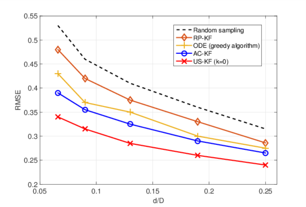
AC-KF and US-KF were run first, with thresholds tuned such that a constant number of approximately observations were selected per time slot; RP-KF and the greedy algorithm were then set to obtain measurements per time slot. As a performance benchmark for the three algorithms, KF was also run with randomly sampled observations per time step.
The average RMSE of the five methods as a function of is plotted in Fig. 3. These plots confirm that the proposed data-agnostic RP-KF is useful for increasing the accuracy (compared to plain random sampling) when estimating dynamic processes. With regards to the more elaborate algorithms, AC-KF has comparable performance with the KF using greedy OED measurement selection, while being orders of magnitude faster in terms of runtime. Last but not least, the US-KF with outperforms the other methods while maintaining complexity, even when the observation noise is correlated. Finally, the experiment was re-run with and for varying , with the runtime of the algorithms listed in Table II. The greedy ODE algorithm is excluded from this experiment since it is an offline benchmark with runtime larger than that of the full-data KF. In comparison to random sampling, the proposed methods carry a certain computational overhead which becomes less significant as (or ) increases. More importantly, the proposed algorithms enjoy a significantly lower runtime than the full-data KF.
Additional experiments were performed to assess sensitivity of the US-KF to the choice of parameter . Recall that determines the accuracy of the approximation of (cf. (22)-(23)), and therefore how accurately the update selection rule in (V) is implemented; at the same time, the computational complexity of implementing (V) increases with at a rate of . Interestingly, experiments indicate that can be sufficient in practice, while sensitivity to only manifests itself for relatively small values of the compression ratio . As seen in Fig. 4, RMSE of US-KF with is almost as low as the one achieved with , while setting still yields reliable estimates, with the gap becoming smaller as increases. Recall that using leads to the simple rule in (24), and bears the additional advantage that no eigenpairs of need be tracked.
| Random sampling | sec | sec | sec |
| RP-KF | sec | sec | sec |
| AC-KF | sec | sec | sec |
| US-KF | sec | sec | sec |
| Full-data KF | sec | sec | sec |
VII-B Bud-KS
In the last experiment, the extent to which backward smoothing iterations can improve reduced-observation filtering was examined. The AC-KF algorithm was first run with ranging from up to ; Bud-KF was then run with in order to smooth all filtered estimates. Figure 5 depicts the average RMSE of the AC-KF with and without smoothing. Evidently, smoothing can significantly reduce RMSE over the entire range of dimensionality reduction, while its effect becomes more prominent as decreases. Upon examining Fig. 5, the AC-KF using of the data followed by Bud-KS, attains the same RMSE as the AC-KF using of the data; a surprising five-fold decrease. Thus, at the cost of introducing non-causality (or delay if a fixed-lag KS is used), smoothing offers room for significant decrease in the data requirements and complexity of tracking.


VIII Application to monitoring dynamic graphs
Dynamically evolving graphs offer a promising application domain for our proposed algorithms. In this context, measurements are obtained from a graph of known and constant topology in order to infer a set of hidden time-varying properties. Specifically, traffic matrix estimation and link cost estimation are two tasks that involve tracking of large-scale dynamical processes from linearly obtained observations. To demonstrate the applicability of US-KF in reducing the complexity of such tasks, a Kronecker graph with vertices was generated. The adjacency matrix of a Kronecker graph can be generated recursively as , and is completely determined by the initiator graph . As shown in [29], Kronecker graphs exhibit many real-word graph properties such as power-law degree distributions, and are thus highly recommended for simulating algorithms. For our experiments, a Kronecker graph was generated with initiator
until nodes become available. Nodes adjacent to all other nodes were removed in order to decrease the connectivity of the graph to more realistic levels. The resulting adjacency matrix is depicted in Fig. 6.

VIII-A Traffic matrix estimation
Consider the task of measuring the traffic volume at the links of a network, in order to estimate the volume of origin-to-destination (OD) flows, a very important task in many networks ranging from the Internet to transportation. Since OD flows are defined by a set of origins and a set of destinations , they can be represented as the entries an traffic matrix . Similar to [30], [31] and [32], the following linear state-transition and observation models is considered
| (38) | ||||
| (39) |
where is the vectorized traffic matrix at time slot that is assumed to evolve according to a random walk with driving Gaussian noise with known covariance matrix such that ; contains the link measurements at time slot ; and, is the observation noise with . The choice of a non-diagonal was made to reflect the fact that flows tend to be highly correlated (see e.g. [2]). For this experiment, we set , , and generated the initial state as In this model, the role of the measurement matrix is played by the routing matrix , each column of which corresponds to an OD flow with entries taking the value , if the corresponding links are part of the flow. Simply put, each column of describes the path that the corresponding OD flow takes through the graph. For this experiment, OD paths were chosen to be the shortest possible using Dijkstra’s algorithm. To make this experiment even more challenging, flows with paths that consist of a single link were not considered; flows with no sampled links and irrelevant links were also removed from the model. Overall, edges were sampled in order to track OD flows.
Plotted in Fig. 7 is the MSE () of the estimated traffic matrix across time, for the proposed US-KF (Alg.4), and the KF with random sampling. The algorithms were run for time slots and the results were averaged across runs. Both algorithms were tuned to utilize of edge measurements per time slot, and require approximately the same runtime. As seen in the plot, the estimates of the proposed US-KF converge faster than those of the sub-sampled KF, and keep a closer track of the true traffic matrix . It should be noted that, due to the large state dimension, other methods such as the RP-KF or greedy OED become impractical.


VIII-B Estimation of link costs from path-cost measurements
Consider now that every edge of the graph is associated with a cost , and that the concatenation of all such costs forms the link cost vector . A common task associated with networks is inference of by measuring path costs , where is the total cost of a flow between nodes and (see e.g., [2, Chap. 9.4.1]). Since is the aggregation of all costs of the edges that the corresponding path crosses, it can be expressed as the inner product between and the corresponding row of the routing matrix. Consequently, path costs and link costs are linked through the linear observation model , where is the vector with all the available path cost measurements. Considering dynamic graphs where the link costs and path costs evolve across time slots , leads to the familiar linear state-transition and state-observation models
| (40) | ||||
| (41) |
where , , and the initial state is . For this experiment, we used the same graph and routing matrix as in the traffic estimation experiment, and generated and according to (40) and (41) correspondingly, with , , and .
Plotted in Fig. 8 is the MSE () of the estimated link costs across time, for the proposed US-KF (Alg.4) and the KF with random sampling, for time slots and averaged across runs. Both algorithms were tuned to utilize of path cost measurements per time slot, and require approximately the same runtime. As seen in the plot, the proposed US-KF successfully tracks the slowly evolving link costs by judiciously selecting and using a small fraction of the available path cost observations. Furthermore, it can be observed that if the same fraction () of measurements is selected at random, then the KF fails to track the link costs, with its estimate diverging from the true value as time progresses. The divergence of the KF with random sampling is consistent with the results in [33], where it is shown that there exists a cut-off value for the data rate, below which the error covariance may become unbounded. Interestingly, the proposed reduced-complexity US-KF appears to be much more robust to divergence; as discussed in the following remark.
Remark 4: While KF based on random sampling (as well RP-KF) diverges when the compression ratio becomes smaller than a certain threshold, this is not the case for the advocated censoring-based alternatives (AC-KF and US-KF) since diverging estimates prohibit censoring. This becomes evident upon realizing that a diverging estimate (i.e., ) would imply infinitely large innovations that cannot be smaller than finite thresholds such as the ones used in censoring rules (8) and (V). This in turn implies that if AC-KF and US-KF were divergent, they would become equivalent to the full data KF. In a nutshell, if the ordinary KF is not divergent, the same holds for the proposed AC-KF and US-KF, since the latter will always obtain sets of observations that guarantee a bounded tracking error.
IX Concluding Remarks
We introduced random projections and censoring as dimensionality reduction and measurement selection methods for tracking dynamical processes with generally time-varying parameters. The proposed methods are simple routines that can be used as dimensionality reduction modules coupled with an ordinary KF. Furthermore, we introduced a reduced-complexity KF that processes measurements sequentially and performs updates that are deemed informative based on the information gain of corresponding measurements. Performance was not analytically performed, but simulations provide surprisingly strong evidence that the proposed methods perform close to the greedy measurement selection method in terms of estimation error. Furthermore, censoring-based measurement selection enjoys much lower computational complexity than greedy OED. To demonstrate applicability of the proposed update selection approach on real-world problems, we examined the network-related applications of traffic matrix estimation and network flow estimation.
Proof:
Follows readily from Theorem 2 in [34].
∎
Proof:
From the assumption of large and uncorrelated noise , the inverse reduced innovation covariance matrix can be approximated as
and hence the correction update as
| (42) |
where . Furthermore, for the censoring rule in (9) simplifies to , where . If is unbiased, then it readily follows that is also unbiased, and (42) yields
| (43) |
Since
| (44) |
where , it follows from (44) and (43) that , and the AC-KF is unbiased.
∎
Proof:
For observations generated according to the linear Gaussian model, and since is the MMSE estimator of given and , it follows that the posterior of is also Gaussian with . Similarly, one can obtain . Using the closed-form identity for the KL divergence between two multivariate normal pdfs, we arrive at
| (45) |
where denotes the trace of matrix and its determinant.
Upon observing that for the RLS-like iteration in (12) the inverse of the covariance matrix is updated as
| (47) |
the fourth summand in (45) can be expressed as
| (48) |
where in the first equality we used the fact that , and in the fourth one we applied the matrix determinant lemma for rank-one updates.
Finally, since , the second summand in (45) becomes
| (49) |
Proof:
By the definition of in (16) and expressing using arguments similar to (46) and (48), it follows that
| (50) |
Utilizing (47) and that yields
and since and the proposition holds. ∎
Proof:
Recalling that and , (25) yields
| (51) |
With denoting the error vector, (51) can be expressed as
| (52) |
The outer product of both sides in (52) yields
| (53) |
Since is unbiased, it follows that is unbiased too, and therefore the MSE equals the trace of the covariance matrix. Since the expected value of the second summand in (53) is zero, the trace of the expectation in (53) yields
| (54) |
where is the covariance matrix after the first-order update in (25). Given that , and upon observing that and , the proof is complete after using (54). ∎
References
- [1] P. Louka, G. Galanis, N. Siebert, G. Kariniotakis, P. Katsafados, I. Pytharoulis, and G. Kallos, “Improvements in wind speed forecasts for wind power prediction purposes using Kalman filtering,” J. of Wind Engin. and Indust. Aero., vol. 96, no. 12, pp. 2348–2362, Nov. 2008.
- [2] E. D. Kolaczyk, Statistical Analysis of Network Data. Springer, 2009.
- [3] H. Zhu, I. D. Schizas, and G. B. Giannakis, “Power-efficient dimensionality reduction for distributed channel-aware Kalman tracking using WSNs,” IEEE Trans. Sig. Proc., vol. 57, pp. 3193–3207, Aug. 2009.
- [4] H. Ma, Y.-H. Yang, Y. Chen, K. R. Liu, and Q. Wang, “Distributed state estimation with dimension reduction preprocessing,” IEEE Trans. Sig. Proc., vol. 62, no. 12, pp. 3098–3110, Dec. 2014.
- [5] M. P. Vitus, W. Zhang, A. Abate, J. Hu, and C. J. Tomlin, “On efficient sensor scheduling for linear dynamical systems,” Automatica, vol. 48, no. 10, pp. 2482–2493, 2012.
- [6] H. Wang, K. Yao, G. Pottie, and D. Estrin, “Entropy-based sensor selection heuristic for target localization,” in Proc. of Intl. Symposium on Information Processing in Sensor Networks, Berkeley, California, 2004, pp. 36–45.
- [7] E. Ertin, J. W. Fisher, and L. C. Potter, “Maximum mutual information principle for dynamic sensor query problems,” in Information Processing in Sensor Networks. Springer, 2003, pp. 405–416.
- [8] L. Zuo, R. Niu, and P. K. Varshney, “Posterior CRLB based sensor selection for target tracking in sensor networks,” in Proc. of Intl. Conf. on Acoust., Speech and Signal Proc., vol. 2, Honolulu, Hawaii, 2007, pp. II–1041.
- [9] S. Joshi and S. Boyd, “Sensor selection via convex optimization,” IEEE Trans. Sig. Proc., vol. 57, no. 2, pp. 451–462, 2009.
- [10] F. Altenbach, S. Corroy, G. Bocherer, and R. Mathar, “Strategies for distributed sensor selection using convex optimization,” in Proc. of GLOBECOM Conf., Anaheim, CA, 2012, pp. 2367–2372.
- [11] M. Shamaiah, S. Banerjee, and H. Vikalo, “Greedy sensor selection: Leveraging submodularity,” in Proc. of 49th Conf. on Decision and Control, Atlanta, Dec. 2010, pp. 2572–2577.
- [12] N. Moshtagh, L. Chen, and R. Mehra, “Optimal measurement selection for any-time Kalman filtering with processing constraints,” in Proceedings of the 48th Conf. on Decision and Control, Shanghai, China, 2009, pp. 5074–5079.
- [13] E. Msechu and G. B. Giannakis, “Sensor–centric data reduction for estimation with WSNs via censoring and quantization,” IEEE Trans. Sig. Proc., vol. 60, no. 1, pp. 400–414, Jan. 2012.
- [14] K. You, L. Xie, and S. Song, “Asymptotically optimal parameter estimation with scheduled measurements,” IEEE Trans. Sig. Proc., vol. 61, no. 14, pp. 3521–3531, July 2013.
- [15] Q. Liu, Z. Wang, X. He, and D. Zhou, “A survey of event-based strategies on control and estimation,” Systems Science & Control Engineering Open Access Journal, vol. 2, no. 1, pp. 90–97, 2014.
- [16] G. Battistelli, A. Benavoli, and L. Chisci, “Data-driven strategies for selective data transmission in sensor networks,” in Proc. of 51st Conf. on Decision and Control, Grand Wailea, Maui, 2012, pp. 800–805.
- [17] Y. Zheng, R. Niu, and P. K. Varshney, “Sequential Bayesian estimation with censored data for multi-sensor systems,” IEEE Trans. Sig. Proc., vol. 62, no. 10, pp. 2626–2641, Oct. 2014.
- [18] G. Wang, J. Chen, J. Sun, and Y. Cai, “Power scheduling of Kalman filtering in wireless sensor networks with data packet drops,” arXiv preprint arXiv:1312.3269v2, 2013.
- [19] Y. Bar-Shalom, X. R. Li, and T. Kirubarajan, Estimation with Applications to Tracking and Navigation: Theory, Algorithms and Software. John Wiley & Sons, 2004.
- [20] M. Mahoney, “Randomized algorithms for matrices and data,” Found. Trends. in Mach. Learn., vol. 3, no. 2, pp. 123–224, 2011.
- [21] P. Drineas, M. W. Mahoney, and S. Muthukrishnan, “Sampling algorithms for l 2 regression and applications,” in Proc. of the 17-th SIAM-ACM Symp. on Discrete Alg., Miami, Florida, 2006, pp. 1127–1136.
- [22] D. P. Woodruff, “Sketching as a tool for numerical linear algebra,” Found. and Trends in Theor. Computer Science, vol. 10, pp. 1–157, 2014.
- [23] Y. Wang, V. Krishnaswami, and G. Rizzoni, “Event-based estimation of indicated torque for IC engines using sliding-mode observers,” Control Engineering Practice, vol. 5, no. 8, pp. 1123–1129, 1997.
- [24] D. Berberidis, V. Kekatos, and G. B. Giannakis, “Online censoring for large-scale regressions with application to streaming big data,” IEEE Trans. Sig. Proc., vol. 64, no. 15, pp. 3854–3867, Aug. 2016.
- [25] S. Kullback and R. A. Leibler, “On information and sufficiency,” The annals of mathematical statistics, vol. 22, no. 1, pp. 79–86, 1951.
- [26] K.-B. Yu, “Recursive updating the eigenvalue decomposition of a covariance matrix,” IEEE Trans. Sig. Proc., vol. 39, no. 5, pp. 1136–1145, 1991.
- [27] M. Gu and S. C. Eisenstat, “A stable and efficient algorithm for the rank-one modification of the symmetric eigenproblem,” SIAM J. on Matrix Anal. and Appl., vol. 15, no. 4, pp. 1266–1276, 1994.
- [28] H. E. Rauch, C. Striebel, and F. Tung, “Maximum likelihood estimates of linear dynamic systems,” AIAA Journal, vol. 3, no. 8, pp. 1445–1450, 1965.
- [29] J. Leskovec, D. Chakrabarti, J. Kleinberg, C. Faloutsos, and Z. Ghahramani, “Kronecker graphs: An approach to modeling networks,” J. Machine Learning Res., vol. 11, pp. 985–1042, 2010.
- [30] K. Rajawat, E. Dall’Anese, and G. B. Giannakis, “Dynamic network delay cartography,” IEEE Trans. Info. Theory, vol. 60, no. 5, pp. 2910–2920, May 2014.
- [31] A. Soule, K. Salamatian, A. Nucci, and N. Taft, “Traffic matrix tracking using Kalman filters,” SIGMETRICS Perform. Eval. Rev., vol. 33, no. 3, pp. 24–31, Dec 2005.
- [32] P. Casas, S. Vaton, L. Fillatre, and L. Chonavel, “Efficient methods for traffic matrix modeling and on-line estimation in large-scale IP networks,” in Proceedings of Intl. Teletraffic Congress, Paris, France, Sept 2009, pp. 1–8.
- [33] B. Sinopoli, L. Schenato, M. Franceschetti, K. Poolla, M. I. Jordan, and S. S. Sastry, “Kalman filtering with intermittent observations,” IEEE Trans. Auto. Cont., vol. 49, no. 9, pp. 1453–1464, 2004.
- [34] P. Drineas, M. W. Mahoney, S. Muthukrishnan, and T. Sarlós, “Faster least squares approximation,” Numerische Mathematik, vol. 117, no. 2, pp. 219–249, 2011.