Resonant inelastic scattering spectra at the Ir $L$-edge in Na₂IrO₃

Neglecting the crystal distortion, we assume each Ir ion in Na₂IrO₃ resides around the center of oxygen octahedra. The energy level of the $e_{g}$ orbitals of Ir atom is about 2-3 eV higher than that of the $t_{2g}$ orbitals due to the crystal electric field of IrO₆. Therefore, taking account of only $t_{2g}$ orbitals, we employ a multi-orbital tight-binding model on a honeycomb lattice, which is defined by

with

where the annihilation ($d_{in\sigma}$) and creation ($d_{in\sigma}^{\dagger}$) operators are for the $5d$ electron with orbital $n$ ($=yz,zx,xy$) and spin $\sigma$ at the Ir site $i$, and $n_{in\sigma}\equiv d_{in\sigma}^{\dagger}d_{in\sigma}$.

The $H_{\rm SO}$ stands for the SOI of $5d$ electrons with ${\bf L}$ and ${\bf S}$ denoting the orbital and spin angular momentum operators, respectively. The $H_{\rm I}$ represents the Coulomb interaction among the $t_{2g}$ electrons, satisfying $U=U^{\prime}+2J$ [33]. We use the values $\zeta_{\rm SO}=0.45$ eV, $U=1.4$ eV, and $J/U=0.15$ in the following calculation. Similar values of the parameters have been utilized for Ir atom in Sr₂IrO₄ [32].

The $H_{\rm kin}$ stands for the kinetic energy of $5d$ electrons with the hopping matrix $\hat{T}_{i,i^{\prime}}$ between the sites $i$ and $i^{\prime}$. The summation $\langle i,i^{\prime}\rangle$ is restricted within the nearest neighbor Ir ions. There exist two kinds of transfer mechanisms between the Ir $5d$ orbitals. The first one is a direct transfer between the Ir $5d$ orbitals, which may be described by means of the Slater-Koster parameters, $V_{dd\sigma}$, $V_{dd\pi}$ ($=-2V_{dd\sigma}/3$), and $V_{dd\delta}$ ($=V_{dd\sigma}/6$)[34]. We may evaluate $V_{dd\sigma}=-0.511$ eV by applying Harrison’s procedure[35]. The second one is an indirect transfer via oxygen $2p$-orbitals. Since the energy required for transferring the electron from oxygen $2p$ levels to Ir $5d$ levels is rather large, the effective transfer between $5d$ orbitals may be estimated by the second-order perturbation. Hence the hopping matrix $\hat{T}_{i,i^{\prime}}^{(pd)}$ may be expressed in a matrix form with the bases $n=yz$, $zx$, $xy$ in order:

where $\langle i,i^{\prime}\rangle$ belongs to bonds 1, 2, and 3, respectively, with the bonds defined in figure 1 (a). The $t_{p}$ may be as large as $\sim 0.25$ eV, which value is similar to the one used in the study of Sr₂IrO₄. The opposite sign had been assigned to $t_{p}$ in our previous paper [29].

We carry out the HFA by following the procedure given in [29]. In that process, we rewrite the Hamiltonian in terms of the Fourier transformed operator with the wave vector ${\bf k}$ within the first magnetic Brillouin zone (MBZ) shown in figure 1(b):

Here, $\lambda$ specifies one of the four sublattices A, B, C, and D, and $N$ is the number of Ir ions. The first MBZ is divided into $40\times 40$ meshes in the numerical calculation. The parameter values are set $\zeta_{\rm SO}=0.45$ eV, $U=1.4$ eV, $J/U=0.15$, $V_{dds}=-0.511$ eV, and $t_{p}=0.25$ eV.

The staggered magnetic moment is known to be directing to the $a$ axis by the experiment [17]. Fixing the staggered moment parallel to the $a$ axis, we carry out the HFA to evaluate the energies of the zigzag, Néel, and stripy ordered states. We find the zigzag ordered state is the most stable. Its energy per Ir ion is 0.09 eV and 0.04 eV smaller than that of the Néel ordered state and that of the stripy ordered state, respectively. The orbital and spin moments align anti-parallel to each other at each site, and their magnitudes are $|\langle L_{a}\rangle|=0.51$ and $|\langle S_{a}\rangle|=0.16$, respectively, where $\langle X\rangle$ represents the ground state average of operator $X$. Hence the total magnetic moment is evaluated as 0.19 $\mu_{B}$, which is comparable to the experimental value of 0.22 $\mu_{B}$.

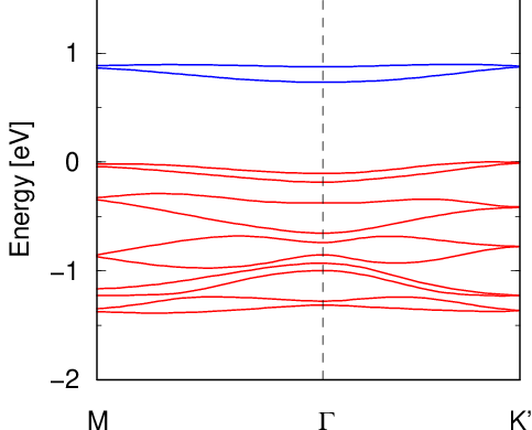
Figure 2 shows the one-electron energy as a function of ${\bf k}$ along symmetry directions in the zigzag ordered state. Each line is doubly degenerate. Hence there exist four states per unit cell in the conduction band. The energy gap is found as large as $\sim 0.8$ eV, and the dependence on ${\bf k}$ is rather weak. The ”$j_{\rm eff}=\frac{1}{2}$” states have the largest weight for the conduction band. The band gap seems overestimated in comparison with the SIC-DFT calculation[28].

In the dipole transition, the $2p$ core-electron is excited to the $5d$ states by absorbing photon at the $L$ edge (and the reverse process). This process may be described by the interaction

where $c_{\alpha}({\bf q})$ is the annihilation operator of photon with momentum ${\bf q}$ and polarization $\alpha$. The $p_{ij_{\rm{c}}m}$ is the annihilation operator of core electron with the angular momentum $j_{\rm{c}}$ ($=\frac{3}{2}$, $\frac{1}{2}$), and magnetic quantum number $m$ at site $i$. The $w(n\sigma;j_{\rm{c}}m;\alpha)$ represents the matrix elements of the $2p\to 5d$ transition, which explicit values for $\alpha=x,y,$ and $z$ are listed in Table I of [32]. In the Fourier transform representation, (7) may be rewritten as

with

where ${\bf k}$ is defined on the first MBZ in the honeycomb lattice. The photon momentum ${\bf q}$ is now regarded as the photon momentum projected onto the two-dimensional $ab$ plane. Here $[{\bf k+q}]$ indicates the vector reduced back to the MBZ by a reciprocal vector ${\bf G}$, that is, ${\bf k+q}=[{\bf k+q}]+{\bf G}$, and ${\bf a}_{\lambda}$ is defined by $(0,0)$, $(0,1)$, $(\sqrt{3}/2,3/2)$, and $(\sqrt{3}/2,-1/2)$ in units of $a$ (the nearest neighbor distance) for $\lambda=$ A, B, C, and D, respectively.

The RIXS spectral intensity may be expressed by the second-order optical process,

where the initial state $|\Phi_{\rm i}\rangle$ may be expressed by $c_{\alpha_{\rm i}}^{\dagger}({\bf q}_{\rm i})|0\rangle|{\rm g}\rangle$ with $|{\rm g}\rangle$ denoting the ground state of the matter with energy $\epsilon_{\rm g}$, and $|0\rangle$ denoting the vacuum state with photon, respectively. The intermediate state $|\Phi_{n}\rangle$ may be expressed by $|0\rangle|n\rangle$ with $|n\rangle$ denoting the intermediate state of the matter with energy $\epsilon_{n}$, and $\Gamma_{\rm c}$ stands for the life-time broadening width of the $2p$-core hole state. The state $|\Phi_{f^{\prime}}\rangle$ may be expressed by $c_{\alpha_{\rm f}}^{\dagger}({\bf q}_{\rm f})|0\rangle|f^{\prime}\rangle$ with $|f^{\prime}\rangle$ denoting the excited state of the matter with energy $\epsilon_{f^{\prime}}$. The incident photon has momentum and energy $q_{\rm i}=({\bf q}_{\rm i},\omega_{\rm i})$ with polarization $\alpha_{\rm i}$, while the scattered photon has momentum and energy $q_{\rm f}=({\bf q}_{\rm f},\omega_{\rm f})$ with polarization $\alpha_{\rm f}$. The momentum and energy transferred to the matter are accordingly given by $q=q_{\rm i}-q_{\rm f}=({\bf q},\omega)$.

Most of RIXS experiments have been carried out in a horizontal scattering geometry with the scattering angle $2\theta$ set to be close to 90^∘. In the following analysis, we tentatively assume that the scattering plane is perpendicular to the plane of honeycomb, and is including the $b$ axis, as illustrated in figure 3. Note that only a few degrees of tilt of the scattering plane could sweep the entire Brillouin zone, since $\omega\sim 11.2$ keV at the Ir $L_{3}$ edge. In the coordinate frame with $a$, $b$, and $c$ axes, the polarization vectors are given by

Note that the $t_{2g}$ states, $yz$, $zx$, and $xy$, as well as the polarizations in $w(n\sigma;j_{\rm c}m;\alpha)$ are defined in the cubic coordinate frame.

Since the value of $\Gamma_{\rm c}$ ($\sim 2.5$ eV) is much larger than a variation of $\epsilon_{n}$ with $n$, the energy denominator of (10) could be factored out in a reasonable accuracy. This procedure is called as the FCA, and (10) may be rewritten as

with

where $E_{0}$ stands for a typical energy of the conduction band. Using the Fourier transform representation, (16) is rewritten as,

where

with $\xi=(\lambda,n,\sigma)$ and $\xi^{\prime}=(\lambda^{\prime},n^{\prime},\sigma^{\prime})$. The summations for $\alpha$ and $\alpha^{\prime}$ run over $x,y,$ and $z$. The $\hat{M}(\mbox{\boldmath{$\alpha$}}_{\rm i},\mbox{\boldmath{$\alpha$}}_{\rm f};j_{\rm c})$ is regarded as a vector with 576 dimensions. The $\hat{Y}^{+-}(q)$ represents the generalized density-density correlation function defined by

with

Thereby $\hat{Y}^{+-}(q)$ is a matrix of $576\times 576$ dimensions. Since an extra phase factor ${\rm e}^{-i{\bf G}\cdot{\bf a}_{\lambda}}$ is contained in (21), the RIXS intensities may become different between the inside and the outside of the first MBZ.

Now that the RIXS spectra are connected with the density-density correlation function, we outline the procedure to calculate it within the RPA. See [29] for details.

Let us introduce the two-particle Green’s function,

where $T$ denoting the time ordering operator and $X(t)\equiv{\rm e}^{iHt}X{\rm e}^{-iHt}$. By taking account of the multiple scattering between particle-hole pair, it is expressed as

where $\hat{\Gamma}$ stands for the antisymmetrized vertex function, which is expressed as

with $g$ defined by the coefficient in the Coulomb interaction,

Then, $\hat{F}(q)$ in (23) is defined as

where $\hat{G}({\bf k},\omega)$ stands for the single-particle Green’s function:

This may be written within the HFA as

where ${\rm sgn}[A]$ stands for a sign of quantity $A$ and $\delta$ denotes a positive convergent factor. The $E_{\ell}({\bf k})$ and $[\hat{U}({\bf k})]_{\xi,\ell}$ stand for the $\ell$-th energy eigenvalue measured from the chemical potential and the corresponding wave function, respectively. By inserting (28) into (26), we have

Once we obtain the two-particle Green’s function $\hat{Y}^{{\rm T}}(q)$, we can evaluate the density-density correlation function $\hat{Y}^{+-}(q)$ with the help of the fluctuation-dissipation theorem,

Panel (a) in figure 4 shows the calculated bound-state energy $\omega_{B}({\bf q})$ as a function of ${\bf q}$ along the symmetry directions in the low-energy region. We find that four gapped excitation modes reside below 20 meV, which may be identified as magnetic excitations. Such small energy scale is consistent with the energy difference between the zigzag and other magnetic orders discussed in Sec. II.2. The presence of four modes may be consistent with the spin-wave excitations in the localized $j_{\rm eff}=\frac{1}{2}$ spin model in the zigzag ordered state. At the K’ point, four modes become two pairs of degenerate modes. Experimentally, the magnetic excitations have been identified below 6 meV by INS [12] and found extending up to 35 meV by RIXS [11]. It suggests there exist at least two magnetic excitation modes, which is consistent with our results. Finally, the excitation energy becomes smaller with ${\bf q}$ away from the $\Gamma$ point in qualitative agreement with the RIXS experiment[11].

Panels (b) and (c) in figure 4 show the RIXS spectra as a function of $\omega$ for ${\bf q}$ from the $\Gamma$ to the M points and the $\Gamma$ to K’ points, respectively. The $\delta$-function peaks are convoluted with the Lorentzian function with the half width of half maximum 1 meV. Among four modes, two upper-energy modes have intensities much larger than two lower-energy modes in the present scattering geometry.

Following the same procedure as the magnetic excitations, we find sixteen bound states for $0.4<\omega_{B}({\bf q})<0.8$ eV below the energy continuum of individual electron-hole pair excitations in the density-density correlation function, which may be identified as excitonic excitations. They are composed mainly of a pair of $j_{\rm eff}=\frac{1}{2}$ electron and $j_{\rm eff}=\frac{3}{2}$ hole. The presence of sixteen modes may be consistent with the localized excitations from $j_{\rm eff}=\frac{3}{2}$ to $\frac{1}{2}$ states for four Ir ions in the unit cell of the zigzag ordering state. The continuous spectra are roughly estimated by sorting $E_{\ell}({\bf k+q})-E_{\ell^{\prime}}({\bf k})$ into segments with the width 0.05 eV in (29), resulting in a histogram representation.

Figure 5 shows the calculated RIXS spectra as a function of $\omega$ for ${\bf q}$ from the $\Gamma$ to the K’ points. The spectra are convoluted with the Lorentzian function with the half width of half maximum 0.04 eV. Arrows indicates the lowest boundary of the energy continuum. We have three prominent peaks. In the RIXS experiment, three peaks named A, B, and C have been observed at $\omega\sim 0.42$ eV, $0.72$ eV, and $0.83$ eV, respectively, with little momentum dependence [10]. The structure found in our calculated spectra seems to agree qualitatively with that derived from the calculation on a small cluster [36] and the experimental spectra[10].